A semantic measure of the execution time in ... - Semantic Scholar

A semantic measure of the execution time in Linear Logic Daniel de Carvalho

Michele Pagani

Lorenzo Tortora de Falco

December 31, 2007 Abstract We give a semantic account of the execution time (i.e. the number of cut-elimination steps leading to the normal form) of an untyped M ELL (proof-)net. We first prove that: 1) a net is head-normalizable (i.e. normalizable at depth 0) if and only if its interpretation in the multiset based relational semantics is not empty and 2) a net is normalizable if and only if its exhaustive interpretation (a suitable restriction of its interpretation) is not empty. We then define a size on every experiment of a net, and we precisely relate the number of cut-elimination steps of every stratified reduction sequence to the size of a particular experiment. Finally, we give a semantic measure of execution time: we prove that we can compute the number of cutelimination steps leading to a cut free normal form of the net obtained by connecting two cut free nets by means of a cut link, from the interpretations of the two cut free nets. These results are inspired by similar ones obtained by the first author for the (untyped) lambda-calculus.

1

Introduction

Right from the start, Linear Logic (LL,[Gir87]) appeared as a potential logical tool to study computational complexity. The logical status given by the exponentials (the new connectives of LL) to the operations of erasing and copying (corresponding to the structural rules of intuitionistic logic and of classical logic) shed a new light on the duplication process responsible of the “explosion” of the size (and time) during the cut-elimination procedure. This is witnessed by the contribution given by LL to the wide research area called Implicit Computational Complexity: a true breakthrough with this respect is Girard’s Light Linear Logic (LLL,[Gir98]). A very careful handling of LL’s exponentials allows the author to keep enough control on the duplication process, and to prove that a function f is representable in LLL if and only if f is polytime. More recently, other “light systems” have been introduced by Asperti and Roversi [AR02], Danos and Joinet [DJ03], Lafont [Laf04] and others: several simplifications are proposed and suggest that LLL is only one among the possible solutions (rather a research theme than a logical system). Light systems can be presented as subsystems of LL obtained by restricting the use of the exponentials: some principles (formulas) provable in LL do not hold in light systems. However, a more geometric perspective on light logic is possible. It comes from the introduction of proof-nets, a geometric way of representing computations; actually one of the most important consequences of the logical status given by LL to the structural rules. Light proofs have been presented in [Gir98] as proof-nets. This viewpoint was stressed in [DJ03]: the authors give a geometric characterization of ELL proof-nets, that is proof-nets belonging to a subsystem of LLL where the functions computable in elementary time (and only those functions) are representable. The system of LL proof-nets is not modified and a global condition on the graph representation of proofs allows to isolate the ones belonging to ELL. A similar work for LLL has been done in [Maz06]. We believe that it is not by eliminating objects with a “bad” computational behaviour that we learn something on the very nature of bounded time complexity, but rather by comparing different computational behaviours, and by finding abstract ways to distinguish the ones from the others. This is, in our opinion, the interest of works like [DJ03] and [Maz06]. Following this kind of idea, in [LTdF06] a new approach to one of the main questions arisen from [Gir98] (maybe the main one), the quest of a denotational semantics suitable for light systems (a semantics of proofs in logical terms, or more generally a model), is proposed. Instead of modifying (like in the previous proposals: [MO00, Bai04]) the structures (games, coherent spaces) associated with logical formulas1 so that the principles valid in LL but not in the chosen light system do not hold in the semantics, [LTdF06] deals with a property of the elements of the structures (the interpretations of proofs) characterizing those elements which can interpret proofs with bounded complexity. In [LTdF06], it is proved in particular that an LL proof-net is an ELL proof-net iff its interpretation is “obsessional”. That is, the semantic property “being obsessional” characterizes, among the interpretations of all LL proof-nets, those ones which are interpretations of ELL proof-nets. 1 The basic pattern of denotational semantics is to associate with every formula some structure and with every proof of the formula an element of the structure called the interpretation of the proof.

1

If one seeks a semantic/mathematical point of view on bounded time complexity, one of the limits of [LTdF06] is the choice of the logical systems to represent elementary/polynomial time. The previoulsy mentioned result, for example, gives a characterization of ELL proof-nets; but there exist LL proof-nets which are not ELL proof-nets and can nevertheless be “executed” in elementary time (i.e., roughly speaking, adding them to ELL does not prevent the cut-elimination procedure from being elementary). This is often the case for systems (of λ-terms, proofs, etc...) characterizing a complexity class: not all the objects excluded have a “bad” complexity behaviour. A different approach to the semantics of bounded time complexity is possible: the basic idea is to measure (by semantic means) the execution of any program, regardless to its computational complexity, in the spirit of comparing different computational behaviours to learn (afterwards) something on the very nature of bounded time complexity. Following this approach, in [dC07, dC] one of the authors of the present paper could compute the execution time of an untyped λ-term via its interpretation in the co-Kleisli category of the comonad associated with the finite multisets functor on the category Rel. The interpretation of a λ-term in this model is the same as the interpretation of the net translating the λ-term in the multiset based relational model of linear logic. The execution time is measured here in terms of elementary steps of the so-called Krivine’s machine. Also, [dC07, dC] give a precise relation between an intersection types system introduced by [CDCV80] and experiments in the multiset based relational model. Experiments are a tool introduced by Girard in [Gir87] allowing to compute the interpretation of proof-nets directly (without reference to sequent calculus) and pointwise. An experiment corresponds to a type derivation and the result of an experiment corresponds to a type. The intersection types system considered in [dC07, dC] lacks idempotency and this fact was crucial in this work. In our work, this corresponds to the fact that we use multisets for intrepreting exponentials and not sets as in the set based coherent semantics. The use of multisets is essential in our work too. In the present paper, we apply this approach to Multiplicative and Exponential Linear Logic (MELL), and we show how it is possible to compute the number of steps of cut-elimination by semantic means (notice that our measure being the number of cut-elimination steps, here is a first difference with [dC07, dC] where Krivine’s machine was used to measure execution time). Let us be more precise: if π2 is a proof-net obtained by applying some steps of cut-elimination to π1 , the main property of any model is that the interpretation Jπ1 K of π1 is the same as the interpretation Jπ2 K of π2 , so that from Jπ1 K it is clearly impossible to determine the number of steps leading from π1 to π2 . Nevertheless, if π1 and π2 are two cut free proof-nets connected by means of a cut link, we can wonder: • is it the case that the thus obtained net can be reduced to a cut free one? • if the answer to the previous question is positive, what is the number of cut reduction steps leading from the net with cut to a cut free one? The main point of the paper is to show that it is possible to answer both these questions by only referring to Jπ1 K and Jπ2 K. Notice that the first question makes sense only in an untyped framework (in the typed case, we know that cutelimination is strongly normalizing, see [Gir87] and [Dan90]), and indeed section 2 is devoted to define an untyped version of Girard’s proof-nets, based on previous works (mainly [Dan90] and [Reg92], [LTdF06], [PTdF07]). Following [PTdF07], we first define pure structures (corresponding in the typed case to proof structures, graphs which are not necessarily logically correct proofs) and we define cut-elimination for pure structures. More generally, in the whole paper we use correctness (in our framework Definition 8) only when it is needed (and it is rarely the case!): this allows to precisely determine where and how correctness is used to prove results. The cut-elimination procedure we define is similar to λ-calculus β-reduction, in the sense that the exponential step (the step (!/?) of Definition 6) is much more similar to a step of β-reduction than it usually is. This is essential to prove our results (see Remark 10). We consider in the paper two reduction strategies: head reduction and stratified reduction. The first one consists in reducing the cuts at depth 0 and stop. The second one consists in reducing a cut only when there exists no cut with (strictly) smaller depth. These reduction strategies extend the head linear reduction of λ-calculus implemented by Krivine’s machine (and considered in [MP94] in the framework of pure proof-nets). In section 3, we introduce the model allowing to measure the number of cut-elimination steps. Experiments are a central tool in our approach. An experiment lives in between syntax and semantics: it is defined on a pure structure (it depends on it), but its “result” (that is the labels it associates with the conclusions of the pure structure) is a point of the interpretation of the pure structure. Taking as starting point the usual multiset based relational model and the usual notion of experiment for this model, we are faced to a problem: an important lemma (Lemma 23) requires the interpretations of ⊗ (resp. 1, !) and (resp. ⊥, ?) to be different (see also the introduction of section 3), because we don’t consider only intuitionistic nets as in [dC05]. We thus define experiments like in [LTdF06], where the distinction between dual constructions was also necessary. This choice of experiments has a categorical counterpart, which is discussed in section 3. What we need is an object of the category Rel, allowing to shift from a typed to an untyped model in such a way that dual logical contructions

2

are interpreted differently in the model. We outline in subsection 3.1 a categorical interpretation of untyped MELL, and we define such an object (so as the required morphisms) in subsection 3.2. We conclude the section with the definition of experiment (Definition 11 of subsection 3.3). In section 4, we give a clear account of the importance of the notion of experiment for our purposes, by proving the Key-lemma (Lemma 20): experiments can be used as counters for cut-elimination steps. Indeed, the Key-lemma shows that every cut-elimination step makes the (suitable notion of) size of an experiment decrease exactly by 2. All our results essentially rely on this lemma. The first step we then accomplish is to precisely relate head and stratified reductions to experiments. Proposition 24 (resp. Proposition 34) proves that a net is head-reducible (resp. stratified-reducible) to an head-cut free net (resp. a cut free net) π ′ if, and only if, it has at least one experiment (resp. one exhaustive experiment, see Definition 30). These results are the analogue of classical results for λ-terms: a λ-term is head-normalizable (resp. weak normalizable) if, and only if, it is typeable in the appropriate intersection types system. Then we give a quantitative insigth of this correspondence reduction/experiment: Theorem 27 (resp. Theorem 38) recovers the number of head (resp. stratified) reduction steps from π to a head-cut free (resp. cut free) π ′ from the notion of size of an experiment (resp. of an exhaustive experiment). These results are first proved for the head reduction (Subsection 4.1) and then extended to the stratified reduction (Subsection 4.2). Finally, section 5 allows to shift from experiments to their results, thus giving the required relation between semantics and execution time. We prove that we can answer both the initially stated questions by only referring to Jπ1 K and Jπ2 K. This shows that a (rather precise) notion of time is still present in the denotational interpretation of a net. Let us conclude with a little remark. In [TdF03], the question of injectivity for the relational and coherent semantics of LL is adressed: is it the case that for π and π ′ cut free, from JπK = Jπ ′ K one can deduce π = π ′ ? It is conjectured that relational semantics is injective for MELL, and there is still no answer to this question. Given π1 and π2 , we don’t know how to compute the normal form of the net obtained by connecting π1 and π2 by means of a cut link from Jπ1 K and Jπ2 K. However, the present paper shows that from Jπ1 K and Jπ2 K we can at least compute the number of cut-elimination steps leading to a normal form.

2

Proof-nets

After their introduction by Girard in [Gir87], proof-nets have been extensivley studied and used as a prooftheoretical tool for several purposes. All this work led to many improvements of the original notion introduced by Girard. We use here an untyped version of Girard’s proof-nets. Danos and Regnier ([Dan90] and [Reg92]) introduced and studied “pure proof-nets” that is the exact notion of proof-net corresponding to the (untyped) λ-calculus. There has been no real need for a different notion of untyped proof-net until Girard’s work on Light Linear Logic ([Gir98]): using the fact that the complexity of the cut-elimination procedure does not depend on types (a key property of light systems) Terui ([Ter02]) introduces a “light” (untyped) λ-calculus enjoying strong normalization in polynomial time and encoding all polytime functions. This calculus clearly corresponds to an untyped version of ILAL’s proof-nets (ILAL is an intuitionistic variant of LLL, see [AR02]. See also [BM04] for a similar result). In the same spirit, an untyped notion of proof-net (called net ) is introduced in [LTdF06] in order to encode polytime computations: the novelty here is the shift from the intuitionistic to the classical framework. This immediately yields cuts which cannot be reduced and called clashes (see figure 2). In [PTdF07], in order to prove strong normalization for full second order LL, a further generalization of the notion of [LTdF06] is proposed and studied: the one of pure structure. A pure structure is a net which is not necessarily correct (in the sense of Definition 8). The introduction of proof structures (i.e. graphs which do not always correspond to logically correct proofs) dates back to [Gir87], but it took much time to really start exploiting the presence of such objects (like for example in ludics [Gir99], [Gir01]). Recent works (in particular [PTdF07]) show that we always learn something when we are able to precisely determine where and how correctness is used to prove results. From the perspective of the present work, the notion of pure structure turns out to be the appropriate one: most of our results (but not all of them!) are proved for pure structures. A last comment on the syntax: we choose here a version of pure structures where ?-links have n ≥ 0 premisses (these links are often represented by a tree of contractions and weakenings). We also have a ♭-node which is our way to represent dereliction. These choices are just driven by the attempt to have a(n as much as possible) simple presentation of our results. Notice, however, that the reduction steps (and more precisely the exponential step) have to be defined the way we do it in order for our results to hold (see also Remark 10 and Figure 8). Definition 1 (Flat) A flat is a finite (possibly empty) labelled directed acyclic graph whose nodes (also called links) are defined together with an arity and a coarity, that is a given number of incident edges called the premises 3

ax

cut

⊗

··· ♭

♭ ! ♭

···

⊥

1

♭

♭

?

♭

Figure 1: MELL links of the node and a given number of emergent edges called the conclusions of the node. The valid nodes are in Figure 1. The links are divided into three groups: the ax- and cut-links are called identities; the ⊗-, -, 1- and ⊥-links are called multiplicatives; the !-, ♭- and ?-links are called exponentials. An edge can have or not a ♭ label: an edge with no label (resp. with a ♭ label) is called logical (resp. structural). The ♭-nodes have a logical premise and a structural conclusion, the ?-nodes have k ≥ 0 structural premises and one logical conclusion, the !-nodes have no premise, exactly one logical conclusion, called also main conclusion of the node, and k ≥ 0 structural conclusions, called auxiliary conclusions of the node. Premises and conclusions of identities and multiplicatives are logical edges. We allow edges with a source but no target, they are called conclusions of the flat. The size of a flat α, denoted by s (α), is the number of the logical edges in α. We denote by !(α) the set of !-links of α. Links (resp. edges) will be denoted by middle Latin letters l, m, . . . (resp. initial Latin letters a, b, . . . ); flats will be denoted by initial Greek letters α, β, . . . When drawing a flat we represent edges oriented up-down so that we speak of moving upwardly or downwardly in the graph, and of nodes or edges “above” or “under” a given node/edge. In the sequel we will not write explicitly the orientation of the edges. In order to give more concise pictures, when not misleading, we may represent an arbitrary number of ♭-edges (possibly zero) as a ♭-edge with a diagonal stroke drawn across: ♭ ?

♭

··· ♭

=

as well

?

=

!

♭

! ♭

···

♭

In the same spirit, a ?-link with a diagonal stroke drawn across its conclusion represents an arbitrary number of ?-links (possibly zero): ♭

··· ♭ ?

♭

=

··· ♭ ?

♭ ···

··· ♭ ?

For an example of this notation see Figure 6. Definition 2 (Pure structure) A pure pre-structure (pps for short) π of depth 0 is a flat without !-nodes; in this case, we set flat(π) = π. A pure pre-structure π of depth d + 1 is a flat α, denoted by flat(π), with a function that associates with every !-link o of α with no + 1 conclusions a pps π o of depth at most d, called the box of o, with no structural conclusions corresponding2 to the no auxiliary conclusions of o and exaclty one logical conclusion corresponding to the main conclusion of o. Moreover α has at least one !-link with a box of depth d. For any pure pre-structure π, we define, by induction on depth(π), the size of π, denoted by s(π), as follows : X s(π o ) . s(π) = s(flat(π)) + o∈!(flat(π))

2 We mean here that there exists a bijection from the set of sructural conclusions of the link o to the set of structural conclusions of the pure pre-structure π o .

4

♭ ⊥

⊥ cut

⊥

ax

! cut

cut

!

? cut

Figure 2: example of clashes (the two ps on the left) and of deadlocks (the two ps on the right) The depth of a link l in a pps π is the number of boxes of π containing l. The links of a given flat of a pps all have the same depth, so that the depth of a flat of a given pps is well-defined. A pure structure (ps for short) is a pps with no structural conclusion. Remark 3 Concerning the presence of empty structures, notice that the empty flat does exist and it has no conclusion. Its presence is required by the cut-elimination procedure (Definition 6): the procedure applied (for example) to the ps containing a unique flat consisting of a !-link with only the main conclusion a cut and a ?-link with 0 premises yields the empty graph. On the other hand, notice also that with a !-link o of a pps, it is never possible to associate the empty pps: o has at least one conclusion and this has also to be the case for the pps associated with o. Conventions. Given a link l of a ps π, we will often speak of “the flat of l” always meaning the biggest flat of π containing l. We will sometimes refer to “the maximal flats of a ps”, meaning the flats which are not (strict) subgraphs of other flats of the ps. In general, ps may contain “pathological” cuts (see examples in Figure 2), that is cuts which are not reducible. This is due either to bad “typings” (the cut premises are not dual edges), or to bad “geometric” configurations: in the following definition we call the former clashes and the latter deadlocks. Definition 4 (Clash and deadlock) The two edges premises of a cut-link are dual when : • one is a conclusion of a ⊗-node and the other one is the conclusion of a -node, • one is a conclusion of a 1-node and the other one is the conclusion of a ⊥-node, • one is the main conclusion of a !-node and the other one is the conclusion of a ?-node. A cut-link is: • a clash, when the premises of the cut-node are not dual edges and none of the two is the conclusion of an ax-link; • a deadlock, when the two premises of the cut-link are conclusions of the same ax-link or one of the two is the main conclusion of a !-link o and the other one is the conclusion of a ?-link having among its premises an auxiliary conclusion of o • reducible, otherwise. Remark 5 Notice that with every premise b of a ?-node is associated exactly one ♭-node (which might have depth much greater than the ?-node): we’ll refer to this node as “the ♭-node associated with b”. On the other hand, with every structural conclusion b of a !-link (resp. of a ♭-link) of a ps is associated a unique ?-link: we’ll refer to this node as “the ?-node associated with b”. Definition 6 (Types of cut and cut reduction) Let π be a ps, let t be a reducible cut-link of π, a and b the premises of t, and let α be the (biggest) flat of π containing t at depth 0. We define the flat α′ , obtained by applying some transformations to α (these depend on the type of the cut t). The one step reduct π ′ of π is obtained from π by substituting α′ for α and, in the (!/?)-cases, by slightly modifying the rest of the ps. • (ax): one premise of t, say b is the conclusion of an ax-link (see Figure 3). In this case α′ is obtained by erasing the cut link, its premises a and b and the the axiom, and by connecting the remained conclusion c of the axiom with the node of conclusion a in π; • (⊗/ ): one premise of t is the conclusion of a ⊗-link, the other one is the conclusion of a -link (see Figure 4). In this case α′ is obtained by erasing the -link, the ⊗-link and the cut link t (and its premises) and by putting two new cut links between the two left (resp. right) premises of the -link and of the ⊗-link3 ; • (1/⊥): one premise of t is the conclusion of a 1-link, the other one is the conclusion of a ⊥-link (see Figure 5). In this case α′ is obtained by erasing the three links: 1, ⊥ and the cut (and its premises);4 3 Notice that this means that the premises of the ⊗/ -links are ordered; we shall see in the transformation associated with the (!/?) cut-link that this is not the case of the premises of the ?-links. 4 This case -so as the (!/?) one- might yield an empty graph. 0

5

π

=

ax

t

a

/o /o /o /

c

b

cut

π′

=

c

Figure 3: reduction of a cut of type (ax)

π

f

=

⊗ a

g

h

i

cut t

/o /o /o /

π′

=

f

b

cut

g

h

i cut

Figure 4: reduction of a cut of type (⊗/ )

π

=

⊥

1 a

cut t

/o /o /o /

b

π′

=

Figure 5: reduction of a cut of type (1/⊥) • (!/?)0 : one premise of t is the main conclusion of a !-link and the other one is the conclusion of a ?-link having 0 premises. In this case, the !-link (together with its box) and its conclusion edges are erased. We then erase the ?-link, the cut and its premises. Notice that the ?-links of π associated with the conclusions of the erased !-link have lost some premisses; • (!/?)>0 : one premise of t, say a, is the main conclusion of a !-link and the other one (i.e. b) is the conclusion of a ?-link having b′1 , . . . , b′k as premises, with k ≥ 1 (see Figure 6). Let’s call o the !-link and suppose it has h auxiliary conclusions, let π o be the box5 of o, let w be the ?-link, let vi be the ♭-link associated with b′i , and let βi be the flat of vi . The set {b′1 , . . . , b′k } of w’s premises can be split into two disjoint sets: let C (resp. B) be the set of w’s premises whose associated ♭-link belong (resp. does not belong) to the same flat as w. Consider k copies of o (and of o’s box), call o1 , . . . , ok these !-links and π o1 , . . . , π ok their boxes. Now proceed as follows: • erase t and its premises, w (and its premises), o (and its conclusions and its box) • if b′j ∈ C, then erase the ♭-link vj of α and cut vj ’s premise cj with the main conclusion of the box π oj of oj • if b′j ∈ B, then substitute the flat βj of vj by considering the flat βj− (that is βj where vj and its conclusion have been erased) and by cutting the premise of vj with the main conclusion of π oj . Of course every !-link of π ′ containing this flat has different auxiliary conclusions from the corresponding !-link of π: its auxiliary conclusion corresponding to the conclusion of vj has been substituted by h auxiliary conclusions (the auxiliary conclusions of π oj ) • for every auxiliary conclusion d of o in π, we now have k auxiliary conclusions d1 , . . . , dk of, respectively, π o1 , . . . , π ok . Let l be the ?-node associated with d in π: in π ′ this will be the ?-node associated with d1 , . . . , dk . We denote by t(π) the ps6 obtained applying the transformation previously defined associated with the cut link t. We’ll also refer to t(π) as a one step reduct of π, and to the transformations associated with the different types of cut link as the reduction steps. We write π π ′ , when π ′ is the result of one reduction step. A reduction step is said to be a head reduction step when the reduced cut t has depth 0 in π: we write π h π ′ , when π ′ is the result of one head reduction step. A reduction step π t(π) is said to be a stratified reduction step when for every cut-link (including non-reducible ones) t′ of π we have depth(t) ≤ depth(t′ ): we write π s π ′ when π ′ is the result of one stratified reduction step. 5 Remember 6 The

that π o , so as the pps associated with every !-link, cannot be empty. fact that t(π) is indeed a ps can be easily checked.

6

· ·· ·

·

··

·· c1 β1

v1

ck

··· ♭

♭

βk

vk

♭

♭ !

! ♭

♭

♭

·

··

·

··

π

♭

!

!

=

♭

♭

πo ♭

♭

···

b′k

b′1 !

o a

♭

?

t

b

cut

♭

α

w

! ♭

··

·

♭

! ♭ ♭

♭

?

O O

O

··

·



·

··

·

·· π o1 ♭

π ok

···

c1

ck cut

♭

cut

!

! ♭

♭

♭

·

··

·

··

π′

♭

=

! ♭

♭

!

···

♭ ♭

··· ♭

♭

···

!

··

·

♭

α′

♭ ♭

♭

♭

!

··· ?

Figure 6: reduction of a cut of type (!/?) We denote a reduction sequence R from π to π ′ as the sequence of ps (π1 , . . . , πn ), s.t. R = π π1 ... πn = π ′ . A reduction sequence R is an head reduction (resp. a stratified reduction) when every step of R is an head (resp. a stratified) reduction step. Notice cut reduction is defined on ps and not on pps. This is because we want to leave unchanged the number of conclusions of a structure: this is true only for the logical conclusions, the structural ones may be changed by the (!/?)-steps. In the sequel, however, we need to speak of the cut reduction of a box π o (which is a pps) associated with a !-link o: in that case we mean the cut reduction of the ps obtained by adding to π o the ?-links of π associated with the structural conclusions of π. Notice that the cut reduction cannot be applied to deadlocks nor to clashes, and this means that there are ps (even nets) which are normal w.r.t. cut reduction7 even if they are not cut free (consider for example the ps of Figure 2). 7 I.e.

to which no cut reduction step can be applied.

7

a

ax b

♭ ♭

! u c ♭

v ! h ♭ ♭ ?

♭

♭ ? d o ! f

l

ax i

cut

♭ ♭

♭

g

Figure 7: example of a net which does not normalize. This net reduces to itself by one (!/?) step and one (ax) step Conventions. ∗ , ∗h and

∗ s

Given a binary relarion R, we denote by R∗ its reflexive and transitive closure. So in particular, denote the reflexive and transitive closure of resp. , h and s .

We now give a precise definition of the notions of ancestor and residue of an edge/node: the point is to know whether a given edge/node of t(π) is “created” by the cut reduction procedure or “residue” of some π’s edge/node. Definition 7 (Ancestor, residue) Let π be a ps, t be a cut-link of π and t(π) be the one step reduct of π ← − ← − associated with t. When an edge d (resp. a node l) of t(π) comes from a (unique) edge d (resp. node l ) of ← − ← − ← − π, we say that d (resp. l ) is the ancestor of d (resp. l) in π and that d (resp. l) is a residue of d (resp. ← − l ) in t(π). If this is not the case, then d (resp. l) has no ancestor in π, and we say it is a created edge (resp. node). We indicate, for every type of cut-node t of Definition 6, which edges (resp. links) are created in t(π) (meaning that the other edges (resp. nodes) of t(π) are residues of some π’s node). We use the notations of Definition 6: • (ax): there are no created edges, nor created nodes in t(π). Remark that a, b are erased in t(π), so that we consider c in t(π) the residue of c in π; • (⊗/ ): there are no created edges, while the two new cut-links between the two left (resp. right) premises of the -link and of the ⊗-link are created nodes; • (1/⊥): there are no created edges, nor created nodes in t(π); • (!/?): every auxiliary conclusion added to the !-links containing one π oi is a created edge; every cut link between π oi ’s main conclusion and ci is a created node.8 Definition 8 (Nets) A switching of a flat α is an (undirected) subgraph of α obtained by forgetting the orientation of α’s edges, by deleting one of the two premises of each -node, and for every ?-node l with n ≥ 1 premises, by erasing all but one premises of l. A proof-net, net for short, is a ps π s.t. every switching of every flat of π is an acyclic graph. Remark that the empty ps is a net. Moreover, a net cannot contain deadlocks (while it may contain clashes). Proposition 9 Let π be a net and t be a reducible cut-link of π, then t(π) is a net. Proof. Standard (see [Dan90]).



It is well-known that there are untyped nets non-normalizable, i.e. nets π s.t. any reduction sequence starting from π can be arbitrarily long. The well-known example is the net corresponding to the untyped λ-term (λx.(x)x)λx.(x)x (see [Dan90], [Reg92]). We give in Figure 7 a slight variant (which is not a λ-term), due to Mitsu Okada. Remark 10 The syntax chosen for ps and nets is often called “nouvelle syntaxe”. With respect to our purposes (the semantic measure of cut reduction) this choice is crucial. Indeed, one of the key property we are going to use is the fact that two head (or stratified) reductions of a ps π leading to a cut free ps π0 always have the same length (see Corollary 29). This would be wrong in the “traditional” syntax of nets (the original one of [Gir87], or its untyped version, see [PTdF07]), as the reader can see in the example of Figure 8. 8 Notice that every !-link of π ′ which contains a copy of π o is considered a residue of the corresponding !-link of π, even though it has different auxiliary conclusions.

8

⊥ 1

1

?d

!

1

⊥

! cut

O

!

?d

1

⊥

cut

?d

!

cut u

t

O

?d cut u

}= }= }= = } } =}

O

O 1

/o /o /o /

⊥

⊥

!

?d cut

1

⊥ cut

Figure 8: example of two head reductions with different length in the “traditional syntax”: reducing first the cut t and then the cut u gives the same result as reducing at once u. The reader can check that in our syntax both t(π) and u(π) reduce in exactly one step to the same net.

3

Denotational semantics

We define here the model allowing to measure execution time. It has a categorical presentation, and it is possible to compute the interpretation of nets directly in the model (without using the sequentialization theorem). Our aim is to use the multiset based relational model (in the category Rel), but notice that we want to interpret untyped srtuctures. In Subsection 3.1, we describe the main ingredients necessary to define a model of untyped nets. As it is wellknown, the shift form typed to untyped models essentially relies on the choice of a suitable object in the category used in the typed case. The same applies here, but it turns out that in order for our model to relate precisely interpretations of nets and their execution, duality needs to be “visible” in the semantics. More concretely, we know that in Rel the linear formulas A and A⊥ have the same interpretation. In the absence of types, this means that we do not know whether -say- a couple (x, y) is an element of the interpretation of a formula of the shape A ⊗ B or A B. This information is necessary for our purposes: more precisely we need it to prove Lemma 23 of Subsection 4.1. We show, in Subsection 3.2, how to choose an appropriate object D of Rel. The last Subsection 3.3 is devoted to adapt to our model (i.e. to the choice made in Subsection 3.2) the notion of experiment.

3.1

A categorical framework for interpreting untyped nets

We outline, in this subsection, a categorical interpretation of untyped multiplicative and exponential Linear Logic. We introduce for this purpose a sequent calculus that corresponds to the multiplicative fragment: the sequents are of the shape ⊢ n, where n is a natural integer. ⊢ n exchange with σ ∈ S n ⊢ σ(n) ⊢2

axiom

⊢m+1 ⊢n+1 ⊗ ⊢m+n+1 ⊢1

1

⊢m ⊢n mix ⊢m+n

⊢m+1 ⊢n+1 cut ⊢m+n ⊢n+2 ⊢n+1 ⊢n ⊥ ⊢n+1 ⊢0

daimon

We want to interpret this sequent calculus in a MIX category (see [CS97]

n for the definition of MIX category) in such a way that a sequent ⊢ n is interpreted by a morphism from 1 to i=1 D, where 1 is the unit tensor and D is a particular object of the category. So, we define an object D of the category and 6 morphisms f , g, fD⊗D , fD D , f1 and f⊥ in the category such that : 9

• f is a morphism from D⊥ to D; • g is a morphism from D to D⊥ ; • fX is a morphism from X to D for X ∈ {D ⊗ D, D D, 1, ⊥} that satisfy the following equations : • g ◦ f = idD⊥ ; • fD D ⊥ ◦ g ◦ fD⊗D = g ⊗ g; • fD⊗D ⊥ ◦ g ◦ fD D = g g; • f⊥ ⊥ ◦ g ◦ f1 = id1 • and f1 ⊥ ◦ g ◦ f⊥ = id⊥ . These morphisms are used as follows : • we use f for the interpretation of the axiom rule; • we use g for the interpretation of the cut rule; • we use fX for the interpretation of the X-rule, where X ∈ {⊗, , 1, ⊥}. To accomodate (untyped) exponentials in a categorical structure, we need two more morphisms: • f!D is a morphism from !D to D • and f?D is a morphism from ?D to D such that • f?D ⊥ ◦ g ◦ f!D =!g • and f!D ⊥ ◦ g ◦ f?D =?g.

3.2

Relational semantics for untyped nets

We define, in this subsection, the model where we are going to intepret nets in Subsection 3.3. We start from the well-known category Rel of sets and relations, having in mind the usual multiset based relational model (⊗ and are the cartesian product, 1 and ⊥ are the singleton {∗}, ! and ? are the finite multisets functor). From Subsection 3.1, it is clear that the delicate point is the choice of the object D. It turns out that the more na¨ıve choice of such an object is not suitable for our purposes. Indeed, let A′ be a set that doesn’t contain any couple S ′ nor finite multisets nor ∗. The first idea is to set D = n∈N Dn′ , where Dn′ is defined by induction on n as follows: • D0′ = A′ ∪ {∗} ; ′ • Dn+1 = D0′ ∪ (Dn′ × Dn′ ) ∪ Mf (Dn′ ). We set

and fX

f = g = idD′ = {(x, x) ; x ∈ X} : X → D′

for X ∈ {D′ ⊗ D′ , D′

D′ , 1, ⊥, !D′ , ?D′ } .

The choice of D′ leads to a semantics where nets that have clashes can have a non-empty interpretation. For example, by adding an axiom link to the two clashes of Figure 2, one obtains (following Definition 11 where one substitutes D′ for D) two nets with a non-empty interpretation. This would contradict Lemma 23 of Subsection 4.1, which is essential to prove our main results of Section 5. That’s why we choose another object D (instead of D′ ) of the category of sets and relations, thus obtaining a different model, suitable for our purposes. A key feature of D is that, for every x ∈ D, one has x 6= x⊥ . This will be used to prove Lemma 23 (see also Definition 30 of Subsection 4.2). Let A be a set that doesn’t contain any S couple of the shape (+, x) nor (−, x) and let ψ be an involutive bijection on A without fixpoint. We set D = n∈N Dn , where Dn is defined by induction on n as follows: • D0 = A ⊕ (1 ⊕ ⊥) ; • Dn+1 = D0 ⊕((Dn ⊗ Dn ) ⊕ (Dn Dn )) ⊕ (!Dn ⊕?Dn ), B∪C if B and C are disjoint where B ⊕ C = ({+} × B) ∪ ({−} × C) else. For x ∈ D, depth(x) is the least integer n such that x ∈ Dn . For x ∈ D, we define x⊥ by induction on depth(x): • if x ∈ A, then x⊥ = ψ(x) ; we set (+, ∗)⊥ = (−, ∗) and (−, ∗)⊥ = (+, ∗) ; • we set (+, y)⊥ = (−, y ⊥ ) and (−, y)⊥ = (+, y ⊥ ). We set f = g = {(x⊥ , x) ; x ∈ D} : D → D and

fX = {(x, (+, x)) ; x ∈ X} : X → D fX = {(x, (−, x)) ; x ∈ X} : X → D

10

for X ∈ {D ⊗ D, 1, !D} for X ∈ {D D, ⊥, ?D} .

x

cut x⊥

⊥

1 (+, ∗)

x

y

x

x⊥

x ax

y

⊗

(−, ∗)

(−, x, y)

(+, x, y)

πo ♭ (−, µ1 )

x ♭ ♭ (−, [x])

··· ♭ (−, µn ) ?  P  −, i≤n µi

(−, µi ) ♭ 

−,

P

i≤n

 µi ♭

xi ! [eo1 , . . . , eon ] (+, [x1 , . . . , xn ])

Figure 9: experiments of pure proof-structures Notice that, contrary to the previous case (D′ ), here D ⊗D 6⊆ D (and the same holds for 1, !, , ⊥, ?) and fD⊗D 6= fD D (and the same holds for 1/⊥, !/?). Furthermore, notice that if x ∈ 1, D ⊗ D, !D (resp. x ∈ ⊥, D D, ?D), then (+, x) ∈ D (resp. (−, x) ∈ D). In this categorical structure, we know that we can compute the interpretation of a net directly, that is by experiments and without sequentialization. We do it in the following subsection.

3.3

Experiments

For a pps π with n conclusions c1 , . . . , cn

, we define the interpretation of π according to the sequence

n (cD.1 , . .If. ,ycn=), n denoted by JπK

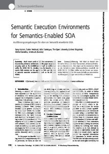
D, that can be seen as a morphism from 1 to c1 ,...,cn , as a subset of i=1 i=1 n (x1 , . . . , xn ) ∈ i=1 D, then yi denote xi . We compute JπKc1 ,...,cn by means of the experiments of π, a notion introduced by Girard in [Gir87] and central in this paper. We define an experiment e of π by induction on the depth of π: remark that the following definition is slightly different from that used in [TdF03], namely e is defined only on the edges of f lat(π). Definition 11 (Experiment) An experiment e of a pure pre-structure π, denoted by e : π, is a function which associates with every !-link o of f lat(π) a multiset [eo1 , . . . , eok ] (k ≥ 0) of experiments of π o , and with every edge a of f lat(π) an element of D, such that if a, b, c are edges of f lat(π) the following conditions hold (see Figure 9): • if a, b are the conclusions (resp. the premises) of an ax-link (resp. cut-link), then e(a) = e(b)⊥ ; • if c is the conclusion of a 1-link (resp. ⊥-link), then e(c) = (+, ∗) (resp. e(c) = (−, ∗)); • if c is the conclusion of a ⊗-link (resp. -link) with premises a, b, then e(c) = (+, e(a), e(b))9 (resp. e(c) = (−, e(a), e(b))); • if c is the conclusion of a ♭-link with premise a, then e(c) = (−, [e(a)]); • if c is the conclusion of a ?-link with premises a1 ,. . . , an , and for every i ≤ n, e(ai ) = (−, µi ), where µi P is a finite multiset of elements of D, then e(c) = −, i≤n µi ; in particular if c has no premises, then e(c) = (−, [ ]); • if c is a conclusion of a !-link o of f lat(π), let π o be the box of o and e(o) = [eo1 , . . . , eon ]. If c is the main conclusion of o, let co be the main conclusion of π o , then e(c) = (+, [eo1 (co ), . . . , eon (co )]), if c is an auxiliary conclusion of o, let co be the auxiliary conclusion of π o associated with c, and for every i ≤ n, let  P o o ei (c ) = (−, µi ), then e(c) = −, i≤n µi . If c1 , . . . , cn are the conclusions of π, then the

result of e according to the sequence (c1 , . . . , cn ), denoted n by |e|c1 ,...,cn , is the element (e(c1 ), . . . , e(cn )) of i=1 D. The interpretation of π according to the sequence (c1 , . . . , cn ) is the set of the results of its experiments: JπKc1 ,...,cn = {|e|c1 ,...,cn ; e : π} . The subscripts

c1 ,...,cn

will be omitted when irrilevant, in which case we simply write JπK or |e|.

In general an experiment e of a ps π is uniquely determined by its values on the axiom conclusions and on the !-links of f lat(π); if moreover π is head-cut free, then any (compatible) choice of values for the axiom conclusions and for the !-links of f lat(π) defines an experiment. In Figure 10 we give some examples of experiments: consider 9 By definition of D, to be precise we should write (+, (e(a), e(b))), but to improve readability we omit here (and in the sequel) some parenthesis and we simply write (+, e(a), e(b)).

11

the net π and the experiment e defined by the topmost net of Figure 10.

If one enumerates π’s conclusions from left to rigth, then one has |e|c1 ,c2 = (−, 2[x] + 2[y]) , −, 2[x⊥ ] + 2[y ⊥ ] . The interpretation of π is: 

 ⊥ (−, [x1 , . . . , x4 ]) , −, [x⊥ ; xi ∈ {(−, ∗) , (+, ∗)} ∪ A, 1 , . . . , x4 ] JπKc1 ,c2 = . for i ≤ 4 The reader can check that every cut reduct of π (for example the nets π2 , π3 , π8 of Figure 10) has the same interpretation as π. Indeed the invariance of the interpretation under cut reduction is a key property, stated by the well-known theorem: Theorem 12 (Soundness) Let π, π ′ be two ps with n conclusions c1 , . . . , cn such that π Jπ ′ Kc1 ,...,cn .

∗

π ′ , then JπKc1 ,...,cn =

Proof. Standard (see [Gir87]): the theorem is also an immediate consequence of our lemma 20.



The empty net has no conclusion and it has exactly one experiment: the unique function with empty domain. It is worth noticing that the interpretation of the empty net is not the empty set: it is the singleton of the empty sequence {( )}. By Theorem 12, this means that every ps reducing to the empty net is interpreted by {( )}. Of course there are ps having an empty interpretation, for example take any ps with an head-clash: no experiment meets the cut condition of Figure 9. More interesting examples of ps having an empty interpretation, are those ps from which starts an infinite head-reduction sequence. The following definition introduces an equivalence relation ∼ on the experiments of a ps π: intuitively the ∼ equivalence classes are made of experiments which associate with a given !-link of π multisets of experiments with same cardinality (but nothing prevents two equivalent experiments from choosing different cardinalities for different !-links). This relation, as well as the notion of substitution defined immediately after, will play a role in Section 5. Definition 13 (Equivalence ∼) For every pps π, we define an equivalence relation ∼ on the set of experiments of π. If π is of depth 0, then, for every e : π, e′ : π, we have e ∼ e′ . Else, for every e : π, e′ : π, we have e ∼ e′ if, and only if, for every !-node o of π, there exists an integer m, there exist e1 : π o , . . . , em : π o , e′1 : π o , . . . , e′m : π o , where π o is the box associated with the node o, such that • we have e(o) = [e1 , . . . , em ] and e′ (o) = [e′1 , . . . , e′m ] ; • and, for every j ∈ {1, . . . , m}, we have ej ∼ e′j . For example, recall the experiment e : π defined on the topmost net of Figure 10: the ∼-equivalence class of e is the set of all experiments of π which takes a multiset of cardinality 4 on the left !-link and a multiset of cardinality 2 on the right !-link. Definition 14 (Substitution) A unary substitution σ is a function from D to D such that • for x ∈ D, σ(x⊥ ) = σ(x)⊥ , • for every y, z ∈ D, we have σ(p, y, z) = (p, σ(y), σ(z)) • and for every x1 , . . . , xm ∈ D, we have σ(p, [x1 , . . . , xm ]) = (p, [σ(x1 ), . . . , σ(xm )]) , where p ∈ {+, −}. We denote by S1 the set of unary substitutions. If ϕ is a function from a subset B of A ∪ {(+, ∗)} to D, then there exists a unique σ ∈ S1 such that for every x ∈ A ∪ {(+, ∗)}, we have  ϕ(x) if x ∈ dom(ϕ) σ(x) = . x if x ∈ / dom(ϕ) ∪ ψ(dom(ϕ))





We denote by ϕ this σ. For every integer n > 1, an n-ary substitution τ is a function from ni=1 D to ni=1 D

n such that there exists σ ∈ S1 such that for every y ∈ i=1 D, for every i0 ∈ {1, . . . , n}, τ (y)i0 = σ(yi0 ). We denote by Sn the set of n-ary substitutions. For every σ ∈ S1 , for every integer n ≥ 1, σ n is the n-ary substitution defined by σ n (y)i = σ(yi ) for i ∈ {1, . . . , n}. Notice that a function ϕ from a subset B of A ∪ {(+, ∗)} to D uniquely determines, for every n, an n-ary substitution, which will be denoted by ϕn in the proof of Lemma 44. A similar notion of substitution plays a crucial role in [Pag07]. In our setting, an important property is that the interpretation of a pps is closed by substitution, as the following lemma shows. Lemma 15 Let π be a pps with n conclusions c1 , . . . , cn , let e′ : π and let σ ∈ Sn . Then there exists e : π such that σ(|e′ |c1 ,...,cn ) = |e|c1 ,...,cn and e ∼ e′ . Proof. Immediate consequence of Definitions 13 and 14. Formally, by induction on s(π).

12



4

Relating reductions and experiments

In this section we make a first step in relating execution time and semantics: we precisely relate head and stratified reductions to experiments (we already pointed out in the introduction how experiments can be though as objects in between syntax and semantics). The second (and last) step is the shift from experiments to their results, and this is precisely the purpose of section 5. The main results of this section are Proposition 24 and Theorem 27 for head reduction (Subsection 4.1), and Proposition 34 and Theorem 38 for stratified reduction (Subsection 4.2). Proposition 24 (resp. Proposition 34) proves that a net is head-reducible (resp. stratified-reducible) to an head-cut free net (resp. a cut free net) π ′ if, and only if, it has at least one experiment (resp. one exhaustive experiment, see Definition 30). Then we give a quantitative insigth of this correspondence reduction/experiment: Theorem 27 (resp. Theorem 38) recovers the number of steps of π ∗h π ′ (resp. π ∗s π ′ ) from the notion of size (see Definition 16) of an experiment (resp. of an exhaustive experiment). A central tool of the paper is Lemma 20, called Key-lemma, which points out that experiment sizes provide a counter for head and stratified reduction steps. The first part of the section is devoted to prove the Key-lemma. We then use it to relate head reduction and experiments (Subsection 4.1), and we finally adapt the thus obtained results to the more general case of stratified reduction (Subsection 4.2). Definition 16 (Experiment size) Let e : π, we define the size of e, s (e) for short, as follows: X X s (eo ) s (e) = s (flat(π)) + o∈!(flat(π)) eo ∈e(o)

Notice that the part of s (e) which really depends on e, is the number of copies e chooses for the !-links, the rest depends only on the ps π. In particular we have: Fact 17 For every pps π, for every e : π, e′ : π such that e ∼ e′ , we have s(e) = s(e′ ). Proof. Immediate consequence of the Definition 13 of ∼ and on the previous remark. Formally, by induction on depth(π).  Definition 18 (Size of an element) For every x ∈ D, we define, by induction on depth(x), the size of x, denoted by s(x): • if x ∈ A or x = (p, ∗), then s(x) = 1; • if x = (p, y, z), then s(x) = 1 + s(y) + s(z); Pm • if x = (p, [x1 , . . . , xm ]), then s(x) = 1 + j=1 s(xj );

P where p ∈ {+, −}. For every (x1 , . . . , xn ) ∈ ni=1 D (n ≥ 0), we set s(x1 , . . . , xn ) = ni=1 s(xi ).

Let’s now give
an example of size computation: recall the experiment e : π on the topmopst net of Figure 10. 8 + 18 = 26, as for the result s (|e|) = 5 + 5 = 10. We have: s eo1,2 , s (eu ) = 3 and then s (e) =

n Notice that for every point x ∈ D or x ∈ i=1 D, s (x) is the number of occurrences of +, − and elements of A in x (view as a word). The following lemma shows that the size of every experiment on a cut free pps is at most the size of its result. More precisely, if π has no structural conclusions and e : π, then s (e) ≤ s (|e|): Lemma 19 Let π be a cut free pure pre-structure with n conclusions c1 , . . . , cn and let e : π. Then we have s(e) ≤

n X

s(e(ci )) − k ,

i=1

where k is the number of structural conclusions of π. Proof. The proof is by induction on s(π). Assume that flat(π) is a !-link. We denote by o this link. Set e(o) = [e1 , . . . , em ] and let π o be the box of o. Note that k = n − 1. There exists i0 ∈ {1, . . . , n} such that ci0 is the main conclusion of o.PWe denote by coi0 the main conclusion m of π o . We have e(ci0 ) = (+, [e1 (coi0 ), . . . , em (coi0 )]), hence s(e(ci0 )) = 1 + j=1 s(ej (coi0 )). Let i ∈ {1, . . . , n} \ {i0 }. Then ci is an auxiliary conclusion of o. We denote by coi the auxiliary conclusion  P m o o of π associated with ci . We have ej (ci ) = (−, µj ) for j ≤ m and e(ci ) = −, j=1 µj , which implies that Pm s(e(ci )) = j=1 s(ej (coi )) − (m − 1). 13

We have

s(e) = ≤

1+ 1+

m X

j=1 m X

s(ej ) n X s(ej (coi )) − k) (

j=1 i=1

(because by induction hypothesis s(ej ) ≤

m X i=1

=

1+

m X n X

s(ej (coi )) − mk

1+

n X m X

s(ej (coi )) − mk

1+

m X

s(ej (coi0 )) +

m X

s(ej (coi0 )) +

m X

s(ej (coi0 ))

m X

s(ej (coi0 )) +


s ej (coj ) − k)

j=1 i=1

=

i=1 j=1

=

j=1

=

1+

1+

1+

n X

X

m X

s(ej (coi )) − m(n − 1)

X

m X s(ej (coi )) − (m − 1)) − (n − 1) (

+

X

m X s(ej (coi )) − (m − 1)) − k (

1≤i≤n i 6= i0

j=1

=

s(ej (coi )) − mk

1≤i≤n i 6= i0

j=1

=

m X

1≤i≤n i 6= i0

j=1

=

X

1≤i≤n i 6= i0

j=1

j=1

j=1

j=1

s(e(ci )) − k .

i=1

The other cases are left to the reader.



In [Gir87] p. 61-70, Girard shows that also in the semantics we have a notion of residue under cut reduction. → → Namely, he proves that if π π ′ , then every experiment e : π has a “residue” − e : π ′ s.t. |e| = |− e |, as well as ← − ← − ′ ′ ′ ′ ′ every experiment e : π has an “ancestor” e : π, s.t. | e | = |e |. This fact has as a consequence the invariance of the interpretation JπK under cut reduction (here Theorem 12). In the following Lemma 20 we refine Girard’s proof, by pointing out that, in case of head-reduction, not only → → e and − e have the same result but also s (− e ) = s (e) − 2. Such a new “quantitative” insight in the relationship − → between e and its residue e is at the core of our program to study computational properties by semantic means. Before proving Lemma 20, let us consider an example. Take the experiment e : π of Figure 10 and consider → π h π1 : the labelling of π1 ’s edges and !-links defines a residue − e : π1 of e (at least according to the construction → → of residue given by Girard in [Gir87]). The reader can check that |− e | = |e| and s (− e ) = 6 + 18 = 24 = s (e) − 2. → − → − u u It is worth noticing that e : π has more than one residue: let ex (resp. ey ) be the experiment of the box of π1 − → which takes the values x, x⊥ (resp. y, y ⊥ ) on both the axioms in the box, and let e′ be the experiment of π1 − →→ − → → − → − → → which differs from − e on the !-link − u , where we set e′ (− u ) = [exu , eyu ]. The experiment e′ has the same “right” − → → → as − e to be considered a residue of e (in particular one has |e| = |− e | = | e′ |). Not only an experiment can have several residues but it can also have several ancestors. Indeed, consider π1 h π2 and the experiment e2 : π2 − → → defined by the labelling of π2 in Figure 10: both − e and e′ can be consider ancestors of e2 (or, said the other − → → way round, e2 is the residue of both − e and e′ ). 14

Let us comment a bit this very delicate phenomenon (many ancestors, many residues) by looking more − → → carefully at the case of the different residues − e and e′ of e. What happens is that we have a (multi)set of 4 labels of an ax-link (the left box of π), and cut reduction requires that we split this (multi)set in two (multi)sets, each of which contains 2 labels. In Rel, there is no canonical way to operate such a splitting. This is in sharp contrast to the case of coherent semantics, where there exists a unique splitting of the original (multi)set. Actually, that’s a way to express the so-called “uniformity” feature of coherent semantics: while a net can have − → → different Rel experiments with the same result (as it is the case for − e , e′ : π1 ), in the framework of Girard’s coherence spaces there exists exaclty one experiment for every point of the interpretation of a given net, and, consequently, the ancestor and the residue of an experiment are unique. Uniformity of coherent semantics was strongly exploited in [TdF03] to prove injectivity of fragments of Linear Logic. But this is another story. . . Lemma 20 (Key-lemma) Let π, π ′ be two ps with conclusions c1 , . . . , cn s.t. π

h

π ′ . Then:

→ → → e ) = s (e) − 2; e |c1 ,...,cn , and s (− 1. for every e : π there is − e : π ′ s.t. |e|c1 ,...,cn = |−  ← − ← − ← − 2. for every e′ : π ′ there is e′ : π s.t. | e′ |c1 ,...,cn = |e′ |c1 ,...,cn , and s e′ = s (e′ ) + 2. Proof. Let π h π ′ and t be the reduced cut of π. Remember that by definition of h , t has depth 0 in π. Let α (resp. α′ ) be the maximal flat at depth 0 of π (resp. π ′ ). The proof splits in four cases, depending on the type of t. Case (ax). If t is of type (ax), then our ps are as in Figure 3. Let us prove point 1: consider e : π, we define − → → → e : π ′ s.t. |e| = |− e |, and s (− e ) = s (e) − 2. Let d′ (resp. o′ ) be an edge (resp. !-link) of α′ , then d′ (resp. o′ ) is the residue of a unique edge d (resp. a !-link o) of α. Moreover the pps associated with every o′ is the same as the → → → one associated with o. We set: − e (d′ ) = e(d) (resp. − e (o′ ) = e(o)). Notice that − e is well-defined, in particular ⊥ ⊥ ⊥ because e(a) = e(c) (in fact e(a) = e(b) = (e(c) ) = e(c)), and it satisfies the conditions of Definition 11. → Clearly |e| = |− e |, since every conclusion d′ of π ′ is the residue of a conclusion d of π and vice versa, so that − → ′ e (d ) = e(d). Moreover, notice that:  ′ X X X X s (eo ) s eo = − o′ ∈!(α′ ) eo′ ∈→ e (o′ )

o∈!(α) eo ∈e(o)

→ while s (α′ ) = s (α) − 2, since a and b have been erased by the reduction of t. We conclude that: s (− e ) = s (e) − 2. ′ ′ Conversely, let us prove point 2: consider e : π . If d (resp. o) is an edge (resp. a !-link) of α, then d (resp. o) has a unique residue d′ (resp. o′ ) in α′ , except if d = a, b. Moreover the pps associated with every ← − ← − o′ is the same as the one associated with o. Then define: e′ (d) = e′ (d′ ) if d 6= a, b (resp. e′ (o) = e′ (o′ )), and ← − ← − ← − ← − ′ ′ e′ (a)  = e (c ), e′ (b) = e′ (c′ )⊥ . As in the former case, notice that e′ is well-defined and prove that | e′ | = |e′ |, ← − and s e′ = s (e′ ) + 2.

Case (⊗/ ). If t is of type (⊗/ ), then our ps are as in Figure 4. As in the former case, every edge d′ (resp. !-link o′ ) of α′ is the residue of a unique edge d (resp. !-link o) of α and vice versa every edge d 6= a, b (resp. !-link o) of α is the ancestor of a unique edge d′ (resp. !-link o′ ) of α′ . Moreover the pps associated with every !-link o′ of α′ is the same as the one associated with its ancestor ← − o. → Hence one can define easily − e : π ′ from any e : π (resp. e′ : π from any e′ : π ′ ) s.t. point 1 and 2 hold. Case (1/⊥). If t is of type (1/⊥), then the case is immediate and left to the reader. Case (!/?). If t is of type (!/?), then our ps are as in Figure 6.10 This case has a more delicate proof, since the !-link o dispatches several residues of its box π o in π ′ , especially not only in α′ , but at any depth of π ′ . The proof is by induction on the arity of the ?-link w. → Base of induction. Suppose w has arity 0, let us prove point 1: let us define − e : π ′ from any e : π. If d′ ′ ′ ′ ′ (resp. l ) is an edge (resp. a !-link) of α , then d (resp. l ) is the residue of a unique edge d (resp. !-link l) of → α. Moreover the pps associated with l′ is the same as the one associated with l. So define − e (d′ ) = e(d) and − → − → ′ ′ e (l ) = e(l). As usual, | e | = |e|. As for the sizes, remark that s (α ) = s (α) − 2, since a, b are the only two logical edges of α erased in α′ . Moreover, since e(o) = [ ], we deduce:  ′ X X X X X X

s el = s el s el = l∈!(α) el ∈e(l)

l∈!(α) el ∈e(l) l6=o

− l′ ∈!(α′ ) el′ ∈→ e (l′ )

→ We conclude: s (− e ) = s (e) − 2. 10 To

be precise, Figure 6 deals with the general case where t is at any depth of π.

15

ax

x y

π

=

1

x⊥ y⊥

♭ ♭

♭ ♭

♭

♭

?

?

⊥ (−, ∗) (−, ∗)

! 2[eo ] + 2[eo ] 1 2

O

y⊥

ax

♭ ♭

♭ ♭

♭ ♭

♭

♭

♭



⊥ ♭ ♭

1

(−, 2[x] + 2[y])


−, 2[x ] + 2[y ⊥ ]

(+, 2[(−, ∗)])

⊥

O O

♭ ♭

x

⊥

♭ ♭

♭ ♭

ax x ♭ ♭

?

♭ ♭

cut (−, 2[(+, ∗)])

1

⊥

1

⊥

1

(−, ∗) cut (+, ∗) (−, ∗) cut (+, ∗) (−, ∗) cut (+, ∗) x⊥

x⊥ ♭ ♭

y⊥

y⊥

♭ ♭

♭ ♭

⊥

♭ ♭

?
−, 2[x⊥ ] + 2[y ⊥ ]

(−, 2[x] + 2[y])

?

1 (−, ∗)

O 

ax y

♭ ♭

(−, ∗) → −

ax

y

⊥

! 2[e u ] − → u

ax

=

(+, ∗)

♭ ?

cut (−, 2[(+, ∗)])

1

(−, ∗) cut (+, ∗)

?

♭ ♭

?

1

h

π2

(+, 2[(−, ∗)])

(−, ∗) cut (+, ∗)

x⊥

x

=

?

⊥

ax

π1

♭

♭ ♭

1 (+, ∗)

O

h

y

(+, ∗)

cut (−, 4[(+, ∗)])

O

1

⊥ ♭ ♭ (−, ∗) ! 2[eu ] ♭

♭ ♭

(+, 4[(−, ∗)])
−, 2[x⊥ ] + 2[y ⊥ ]

(−, 2[x] + 2[y])

1 (+, ∗)

(+, ∗)

O O

1

⊥

1

⊥

1

(−, ∗) cut (+, ∗) (−, ∗) cut (+, ∗) (−, ∗) cut (+, ∗)

O

h  ∗ ax ax ax

π8

=

y ♭ ♭

y

x ♭ ♭

♭ ♭ ?

(−, 2[x] + 2[y])

ax x ♭ ♭

x⊥ ♭ ♭

x⊥ ♭ ♭

y⊥ ♭ ♭

y⊥ ♭ ♭

?
−, 2[x⊥ ] + 2[y ⊥ ]

Figure 10: example of an experiment e : π and its residues under cut reduction. The value of an experiment on an edge or !-link is written as a label of that edge/!-link. Inside the box we use different styles to describe different experiments: in particular in the left box (resp. right box) of π, we write in typewriter the values of eo1 (resp. eu ) and in bold the values of eo2 . For simplicity we have omitted the values on the structural edges.

16

Conversely, let us prove point 2: consider e′ : π ′ . Let d (resp. l) be any edge (resp. !-link) of π s.t. d is not a conclusion of o (resp. l 6= o). Then d (resp. l) has a unique residue d′ (resp. l′ ) in α′ , moreover the pps ← − ← − associated with l′ is the same as the one associated with l. So set: e′ (d) = e′ (d′ ) (resp. e′ (l) = e′ (l′ )). Moreover ← − ← − ← −′ define e′ (o) = [ ] and e′ (d) = (−, [ ]) for every auxiliary conclusion d of  o, e (c) = (+, [ ]) for the main conclusion ← −′ ← −′ ← −′ ′ c of o. Remark that e is well-defined and check that | e | = |e |, and s e = s (e′ ) + 2. Induction step. Suppose w has arity m + 1, for m ≥ 0. Then π has the following shape: ♭ o

π

=

♭

!

♭

a

?

♭ ♭ ···

c1 c2 ?

cm+1

w

b

cut t

Let π b be the ps obtained from π by substituting the highlighted subgraph with the following one: !

π b

=

♭

♭ ?

♭ cb1

ob1

ab1

?

cut tb1

♭

w c1 bb1

! ab2

··· ♭ ♭ cb2 c[ m+1

ob2

?

cut tb2

bb2

w c2

where with both ob1 , ob2 is associated the pps π o associated with o in π. As usual we denote by α b the maximal flat at depth 0 of π b. Let π b′ be the result of reducing tb1 in π b, so that π b hπ b′ . Moreover notice that π b′ h π ′ , by reducing the ′ residue of tb2 in π b. → Now, let us define − e : π ′ from e : π. At first we define an experiment eb : π b, s.t. |b e| = |e| and s (b e) = s (e) + 2. Let db (resp. b l) be an edge (resp. a !-link) of α b. Suppose db is not a conclusion of w ci nor of obi (resp. b l 6= obi ) b b for i = 1, 2. Notice that such a d (resp. l) corresponds to a unique edge d (resp. !-link l) of α; moreover the pps b = e(d) and eb(b associated with b l is the same as the one associated with l. So define eb(d) l) = e(l). It remains to define eb on ob1 , ob2 , on their conclusions and on bb1 , bb2 . Let ao be the conclusion of π o which corresponds to a in π, let e(o) = [eo1 , . . . , eon ], for n ≥ 0, and for every i ≤ m + 1, let e(ci ) = (−, µi ). We know that:   X −, µi  = e(b) = e(a)⊥ = (+, [eo1 (ao ), . . . , eon (ao )])⊥ i≤m+1

P

This means that i≤m+1 µi = [eo1 (ao )⊥ , . . . , eon (ao )⊥ ], hence there is a function f : {1, . . . , n} → {1, . . . , m + 1}, s.t. for every j ≤ m + 1: e(cj ) = [eoi (ao )⊥ s.t. i ∈ f −1 (j)].11 So fix f once for all, and define: eb(ob1 ) eb(ob2 )

= [eoi s.t. i ∈ f −1 (1)] = [eoi s.t. i ∈ f −1 (j), 2 ≤ j ≤ m + 1]

eb(ab2 ) e(bb1 ) b

=

eb(ab1 )

e(bb2 ) b

=


+, [eoi (ao ) s.t. i ∈ f −1 (1)]


+, [eoi (ao ) s.t. i ∈ f −1 (j), 2 ≤ j ≤ m + 1]

= (−, µ1 ) 

= −,

X

2≤i≤m+1



µi 

as well as, for every auxiliary conclusion dbi of obi , i = 1, 2:

11 Notice that this fuction is not necessarily unique (due to the fact that [eo (ao )⊥ , . . . , eo (ao )⊥ ] is a multiset), and this implies n 1 − − that → e is not unique (and similarly for point 2, ← e is not unique): recall the example of Figure 10.

17

eb(db1 ) = eb(db2 ) =



−, 

 −, 

X



i∈f −1 (1)

νi 



X

2≤j≤m+1 i∈f −1 (j)

 νi  

where d is the conclusion of o corresponding to d1 and d2 , do is the conclusion of π o corresponding to d, and for every j ≤ m + 1, i ∈ f −1 (j), eoi (do ) = (−, νi ). One can prove easily that |b e| = |e|. Concerning the sizes, remark that s (b α) = s (α) + 2, since the logical edges a, b of α have been duplicated in α b. Moreover:     X X X s eob2 s (eo ) = s eob1 + eo ∈e(o)

e(ob2 ) eoc2 ∈b

e(ob1 ) eoc1 ∈b

So we conclude:   b s el   P P P b l = s (α) + 2 + eo ∈e(o) s (eo ) + bl∈!(b elb∈b e(b l) s e α) b l6=
ob1 ,ob2 P P = s (α) + 2 + l∈!(α) el ∈e(l) s el = s (e) + 2 → Now that we have such an experiment eb, we can define − e : π ′ using Lemma 21. Recall that π b′ is the result − − → ′ − → → of reducing tb1 in π b, hence by Lemma 21, we obtain an experiment eb : π b , s.t. | eb | = |b e| and s b e = s (b e) − 2. ′ ′ b Finally, since π is the result of the reduction oftheresidue of t2 in π b , by induction hypothesis we obtain an − → − → → → → experiment − e : π ′ s.t.: |− e | = | eb | and s (− e ) = s eb − 2. s (b e) =

s (b α) +

P

b l∈!(b α)

P

e(b l) elb∈b

We conclude:

− → → |− e | = | eb | = |b e| = |e|

and

− → → s (− e ) = s eb − 2 = s (b e) − 4 = s (e) − 2

← − The definition of an experiment e′ : π from an experiment e′ : π ′ is completely symmetric to the definition → of − e : π ′ from e : π and it is left to the reader.  Lemma 21 (Auxiliary lemma) Let π be a ps, t be an head-cut of π of type (!/?) s.t. the ?-link directly above t is unary. Let π ′ be the result of the reduction of t, then: → → → 1. for every e : π there is − e : π ′ s.t. |e| = |− e |, and s (− e ) = s (e) − 2;  ← − ← − ← − 2. for every e′ : π ′ there is e′ : π s.t. | e′ | = |e′ |, and s e′ = s (e′ ) + 2. Proof. Let α (resp. α′ ) be the maximal flat at depth 0 of π (resp. π ′ ), w be the unary ?-link whose conclusion is a premise of t, v be the ♭-link associated with the unique premise of w: the proof is by induction on the depth of v. Base of induction. If v is in α, then: g o ♭ ♭

π

! a

?

cut t

♭ v ♭c ? w b

πo

/o /o /o /

♭

π′

= 18

=

♭ ?

g′ ao

cut

where π o is the proof-net associated with o in π, c (resp. g) is the premise of w (resp. v). Let αo be the maximal flat at depth 0 of π o . → We prove point 1: let us define − e : π ′ from e : π. First of all remark that e(o) = [eo ], since the multiset in e(a) contains exactly one element (that is eo (ao ) = e(g)⊥ ). If d′ (resp. l′ ) is an edge (resp. a !-link) of α′ , then → → its ancestor d (resp. l) is in α or in αo . In the first case, set: − e (d′ ) = e(d) (resp. − e (l′ ) = e(l)); in the second − → − → ′ o ′ o case: e (d ) = e (d) (resp. e (l ) = e (l)). → Clearly |e| = |− e |. Moreover notice that s (α′ ) = s (α) + s (αo ) − 2 (t’s reduction erases the logical edges a and b), so that:  ′ P P → l − s (− e ) = s (α′ ) + l′ ∈!(α′ ) el′ ∈→ e (l′ ) s e

P P P P = s (α) + s (αo ) − 2 + l∈!(αo ) el ∈eo (l) s el + l∈!(α) el ∈e(l) s el l6=o
P P = s (α) − 2 + s (eo ) + l∈!(α) el ∈e(l) s el l6=o

= s (e) − 2 ← − We prove point 2: let us define e′ : π from e′ : π ′ . Let d (resp. l) be an edge of α s.t. d is not a conclusion of o neither conclusion nor premise of w (resp. l 6= o). Then d (resp. o) has a unique residue d′ (resp. l′ ) ← − ← − in α′ : set e′ (d) = e′ (d′ ) (resp. e′ (l) = e′ (l′ )). Let eo be the restriction ofe′ to π o (which is a subpps of π ′ )  ← −′ ← − ← − ← − ← − ← − and define e (o) = [eo ], e′ (a) = (+, [eo (ao )]) and e′ (b), e′ (c) = e′ (a)⊥ = −, [ e′ (g ′ )] , and finally, for every ← − ← − ← − auxiliary conclusion f of o, e′ (f ) = eo (f o ). Remark that this definition of e′ makes sense (i.e. e′ is indeed an experiment). ← − ← − As in the former case, one can prove |e′ | = | e′ | and s (e′ ) = s e′ − 2. Induction step. If v is in a !-link u, then:

g πo

♭ v

♭

♭ !

♭

· ··

·· cu ♭

!

♭

u

♭

♭

♭

♭

?

π= o

?

♭

·

b

♭

♭

w

u

′

··

a

cut t

′

πu !

·

?

?

!

♭

··

♭

c♭

o !

♭ πu

! ♭

!

♭

·

♭ ♭

g′

cut

♭ ?

π=

h

u

where π (resp. π ) is the pps associated with o (resp. u) in π, c (resp. g) is the premise of w (resp. v). Let → now e : π and let us define − e : π ′ . Let d′ (resp. l′ ) be an edge (resp. a !-link) of α′ , then its ancestor d (resp. ′ → → l) is in α. Moreover if l 6= u, then π l = π l . So set: − e (d′ ) = e(d) and − e (l′ ) = e(l), when l 6= u. It remains to − → ′ define e (u ). In order to do this, consider the following pps π b: π b=

♭

! b a

πu

ob

′

cut b t

bu w b♭c ?

♭

bb

where π o is associated with ob. Remark that π b h π u , so we can apply the induction hypothesis to π b (indeed the depth of vb in π b is less than that of v in π).12 Let us define from e : π an eb : π b. Let α b be the maximal flat at exponential depth 0 of π b. Let e(o) = [eo1 , . . . , eoh ]  ⊥  P  P and e(u) = [eu1 , . . . euk ], for h, k ≥ 0. By definition, e(b) = e(a)⊥ , i.e. +, i≤h [eoi (ao )] = −, j≤k µj , where

12 Recall that cut reduction is defined on ps and not on pps, however we have adopted the convention to speak of the cut reduction of a box π o , meaning the cut reduction of the ps obtained by adding to π o the ?-links of π associated with the structural conclusions of π.

19

u ao is the conclusion of π o associated with of π u associated with c, and for every j ≤ k, P a, oc ois ⊥the conclusion P u u 13 ej (c ) = (−, µj ). This means that [e (a ) ] = f : {1, . . . , h} → j≤k µj , i.e. there is a function P i≤h i o o ⊥ {1, . . . , k}, s.t. for every j ≤ k, µj = i∈f −1 (j) [ei (a ) ]: let us fix such an f once for all. For each j ≤ k, let ebj : π b be defined as follows: b • for every !-link l ∈ α b: • if b l is in π u , set: ebj (b l) = euj (b l), b • otherwise l = ob, then define: ebj (b o) = [eoi s.t. i ∈ f −1 (j)], b • for every edge d ∈ α b: b = eu (d), b • if db is in π u , set: ebj (d) j
a) = +, [eoi (ao ) s.t. i ∈ f −1 (j)] , • otherwise, db is bb or a conclusion of ob . Define: ebj (bb) = euj (cbu ) = euj (cu ), ebj (b   P b = −, νi , where do is the conclusion of and for every other auxiliary conclusion db of ob, let ebj (d) −1 i∈f

(j)

b and for every i ∈ f −1 (j), eo (do ) = (−, νi ). π o associated with d, i Remark that ebj : π b is  well-defined, in particular e bj (bb) = ebj (b a)⊥ , since by definition of ej and that of f ,  P a)⊥ . ebj (bb) = euj (cu ) = (−, µj ) = −, i∈f −1 (j) [eoi (ao )⊥ ] = ebj (b ′

′

′

Applying, for every j ≤ k, the induction hypothesis to π b , we obtain the existence of euj : π u , s.t. |euj | = |ebj |  ′ and s euj = s (ebj ) − 2. ′ ′ → → Finally we can complete the definition of − e , by setting: − e (u′ ) = [eu1 , . . . , euk ]. We leave to the reader the − → − → − → proof that e is well defined and that |e| = | e |. Let us prove instead that s ( e ) = s (e) − 2.

′  know that s (α ) = s (α) − 2, since a, b have been erased by t’s reduction;Pmoreover, for each j
≤ k,  We ′ s euj = s (ebj ) − 2. Notice that, by the definition of ebj , we known that: s (ebj ) = i∈f −1 (j) s (eoi ) + s euj + 2  ′
P (+2 since π b has the logical edges b a, bb in addition to π o and π u ). So, s euj = i∈f −1 (j) s (eoi ) + s euj , from which we conclude that:  ′ P P → l − s (− e ) = s (α′ ) + l′ ∈!(α′ ) el′ ∈→ e (l′ ) s e  ′
P P P − s eu = s (α) − 2 + l∈!(α) el ∈e(l) s el + eu′ ∈→ ′ e (u ) l6 = o,u
P P P P = s (α) − 2 + l∈!(α) el ∈e(l) s el + eo ∈e(o) s (eo ) + eu ∈e(u) s (eu ) l6=o,u

=

s (e) − 2

← − The definition of an experiment e′ : π from an experiment e′ : π ′ is completely symmetric to the definition → of − e : π ′ from e : π and it is left to the reader. 

4.1

Measuring head-reduction

In this subsection, we use the Key-lemma (Lemma 20) to relate head reduction and experiments. We now define s0 (π), an integer associated with a pps π, which only depends on JπK. Consider the nets of Figure 10: we have s0 (π) = 10, which is equal to s0 of every π’s reduct. Indeed, an immediate consequence of Theorem 12 is that when π ∗ π ′ one has s0 (π) = s0 (π ′ ). Definition 22 For every pps π, we set s0 (π) = Inf {s(x) ; x ∈ JπK}. The first “measure” we give is purely qualitative: we show that a net can be head-reduced to a head-cut free one iff its interpretation is not empty. In the following lemma, the fact that for every x ∈ D one has x 6= x⊥ plays a crucial role: as mentioned in Subsection 3.2, the choice of D instead of D′ is essential (the lemma would be wrong for the model induced by the choice of D′ ). Lemma 23 Let π be a pps. If JπK is non-empty, then π has no head-clash. 13 By

the way, notice that this function is not unique.

20

Proof. If a, b are the two premises of a clash, then there is no experiment e s.t. e(a) = e(b)⊥ .



Proposition 24 Let π be a net with n conclusions c1 , . . . , cn . There exists a head-cut free net π0 such that π ∗h π0 if, and only if, JπKc1 ,...,cn is non-empty. Proof. Assume there exists a head-cut free net π0 such that π ∗h π0 . Since π0 is head-cut free, then it is possible to define experiments on π0 , so that Jπ0 Kc1 ,...,cn is non-empty. We conclude that JπKc1 ,...,cn is non-empty by Theorem 12. Now, we prove the converse by induction on s0 (π). At first remark that π has no head-clash by Lemma 23 as well as it has no head-deadlock, since it is a net (i.e. a switching acyclic ps, recall Definition 8). Thus, π is head-cut free or it has a reducible head-cut t. In the first case, set π0 = π. Suppose it is the second case. Then there exists an head-cut t which is reducible ; we denote by π ′ the result of the reduction of t. By Lemma 20, s0 (π ′ ) < s0 (π), so we can apply the inductive hypothesis to π ′ (we know that Jπ ′ K is not empty by Theorem 12): there exists a head-cut free net π0 such that π ′ ∗h π0 . We conclude that: π h π ′ ∗h π0 .  We now turn our attention to the “quantitative” aspects of our result: we show how experiments allow to compute the precise number of head cut reduction steps of a given ps. Fact 25 Let π be a head-cut free pps with n conclusions c1 , . . . , cn and let e : π be such that • for every conclusion a of every ax-link, we have e(a) = (p, ∗) with p ∈ {+, −} ; • and for every !-link o, we have e(o) = [ ]. Then we have s (|e|c1 ,...,cn ) = s(flat(π)) + k , where k is the number of structural conclusions of π. Proof. By induction on s(π).



Lemma 26 Let π be a head-cut free ps. We have s0 (π) = s(flat(π)) = Min{s(e) ; e : π}. Proof. It is a consequence of Fact 25 and of the following property of any experiment e satisying the hypothesis of Fact 25: s(|e|) = Inf {s(|e|); e : π}, s(e) = Min{s(e) ; e : π} and s(e) = s(|e|). Indeed, s(|e|) = Inf {s(|e|); e : π} implies that s0 (π) = s(|e|) = s(f lat(π)) (by Fact 25). From Min{s(e) ; e : π} = s(|e|), we then deduce that Min{s(e) ; e : π} = s0 (π).  Theorem 27 Let π be a ps and let π ′ be a head-cut free ps. For every head-reduction sequence R from π to π ′ , for every e0 : π such that s(e0 ) = Min{s(e) ; e : π}, we have length(R) = (s(e0 ) − s0 (π))/2 . Proof. Because π ′ is head-cut free, it is always possible to define an experiment of π ′ (associate anything to the conclusions of ax-links and the emptyset to every !-link of π ′ ). From JπK = Jπ ′ K (Theorem 12) one deduces that there exists e : π. Let e0 : π be such that s(e0 ) = Min {s(e) ; e : π}. The proof is by induction on length(R). Assume length(R) = 0, i.e. π = π ′ . In this case, by Lemma 26 one has s0 (π) = s(e0 ). − → ∗ ′ Assume length(R) = n > 0, i.e. R = π h π1 h π . By Lemma 20, there is an experiment e0 : π1 s.t. − → − → ← − | e0 | = |e0 |, and s( e0 ) = s (e0 ) − 2. Still by Lemma 20, if e1 : π1 then there exists e1 : π s.t. s (e1 ) = s (← e−1 ) − 2. − → Then s ( e0 ) = M in{s (e) ; e : π1 }. By Theorem 12, we have JπK = Jπ1 K hence s0 (π) = s0 (π1 ). We can then apply → the induction hypothesis to π1 (π1 ∗h π ′ in n − 1 steps and M in{s (e) ; e : π1 } = s (− e0 )): n−1

=

→ (s(− e0 ) − s0 (π1 ))/2

= =

(s(e0 ) − 2 − s0 (π))/2 (s(e0 ) − s0 (π))/2 − 1 . 

The reader can check the theorem with the nets of Figure 10: s0 (π) = 10, s(e0 ) = 26, and indeed every head-reduction sequence from π to π8 consists of 8 head-reduction steps. 21

Remark 28 The reader might be surprised that while Proposition 24 is stated for nets, its “quantitative” version Theorem 27 is stated for ps. The point is that in Theorem 27 we assume the existence of the cut free ps π ′ , which is a strong assumption: it guarantees the existence of an experiment of π ′ (because it is cut free) and thus of an experiment of π (by Theorem 12): this is all what we need to establish the number of head cut-elimination steps leading from the ps π to the head-cut free ps π ′ . With this respect, the geometric property expressed by Definition 8 is not necessary. An immediate consequence of Theorem 27 is the following: Corollary 29 Let π be a ps, and π01 , π02 be two head-cut free ps. For every head-reduction sequence R1 (resp. R2 ) from π to π01 (resp. π02 ), we have length(R1) = length(R2 ).

4.2

Measuring stratified reduction

We adapt in this subsection the results previously obtained (namely Proposition 24 and Theorem 27) to the case of stratified reduction. We introduce for this purpose the notion of exhaustive element of D. In the following definition, the multiset !x is clearly related to the notion of projection of [TdF03]. Also, it is worth noticing that the definition of exhaustive experiment only rely on the notion of exhaustive point of D: if π and π ′ are pps with the same number of conclusions and if e : π and e′ : π ′ are such that |e| = |e′ |, then either e and e′ are both exhaustive or they are both non exhaustive. Definition 30 (Exhaustive element) Let x ∈ D, we define the set !x by induction on depth of x (see Section 3): !z = ! (p, (x, y)) = ! (−, [x1 , . . . , xn ]) =

∅ for z ∈ D0 = A ⊕ (1 ⊕ ⊥) !x∪!y [ !xi i≤n

! (+, [x1 , . . . , xn ]) =

{[x1 , . . . , xn ]} ∪

[

!xi

i≤n

where p ∈ {+,

−}. We say that x is exhaustive whenever !x doesn’t contain the empty multiset. An element n (x1 , . . . , xn ) of i=1 D is exhaustive when xi is exhaustive for every i ∈ {1, . . . , n}. An experiment is exhaustive if its result is exhaustive. Given a set X ⊆ D, we denote by X ex the set of the exhaustive elements of X. Again (as mentioned in Subsection 3.2), the fact that ∀x ∈ D one has x 6= x⊥ , has a consequence here: it might very well be the case that x is exhaustive while x⊥ isn’t. Given a pps π, we are going to use exhaustive experiments e0 : π such that s(e0 ) = Min{s(e); e : π is exhaustive}. In case π is cut free, these exhaustive experiments are exactly the ones called 1-experiments in [TdF03], as the following Fact shows. Fact 31 Let e0 be an exhaustive experiment of a head-cut free pps π such that s(e0 ) = Min{s(e); e : π is exhaustive}. For every !-link o of f lat(π), there exists an exhaustive experiment e′0 : π o such that • s(e′0 ) = Min{s(e); e : π o is exhaustive} • and e0 (o) = [e′0 ]. Proof. Let o be a !-link of π. If e0 (o) = [ ], then !|e0 | contains the empty multiset, thus contradicting the fact that e0 is exhaustive. If e0 (o) = [e10 , . . . , en0 ] with n ≥ 2, then clearly s(e0 ) is not minimal.  In order to extend our results to the stratified reduction, we need to refine our main tool: the key-lemma (Lemma 20). Notice that by Definition 30 of exhaustive experiment, residues and ancestors of exhaustive experiments are exhaustive (the notions of residue and ancestor of an experiment refer to the discussion before Lemma 20). Lemma 32 Let π and π ′ be two ps with n conclusions c1 , . . . , cn such that π

s

π ′ . Then:

→ 1. for every e : π exhaustive such that s(e) = Min{s(e); e : π is exhaustive}, there exists − e : π ′ such that − → − → |e|c1 ,...,cn = | e |c1 ,...,cn and s ( e ) = s (e) − 2; ← − 2. for every e′ : π ′ exhaustive such that s(e′ ) = Min{s(e); e : π is exhaustive}, there exists e′ : π such that   ← − ← − | e′ |c1 ,...,cn = |e′ |c1 ,...,cn and s e′ = s (e′ ) + 2. 22

Proof. Let π s π ′ and t be the reduced cut of π. We proceed by induction on depth(t). We prove only 1, the proof of 2 being symmetric. If depth(t) = 0, then π h π ′ and we can apply Lemma 20. Otherwise, let o be the !-link of f lat(π) whose box π o contains t: the ps t(π 0 ) is a one step stratified reduct of π o . Let e : π be such that s(e) = Min{s(e′ ); e′ : π is exhaustive}. Because by hypothesis the reduction step leading from π to π ′ is stratified, we know that π is head-cut free, which allows to apply Fact 31: we have e(o) = [eo ] for some exhaustive experiment eo : π o such that s(eo ) = Min{s(e′ ); e′ : π o is exhaustive}. By induction hypothesis − − → − → → (applied to eo : π o and t(π o )) there exists eo : t(π o ) such that | eo | = |eo | and s eo = s(eo ) − 2. We then define − → − → → e by changing the value of e on the !-link o (and leaving all the rest unchanged): we set − e (o) = [ eo ]. One → clearly has s (− e ) = s (e) − 2.  We now define the analogue of s0 (π), but restricted to JπKex : s1 (π) is an integer depending only on JπKex . Notice that (exactly like for s0 (π)) when π ∗s π ′ one has JπKex = Jπ ′ Kex (Theorem 12 and Definition 30), which implies s1 (π) = s1 (π ′ ). Definition 33 For every pps π with n conclusions, we set s1 (π) = Inf{s(x); x ∈ JπKex }. The following proposition extends Proposition 24 to the stratified case: Proposition 34 Let π be a net with n conclusions c1 , . . . , cn . Then there exists a cut free net π0 such that π ∗s π0 if, and only if, JπKex c1 ,...,cn is non-empty. Proof. Assume there exists a cut free net π0 such that π ∗s π0 . Since π0 is cut free, then it is possible to define exhaustive experiments on π0 , so that Jπ0 Kc1 ,...,cn is non-empty. We conclude that JπKex c1 ,...,cn is non-empty by Theorem 12. Now, we prove the converse by induction on s1 (π). First notice that π has no head-clash by Lemma 23. Then by Proposition 24 there exists a head-cut free net π ′ such that π ∗h π ′ . One has JπK = Jπ ′ K and in particular JπKex = Jπ ′ Kex , which means that Jπ ′ Kex is not empty. Since π ′ is head-cut free, we can apply Fact 31: for every !-link o of π ′ with associated box π ′o one has that Jπ ′o Kex is non empty and that s1 (π ′o ) < s1 (π ′ ) = s1 (π). The induction hypothesis applied to every such box π ′o allows to conclude.  Like in Subsection 4.1, we turn our attention to the “quantitative” aspects of our result: we show how experiments allow to compute the precise number of stratified cut-elimination steps of a given ps. Fact 35 Let π be a cut free pure pre-structure. Then we have s(π) = Min{s(e); e : π is exhaustive} . Proof. By definition, if e : π the difference between s(π) and s(e) is the number of copies chosen by e for the !-links of π. But Fact 31 guarantees that if s(e0 ) = Min{s(e); e : π is exhaustive} then e0 chooses to take one copy for every !-link of π (recursively w.r.t. the depth). More precisely, the proof is by induction on depth(π).  Fact 36 Let π be a cut free pps with n conclusions c1 , . . . , cn and let e : π such that: • for every conclusion a of every ax-link, we have e(a) = (p, ∗) with p ∈ {+, −} ; • and for every !-link o, we have Card(e(o)) = 1. Then we have s(|e|c1 ,...,cn ) = s(π) + k , where k is the number of structural conclusions of π. Proof. By induction on s(π).



Lemma 37 Let π be a cut free ps. Then we have s1 (π)

= s(π) = Min{s(e); e : π is exhaustive} .

Proof. Apply Facts 35 and 36 (here k = 0 with the notations of Fact 36, because a ps has no structural conclusion). 

23

Theorem 38 Let π be a ps and let π ′ be a cut free ps. For every stratified reduction sequence R from π to π ′ , for every e0 : π such that s(e0 ) = Min{s(e); e : π is exhaustive}, we have length(R) = (s(e0 ) − s1 (π))/2 . Proof. The proof is by induction on length(R). Assume length(R) = 0, i.e. π = π ′ . Let e0 : π be such that s(e0 ) = Min{s(e); e : π is exhaustive}. By Lemma 37, we have s1 (π) = s(e0 ). Assume R = (π1 , . . . , πn ) with → → → n > 0. By Lemma 32, there is an exhaustive experiment − e0 : π1 such that |− e0 | = |e0 | and s(− e0 ) = s(e0 ) − 2. Still ← − by Lemma 32, if s(e1 ) = Min{s(e); e : π1 is exhaustive}, there exists e1 : π exhaustive such that s(e1 ) = s(← e−1 )−2. − → Then s( e0 ) = Min{s(e); e : π1 is exhaustive}. By Theorem 12, we have JπK = Jπ1 K hence s1 (π1 ) = s1 (π). We can → then apply the induction hypothesis to π1 (π1 ∗s π ′ in n − 1 steps and s(− e0 ) = Min{s(e); e : π1 is exhaustive}): n−1

=

→ (s(− e0 ) − s1 (π))/2

= =

(s(e0 ) − 2 − s1 (π))/2 (s(e0 ) − s1 (π))/2 − 1 . 

Remark 39 The same as Remark 28 holds for the stratified reduction. An immediate consequence of Theorem 38 is the following: Corollary 40 Let π be a ps, and π01 , π02 be two cut free ps. For every stratified reduction sequence R1 (resp. R2 ) from π to π01 (resp. π02 ), we have length(R1 ) = length(R2 ).

5

Relating reductions and semantics

In Section 4, we related head and stratified reductions to experiments (Propositions 24 and 34, Theorems 27 and 38). These results cannot pretend to yield a method allowing to compute by purely semantic means the number of execution steps of a net (or more generally a ps): this is because an experiment e : π depends on the ps π. To succeed, we should be able to determine the number of execution steps of π without referring to π nor to the experiments of π, but only to JπK, that is only to the results of the experiments of π. Of course, if π1 ∗ π2 we know that Jπ1 K = Jπ2 K, so that from Jπ1 K it is clearly impossible to determine the number of steps leading from π1 to π2 . Nevertheless, if π and π ′ are two cut free nets connected by means of a cut link, we can wonder: • is it the case that the thus obtained net can be reduced to a cut free one? • if the answer to the previous question is positive, what is the number of cut reduction steps leading from the net with cut to a cut free one? We prove in this section that we can answer both these questions by only referring to JπK and Jπ ′ K. Like for Section 4, we first solve the two problems for the head-reduction (Proposition 42 and Theorem 47 of Subsection 5.1) and later for the stratified reduction (Proposition 48 and Theorem 50 of Subsection 5.2). The following Definition introduces a notation which will be useful in the sequel of this section. Definition 41 Le π and π ′ be two ps. Let c be a conclusion of π and let c′ be a conclusion of π ′ . We denote by (π|π ′ )c,c′ the ps obtained by connecting π and π ′ by means of a cut-link with premises c and c′ .

5.1

Head-reduction

Based on Subsection 4.1, we answer here, for the head-reduction, the questions previously adressed: we first characterize, in terms of JπK and Jπ ′ K, those couples of nets (π, π ′ ) such that (π|π ′ )c,c′ has a head-cut free normal form (Proposition 42); and when (π|π ′ )c,c′ has a head-cut free normal form, we show that it is possible to determine the number of head-steps leading from (π|π ′ )c,c′ to a head-cut free ps using only the informations contained in JπK and Jπ ′ K (Theorem 47). Like in subsection 4.1, this last result is established for ps. Proposition 42 Let π (resp. π ′ ) be a cut free net with n + 1 (resp. n′ + 1) conclusions c1 , . . . , cn , c (resp. c′1 , . . . , c′n′ , c′ ). There exist x1 , . . . , xn , x′1 , . . . , x′n′ , x ∈ D such that (x1 , . . . , xn , x) ∈ JπKc1 ,...,cn ,c and (x′1 , . . . , x′n′ , x⊥ ) ∈ JπKc′1 ,...,c′n′ ,c′ if, and only if, there exists a head-cut free net π ′′ such that (π|π ′ )c,c′ ∗h π ′′ .

24

Proof. Apply Proposition 24.



The following Theorem is a first consequence of Theorem 27: by using purely semantic datas, we can bound the number of head-reduction steps. Concerning the use of ps instead of nets, the analogue of Remark 28 applies. Theorem 43 Let π (resp. π ′ ) be a cut free ps with n + 1 (resp. n′ + 1) conclusions c1 , . . . , cn , c (resp. c′1 , . . . , c′n′ , c′ ). For every head-cut free ps π ′′ , for every head-reduction sequence R from (π|π ′ )c,c′ to π ′′ , if y = (x1 , . . . , xn , x) ∈ JπKc1 ,...,cn ,c and y ′ = (x′1 , . . . , x′n′ , x⊥ ) ∈ Jπ ′ Kc′1 ,...,c′n′ ,c′ , then we have length(R) ≤ (s(y) + s(y ′ ))/2 . Proof. There exists e : π such that |e|c1 ,...,cn ,c = y and there exists e′ : π ′ such that |e′ |c′1 ,...,c′n′ ,c′ = y ′ . So, there exists e′′ : (π|π ′ )c,c′ such that s(e′′ ) = s(e) + s(e′ ). We have by Theorem 27: length(R) =

(Min{s(e) ; e : (π|π ′ )c,c′ } − s0 ((π|π ′ )c,c′ ))/2

≤ =

s(e′′ )/2 (s(e) + s(e′ ))/2

≤

(s(|e|c1 ,...,cn ,c ) + s(|e′ |c′1 ,...,c′n′ ,c′ ))/2 (by Lemma 19)

=

(s(y) + s(y ′ ))/2 . 

The last part of the section is devoted to show how and how much Theorem 43 can be improved. With the notations of Theorem 43, say that y ∈ JπK and y ′ ∈ Jπ ′ K are compatible when y = (x1 , . . . , xn , x) ∈ JπKc1 ,...,cn ,c and y ′ = (x′1 , . . . , x′n′ , x⊥ ) ∈ Jπ ′ Kc′1 ,...,c′ ′ ,c′ . For arbitrary compatible elements y ∈ JπK and y ′ ∈ Jπ ′ K it is clearly n impossible to obtain an equality in Theorem 43: it is not diffcult to check that there exist compatible elements with different sizes. The first idea is then to look for compatible elements y and y ′ which are also “suitable”, meaning that s(e) = s(y) (for e : π) and s(e′ ) = s(y ′ ) (for e′ : π ′ ), where s(e) + s(e′ ) = Min{s(e) + s(e′ ) ; e : π, e′ : π ′ and |e| and |e′ | compatible}. However, it is not clear at all that there exist suitable and compatible elements in JπK and Jπ ′ K, even when there exist compatible elements. Actually, it is wrong; there are cases in which compatible elements do exist but suitable compatible elements don’t: take for example an axiom as π and two axiom links followed by a and a ⊗ as π ′ (the “η-expansion” of an axiom). In this case, one has ′ ′ ′ Min{s(e) + s(e ) ; e : π, e : π and |e| and |e′ | compatible} = Min{s(e) ; e : π} + Min{s(e) ; e : π ′ } = s(π) + s(π ′ ) (more precisely Min{s(e) ; e : π} = s(π) and Min{s(e) ; e : π ′ } = s(π ′ )), and the reader can check that whenever s(y) = Min{s(e) ; e : π} = s(π) and s(y ′ ) = Min{s(e) ; e : π ′ } = s(π ′ ), the points y ∈ JπK and y ′ ∈ Jπ ′ K are not compatible. A more subtle way out is nevertheless possible, and here is where the notions of equivalence between experiments and of substitution studied in Section 3 come into the picture. As a matter of fact, we do not need the compatible elements to be suitable themselves; what we need is that when there exist two compatible elements y and y ′ of JπK and Jπ ′ K, there also exist some (possibly different from y, y ′ ) suitable elements x and x′ of JπK and Jπ ′ K14 . Actually, we want a bit more, namely to be able to determine those suitable elements. The solution we found is to take an infinite set A for the base of the inductive construcion of D (see Section 3). This is because suitable elements can be easily proven suitable when they are results of experiments choosing different elements of A for every axiom link15 . Using the notion of substitution (and of equivalence between experiments) Proposition 46 shows how to find in JπK, for every x ∈ JπK, a “suitable element w.r.t. x” that is an element y ∈ JπK such that s(y) = Min {s(e) ; e : π and |e|c1 ,...,cn = x}. By considering the least size of such y ∈ JπK and y ′ ∈ Jπ ′ K w.r.t. x ∈ JπK and x′ ∈ Jπ ′ K compatible one obtains the exact length of head-reduction sequences starting from (π|π ′ )c,c′ : this is Theorem 47. The reader should notice that we use the infinity of A in our proof, but nothing indicates that this hypothesis is necessary; we rather conjecture the opposite. The two following lemmas, so as Proposition 46 could be proven in the first part of Section 4: we only use the notion of equivalence between experiments and the one of substitution. We chose to state and prove them 14 Notice

that this is what happens in the previous example (axiom and η-expansion). cognoscenti might guess that such an experiment is an “injective (n-obsessional)” experiment in the sense of [TdF03]. This is not precisely the case: if this new kind of experiment takes 2 copies of a box associated with a given !-link, then the two labels of a given ax-link of the box will be different, which was not the case for the “injective (n-obsessional)” experiments of [TdF03]. 15 The

25

now, because we need them to prove Theorem 47 (and they have no real interest by themselves). Notice that the proof of Lemma 44 is the only point where the already mentioned infinity of A is used. Lemma 44 Assume A is infinite. Let π be a cut free pps with n conclusions c1 , . . . , cn , among which k ≤ n are structural, and let e : π. There exists e′ ∼ e and σ ∈ Sn such that s(e′ ) = s(|e′ |c1 ,...,cn ) − k and σ(|e′ |c1 ,...,cn ) = |e|c1 ,...,cn . Proof. We prove, by induction on s(π), that for every infinite subset A′ of A, there is an experiment e′ ∼ e s.t. 1. s(e′ ) = s(|e′ |c1 ,...,cn ) − k 2. σ(|e′ |c1 ,...,cn ) = |e|c1 ,...,cn for some σ ∈ Sn , 3. if a is a conclusion of an axiom link of f lat(π), then e(a) ∈ A′ . Assume that f lat(π) is a !-link. We denote by o this link and by π o its box. Set e(o) = [e1 , . . . , em ]. Let A1 , . . . , Am be infinite, pairwise disjoint, subsets of A′ ,16 by induction hypothesis there is e′j ∼ ej for every j ≤ m s.t. points 1 − 3 hold (for point 3, we choose for every j ∈ {1, . . . , m} as A′ the set Aj ). In particular there is σj ∈ Sn s.t. σj (|e′j |) = |ej |. Define e′ (o) = [e′1 , . . . , e′m ]. We now have to show that e′ satisfies points 1 − 3. For point 3, just remember that A1 ∪ · · · ∪ Am ⊆ A′ . ′ As for point 2, weSknow by induction hypothesis that, S for every j ≤ m, σj (|ej |) = |ej |. Since A1 , . . . , Am are pairwise disjoint, j≤m σj |Aj is a function ϕ from 1≤j≤m Aj to D. By setting σ = ϕn (remember Definition 14 of substitution), we have σ ∈ Sn and σ(|e′ |c1 ,...,cn ) = |e|c1 ,...,cn (this is actually the key point of the proof). Concerning point 1, we have to make a patient computation: we know that n = k + 1 (because f lat(π) is a !-link). By induction hypothesis, for every j ∈ {1, . . . , m} s(e′j ) = s(|e′j |) − k. On the other hand, remember that we already noticed in the proof of Lemma 19 that P if we denote by coi0 the main conclusion of π o , we have ′ o ′ ′ o ′ o ′ e (ci0 ) = (+, [e1 (ci0 ), . . . , em (ci0 )]), hence s(e (ci0 )) = 1+ m j=1 s(ej (ci0 )). And if i ∈ {1, . . . , n}\{i0 }, then ci is an o auxiliary conclusion of o and if we denote by ci the auxiliary conclusion of π o associated with ci , one has e′j (coi ) = Pm (−, xj ) for j ≤ m and e′ (ci ) = (−, x1 ∪ · · · ∪ xn ), which implies that s(e′ (ci )) = j=1 s(e′j (coi )) − (m − 1)17 . Pm Pm Pm So, on the one hand s(e′ ) = 1 + j=1 s(e′j ) = 1 + j=1 (s(|e′j |) − k) = 1 + j=1 s(|e′j |) − mk, and on the P P P P n m m ′ o other hand s(|e′ |) = i=1 s(e′ (ci )) = 1 + j=1 s(e′j (coi0 )) + j=1 (s(ej (ci ))) − (n − 1)(m − 1) = 1≤i≤n 1+

i 6= i0 Pm ′ o ′ (s(e (c ))) − k(m − 1) = 1 + s(|e |) − km + k. So we indeed have s(e′ ) = s(|e′ |) − k. j i j j=1 i=1 j=1 The other cases are easier and left to the reader. Pm Pn



The reader should notice that in the proof of Lemma 44 we used in an essential way the fact that A1 , . . . , Am are pairwise disjoint. If this were not the case, a conflict in the definition of σ could occur: if one had x ∈ Aj1 ∩Aj2 and σj1 (x) 6= σj2 (x), then one would be in trouble when trying to define σ from σ1 , . . . , σm . Lemma 45 Assume A is infinite. Let π be a cut free ps with n conclusions c1 , . . . , cn and let e : π. We have s(e) = Min {s(|e′ |c1 ,...,cn ) ; e′ ∼ e and ∃σ ∈ Sn s.t. σ(|e′ |c1 ,...,cn ) = |e|c1 ,...,cn }. Proof. Let e′0 : π be s.t. s(|e′0 |) = Min {s(|e′ |c1 ,...,cn ) ; e′ ∼ e and ∃σ ∈ Sn s.t. σ(|e′ |c1 ,...,cn ) = |e|c1 ,...,cn }. By Lemma 19 and Fact 17, s (e) = s (e′0 ) ≤ s (|e′0 |). Thus we have s(e) ≤ Min {s(|e′ |c1 ,...,cn ) ; e′ ∼ e and ∃σ ∈ Sn s.t. σ(|e′ |c1 ,...,cn ) = |e|c1 ,...,cn }. By Lemma 44 and Fact 17, we have s(e) ≥ Min {s(|e′ |c1 ,...,cn ) ; e′ ∼ e and ∃σ ∈ Sn s.t. σ(|e′ |c1 ,...,cn ) = |e|c1 ,...,cn }.  16 Such 17 To

A1 , . . . , Am exist for m arbitrary large since A is infinite. make these computations easy, remember that, for every x ∈ D, s(x) is the number of +, − and of elements of A in the word

x.

26

Proposition 46 Assume A is infinite. Let π be a cut free ps with n conclusions c1 , . . . , cn and let x ∈ JπKc1 ,...,cn . Then we have

=

Min {s(e) ; e : π and |e|c1 ,...,cn = x} Min {s(|e′ |c1 ,...,cn ) ; e′ : π and ∃σ ∈ Sn s.t. σ(|e′ |c1 ,...,cn ) = x}.

Proof. Set q = Min {s(e) ; |e|c1 ,...,cn = x} and r = Min {s(|e′ |c1 ,...,cn ) ; e′ : π and ∃σ ∈ Sn s.t. σ(|e′ |c1 ,...,cn ) = x)}. First, we prove that q ≤ r. Let e′ : π be such that ∃σ ∈ Sn , σ(|e′ |c1 ,...,cn ) = x. By Lemma 15, there exists e : π such that |e|c1 ,...,cn = x and e ∼ e′ . This means that if we take e′0 : π s.t. s (|e′0 |) = r, there exists e0 ∼ e′0 s.t. |e0 | = x. By Fact 17 and Lemma 19: q ≤ s (e0 ) = s (e′0 ) ≤ s (|e′0 |) = r. The proof of r ≤ q is easier: let e : π be s.t. s (e) = q. By Lemma 45, s (e) = Min {s(|e′ |) ; e′ ∼ e and ∃σ ∈ Sn s.t. σ(|e′ |) = |e|} ≥ Min {s(|e′ |) ; ∃σ ∈ Sn s.t. σ(|e′ |) = |e|}.  As previously stated, the main point of Theorem 47 is that the length of every head-reduction sequence starting from (π|π ′ )c,c′ (where π and π ′ are cut free ps) and leading to a head-cut free ps can be determined from JπK and Jπ ′ K. With respect to the discussion at the beginning of Subsection 5.1, notice that here the compatibility of σ(y) ∈ JπK and σ ′ (y ′ ) ∈ Jπ ′ K is expressed by stating σ(y)n+1 = σ ′ (y ′ )⊥ n′ +1 (remember the

n notation yi for y ∈ i=1 D introduced just before Definition 11 of experiment). Theorem 47 Assume A is infinite. Let π (resp. π ′ ) be a cut free ps with n + 1 conclusions c1 , . . . , cn , c (resp. with n′ + 1 conclusions c′1 , . . . , c′n′ , c′ ). For every head-cut free ps π ′′ , for every head-reduction sequence R from (π|π ′ )c,c′ to π ′′ , we have

length(R) = Min



(s(y) + s(y ′ ) − s0 ((π|π ′ )c,c′ ))/2 ; s.t. y ∈ JπKc1 ,...,cn,c , y ′ ∈ Jπ ′ Kc′1 ,...,c′n′ ,c′ ∃σ ∈ Sn+1 , σ ′ ∈ Sn′ +1 , σ(y)n+1 = σ ′ (y ′ )⊥ n′ +1



Proof. We have length(R) = (q − s0 (π ′′ ))/2 with q

   s(e) + s(e′ ) ; s.t. ∃e : π, e′ : π ′ , ∃x1 , . . . , xn , x, x′1 , ..., x′n′ ∈ D  |e|c1 ,...,cn ,c = (x1 , . . . , xn , x) and = Min   |e′ |c′1 ,...,c′n′ ,c′ = (x′1 , . . . , x′n′ , x⊥ )

(by Theorem 27)    Min{s(e) ; |e|c1 ,...,cn ,c = (x1 , . . . , xn , x)}+  ′ ′ ′ ′ ′ ⊥ Min{s(e ) ; |e |c1 ,...,c′n′ ,c′ = (x1 , . . . , xn′ , x )} ; = Min   (x1 , . . . , xn , x) ∈ JπKc1 ,...,cn ,c and (x′1 , . . . , x′n , x⊥ ) ∈ Jπ ′ Kc′1 ,...,c′n′ ,c′  s(y) + s(y ′ ) ; s.t. y ∈ JπKc1 ,...,cn,c , y ′ ∈ Jπ ′ Kc′1 ,...,c′n′ ,c′    ∃(x1 , . . . , xn , x) ∈ JπKc1 ,...,cn,c , (x′1 , . . . , x′n , x⊥ ) ∈ Jπ ′ Kc′1 ,...,c′n′ ,c′ = Min  and ∃σ ∈ Sn+1 , σ ′ ∈ Sn′ +1 , s.t.   σ ′ (y) = (x1 , ..., xn , x) and σ ′ (y ′ ) = (x′1 , . . . , x′n′ , x⊥ ) (by Proposition 46).   s(y) + s(y ′ ) ; s.t. y ∈ JπKc1 ,...,cn,c , y ′ ∈ Jπ ′ Kc′1 ,...,c′n′ ,c′ = Min ∃σ ∈ Sn+1 , σ ′ ∈ Sn′ +1 , σ(y)n+1 = σ ′ (y ′ )⊥ n′ +1

      

(since JπK, Jπ ′ K are closed by substitutions). 

27

5.2

Stratified reduction

Based on Subsection 4.2, we want to extend the results of the previous Subsection 5.1. There is no real problem: we first characterize, in terms of JπK and Jπ ′ K, those couple of nets (π, π ′ ) such that (π|π ′ )c,c′ has a cut free normal form (Proposition 48); and when (π|π ′ )c,c′ has a cut free normal form, we show that it is possible to determine the number of stratified steps leading from (π|π ′ )c,c′ to a cut free ps using only the informations contained in JπKex and Jπ ′ Kex (Theorem 50). Like in previous cases (and in particular like in Subsection 4.2), this last result is established for ps. Proposition 48 Let π (resp. π ′ ) be a cut free net with n + 1 (resp. n′ + 1) conclusions c1 , . . . , cn , c (resp. ′ ′ ⊥ c′1 , . . . , c′n′ , c′ ). There exist x1 , . . . , xn , x′1 , . . . , x′n′ , x ∈ D such that (x1 , . . . , xn , x) ∈ JπKex c1 ,...,cn ,c and (x1 , . . . , xn′ , x ) ∈ ex ′′ ′ ∗ ′′ JπKc′ ,...,c′ ′ ,c′ if, and only if, there exists a cut free net π such that (π|π )c,c′ s π . 1

n

Proof. Apply Proposition 34.



The analogue of Theorem 43 holds, as a first consequence of Theorem 38: by using purely semantic datas, we can bound the number of stratified reduction steps. Concerning the use of ps instead of nets, Remark 39 applies here. Theorem 49 Let π (resp. π ′ ) be a cut free ps with n + 1 (resp. n′ + 1) conclusions c1 , . . . , cn , c (resp. c′1 , . . . , c′n′ , c′ ). For every cut free ps π ′′ , for every stratified reduction sequence R from (π|π ′ )c,c′ to π ′′ , if ′ ′ ′ ⊥ ′ ex y = (x1 , . . . , xn , x) ∈ JπKex c1 ,...,cn ,c and y = (x1 , . . . , xn′ , x ) ∈ Jπ Kc′ ,...,c′ ′ ,c′ , then we have 1

n

length(R) ≤ (s(y) + s(y ′ ))/2 . Proof. There exists e : π such that |e|c1 ,...,cn ,c = y and there exists e′ : π ′ such that |e′ |c′1 ,...,c′n′ ,c′ = y ′ . So, there exists e′′ : (π|π ′ )c,c′ such that s(e′′ ) = s(e) + s(e′ ). We have by Theorem 38: length(R)

≤ s(e′′ )/2 = (s(e) + s(e′ ))/2 ≤ (s(|e|c1 ,...,cn ,c ) + s(|e′ |c′1 ,...,c′n′ ,c′ ))/2 (by Lemma 19) = (s(y) + s(y ′ ))/2 . 

We conclude the paper with the generalization to stratified reduction of Theorem 47: the length of every stratified reduction sequence starting from (π|π ′ )c,c′ (where π and π ′ are cut free ps) and leading to a cut free ps can be determined from JπK and Jπ ′ K. The only difference occurring here, is the presence of exhaustive points and experiments, and we use in a crucial way the fact that “exhaustivity” is a property of experiments depending

n only on their results (by Definition 30). Like in Theorem 47, we use the notation yi for y ∈ i=1 D. Theorem 50 Assume A is infinite. Let π (resp. π ′ ) be a cut free ps with n + 1 (resp.n′ + 1) conclusions c1 , . . . , cn , c (resp. c′1 , . . . , c′n′ , c′ ). For every cut free ps π ′′ , for every stratified reduction sequence R from (π|π ′ )c,c′ to π ′′ , we have   (s(y) + s(y ′ ) − s1 ((π|π ′ )c,c′ ))/2 ; s.t. y ∈ JπKc1 ,...,cn,c , y ′ ∈ Jπ ′ Kc′1 ,...,c′n′ ,c′       ∃σ ∈ Sn+1 , σ ′ ∈ Sn′ +1 , σ(y)i and σ(y ′ )i are exhaustive length(R) = Min  for 1 ≤ i ≤ n, 1 ≤ i′ ≤ n′      and σ(y)n+1 = σ ′ (y ′ )⊥ n′ +1

Proof. We have

length(R) = (q − s1 (π))/2

28

with

q

 s(e) + s(e′ ) ; s.t. ∃e : π, e′ : π ′ , ∃x1 , . . . , xn , x, x′1 , ..., x′n′ ∈ D    |e|c1 ,...,cn ,c = (x1 , . . . , xn , x) and = Min |e′ |c′1 ,...,c′n′ ,c′ = (x′1 , . . . , x′n′ , x⊥ ) and    xi , x′i is exhaustive for 1 ≤ i ≤ n, 1 ≤ i′ ≤ n′

      

(by Theorem 38)     Min{s(e) ; e : π and |e|c1 ,...,cn ,c = (x1 , . . . , xn , x)}+ Min{s(e′ ) ; e′ : π ′ and |e′ |c′1 ,...,c′n′ ,c′ = (x′1 , . . . , x′n′ , x⊥ )} ; = Min   xi , x′i is exhaustive for 1 ≤ i ≤ n, 1 ≤ i′ ≤ n′  s(y) + s(y ′ ) ; s.t. y ∈ JπKc1 ,...,cn,c , y ′ ∈ Jπ ′ Kc′1 ,...,c′n′ ,c′     ∃(x1 , . . . , xn , x) ∈ JπKc1 ,...,cn,c , (x′1 , . . . , x′n , x⊥ ) ∈ Jπ ′ Kc′1 ,...,c′n′ ,c′  = Min such that xi , x′i is exhaustive for 1 ≤ i ≤ n, 1 ≤ i′ ≤ n′    and ∃σ ∈ Sn+1 , σ ′ ∈ Sn′ +1 , s.t.   σ ′ (y) = (x1 , ..., xn , x) and σ ′ (y ′ ) = (x′1 , . . . , x′n′ , x⊥ ) (by Proposition 46).   s(y) + s(y ′ ) ; s.t. y ∈ JπKc1 ,...,cn,c , y ′ ∈ Jπ ′ Kc′1 ,...,c′n′ ,c′       ∃σ ∈ Sn+1 , σ ′ ∈ Sn′ +1 , σ(y)i and σ(y ′ )i are exhaustive = Min ′ ′  for 1 ≤ i ≤ n, 1 ≤ i ≤ n      and σ(y)n+1 = σ ′ (y ′ )⊥ ′ n +1

          

(since JπK, Jπ ′ K are closed by substitutions).



References [AR02]

Andrea Asperti and Luca Roversi. Intuitionistic light affine logic. ACM Transactions on Computational Logic, 1(3):1–39, January 2002.

[Bai04]

Patrick Baillot. Stratified coherent spaces: a denotational semantics for light linear logic. Theoretical Computer Science, 318(1–2):29–55, 2004.

[BM04]

Patrick Baillot and Virgile Mogbil. Soft lambda-calculus: a language for polynomial time computation. In Igor Walukiewicz, editor, 7th International Conference Foundations of Software Science and Computation Structures (FOSSACS’04), volume 2987 of Lecture Notes in Computer Science, pages 27–41. Springer-Verlag Heidelberg, 2004.

[CDCV80] M. Coppo, M. Dezani-Ciancaglini, and B. Venneri. Principal type schemes and λ-calculus semantics. In J. P. Seldin and J. R. Hindley, editors, To H. B. Curry : Essays on Combinatory Logic, Lambda Calculus and Formalism, pages 535–560. Academic Press, 1980. [CS97]

Robin Cockett and Robert Seely. Proof theory for full intuitionistic linear logic, bilinear logic, and mix categories. Theory and Applications of Categories, 3(2):85–131, 1997.

[Dan90]

Vincent Danos. La Logique Lin´eaire appliqu´ee a ` l’´etude de divers processus de normalisation (principalement du λ-calcul). Th`ese de doctorat, Universit´e Paris VII, 1990.

[dC]

Daniel de Carvalho. Execution time of lambda-terms via non-uniform semantics and intersection types. submitted.

[dC05]

Daniel de Carvalho. Intersection types for light affine lambda calculus. Electr. Notes Theor. Comput. Sci., 136:133–152, 2005.

[dC07]

Daniel de Carvalho. S´emantiques de la logique lin´eaire et temps de calcul. Th`ese de doctorat, Universit´e Paris VII, 2007.

[DJ03]

Vincent Danos and Jean-Baptiste Joinet. Linear logic and elementary time. Information and Computation, 183(1):123–137, May 2003.

29

[Gir87]

Jean-Yves Girard. Linear logic. Theoretical Computer Science, 50:1–102, 1987.

[Gir98]

Jean-Yves Girard. Light linear logic. Information and Computation, 143(2):175–204, June 1998.

[Gir99]

Jean-Yves Girard. On the meaning of logical rules I: syntax vs. semantics. In Ulrich Berger and Helmut Schwichtenberg, editors, Computational Logic, pages 215–272. Springer, 1999. NATO series F 165.

[Gir01]

Jean-Yves Girard. Locus solum: From the rules of logic to the logic of rules. Mathematical Structures in Computer Science, 11(3):301–506, June 2001.

[Laf04]

Yves Lafont. Soft linear logic and polynomial time. Theoretical Computer Science, 318(1–2):163–180, June 2004.

[LTdF06] Olivier Laurent and Lorenzo Tortora de Falco. Obsessional cliques: a semantic characterization of bounded time complexity. In Proceedings of the twenty-first annual IEEE symposium on Logic In Computer Science (LICS ’06), 2006. [Maz06]

Damiano Mazza. Linear logic and polynomial time. Mathematical Structures in Computer Science, 16(6):947–988, 2006.

[MO00]

A. S. Murawski and C.-H. L. Ong. Discreet games, light affine logic and ptime computation. In Peter Clote and Helmut Schwichtenberg, editors, Computer Science Logic, 14th Annual Conference of the EACSL, Fischbachau, Germany, August 21-26, 2000, Proceedings, volume 1862 of Lecture Notes in Computer Science, pages 55–92. Springer, 2000.

[MP94]

G. F. Mascari and Marco Pedicini. Head linear reduction and pure proof net extraction. Theoretical Computer Science, 135(1), 1994.

[Pag07]

Michele Pagani. Proofs, denotational semantics and observational equivalences in multiplicative linear logic. Mathematical Structures in Computer Science, 17(2):341–359, 2007.

[PTdF07] Michele Pagani and Lorenzo Tortora de Falco. Strong normalization property for second order linear logic. Submitted to Theoret. Comp. Sci., 2007. [Reg92]

Laurent Regnier. Lambda-Calcul et R´eseaux. Th`ese de doctorat, Universit´e Paris VII, 1992.

[TdF03]

Lorenzo Tortora de Falco. Obsessional experiments for linear logic proof-nets. Mathematical Structures in Computer Science, 13(6):799–855, December 2003.

[Ter02]

Kazushige Terui. Light logic and polynomial time computation. Ph.D. thesis, Keio University, 2002.

30