Published in Annals of Nuclear Energy, 33 (10), pp 869-877 (2006)
A spatial rehomogenization method in nodal calculations Aldo Dall'Osso* Areva NP, Tour Areva, 92084 Paris La Défense Cedex, France
Abstract Infinite medium flux weighted cross-sections used in nodal calculations enable equivalence with the corresponding fine configuration if the following condition is satisfied: the flux shape inside the assembly in the core is close to the infinite medium flux shape (computed in lattice calculations). In presence of big flux gradients this condition is not satisfied and the absence of information about cross-sections distributions inside a node does not permit to predict the reaction rates with the same accuracy attained in ordinary situations. This tendency is amplified in case of high heterogeneous regions where tilting the flux causes big changes in reaction rates. The method presented here uses information coming from the lattice calculations that produced the homogenized cross-sections, in order to predict the right reaction rate even in presence of high tilted flux shapes. This is done in evaluating a variation of the cross-sections equivalent to the variation in reaction rate, but no variation is applied to the discontinuity factors. The accuracy of the method and its limitations are shown in several significant configurations. Its implementation in the Areva NP reactor core simulation system SCIENCE has shown better evaluation of control rod worth in comparisons with experimental results. Keywords: Homogenization; Nodal expansion method
1. Introduction The importance to get a good equivalence between a homogenized region and the related detailed heterogeneous representation has been felt since the beginning of coarse nodal calculations. Classical homogenization did not permit to reproduce with coarse mesh core calculations the results obtained with fine mesh calculations. The lack of information about the real heterogeneous configurations was the cause of big errors in predicting flux distribution and eigenvalue. The errors have been reduced drastically with the introduction of the concept of discontinuity factor (Smith, 1986). While the homogenized cross-sections set the equivalence between the homogeneous and heterogeneous configuration in terms of reaction rates, discontinuity factors set the equivalence in terms of neutron exchange through the boundary of the node. But the equivalence is guaranteed if the flux shape inside the assembly in the core is close to the infinite medium flux shape (computed in lattice calculations). To achieve equivalence when this condition is not satisfied other kinds of information are required. Such kind of information must account for the change in reaction rate when the flux is distorted inside the region, especially if the region is highly heterogeneous. Rahnema (1990) proposed a method where the information is taken from parametric lattice calculations with varying albedo boundary conditions. The principle was to relate the k4 change in the assembly to the surface current-to-flux ratio. This method obliges to perform additional calculations in order to produce the nodal cross-sections libraries. The method was further improved and each cross-section and discontinuity factor was related to the surface current-to-flux ratio of each surface independently (Rahnema and Nichita, 1997). Smith (1994) proposed a simpler method that avoids performing additional *
Tel.: +33-1479-61536 E-mail address:
[email protected]
lattice calculations. Other methods take account for heterogeneity generated by depletion during the life of an assembly (Wagner et al, 1981; Forslund et al, 2001) but they do not treat heterogeneity due to the assembly design. This principle, based on an intranodal burnup distribution evaluated from surface burnup values, has been extended to the treatment of design heterogeneities (Shatilla et al, 1996). This has been done in creating a burnup-gradient-like effect even for fresh assemblies. More recently, Rahnema and McKinley (2002) proposed a high-order homogenization method based on high-order boundary condition perturbation theory (McKinley and Rahnema, 2000; McKinley and Rahnema, 2002). Their method enables evaluating not only variations on cross-sections, but also on discontinuity factors. Another way to treat this problem has been introduced by Clarno and Adams (2005), considering that the homogenization effect due to unlike neighbouring assemblies can be captured using data from four-assembly sets calculations. To reduce the number of branch calculations which are needed to tabulate these effects, a superposition technique of typical four-assembly configurations has been used. The method presented here, implemented in the Areva NP reactor core simulation system SCIENCE, is an alternative to Smith’s (1994) method. We present it in Section 2. In Section 3 we show some examples. Section 4 presents a discussion on the method and some implementation features, as the introduction of this method without changes in the neutronic solver. We conclude in Section 5. 2. Method The aim of this method is to improve cross-sections accuracy in heterogeneous regions when the environment is very different from the zero current condition and infinite medium flux weighted cross-sections are not well representative of the true reaction rates. We discuss in Section 2.1 the equivalence problem in this kind of situation in order to explain the principle of the method. The application of the formulation to two-group theory is done in Section 2.2. 2.1 Principle of the method The reaction rate occurring in heterogeneous regions depends highly on the boundary conditions. To illustrate this assertion let us consider the asymmetric 1D collapsed configuration presented in Fig. 1, where the right side is more absorbing than the left one. If we insert this configuration in an environment with high flux gradient, generating for example a flux tilt toward the right side, the absorption rate will decrease with respect to the absorption rate experienced in reflective boundary conditions. This means that, with the homogenized cross-sections computed in reflective boundary conditions, a nodal calculation will over estimate the absorption (it will under estimate it, if the tilt was applied in the opposite direction). In other words, the homogenized configuration, the node, does not feel the influence of the environment on the intranodal absorption rate. In order to make the node feel this influence, a variation to cross-section equivalent to the variation in flux shape should be done. The variation to group g reaction R cross-section ΣR,g (R = absorption, scattering or fission) due to this change can be expressed as:
δΣ R , g =
1 Φ fine, g V
∫Σ
R , g (r )δΦ fine , g
(r ) d V ,
(1)
where δΦ fine, g (r ) is the difference between two fine flux distributions computed in the heterogeneous configuration with the environmental and infinite medium boundary conditions, scaled in order to have the same average value Φ fine, g in the volume V. If we know this flux difference (and the fine cross-section distribution) inside each node during the nodal calculation, it would be possible to correct rigorously the cross-sections using Eq. (1). To go toward this objective let us assume that during the nodal calculation it is possible to get an approximation δΦ het , g (r ) of δΦ fine, g (r ) , which we express as an expansion on basis functions Pi(u) (i=1,…,4):
2
δΦ het , g (r ) =
4
∑ ∑α
d ,i , g Pi (u d ) ,
(2)
d = x , y , z i =1
where the dimensionless coordinate ud is related to the Cartesian coordinate d (d=x,y,z) inside the region (the node) by:
ud =
1 d − , ∆d 2
(3)
with ∆d the size of the region in the d direction. The basis functions are polynomials or a combination of polynomials and physically justified functions (hyperbolic functions) with zero average value. Even though the flux variation appearing in Eq. (2) is supposed to approximate a fine heterogeneous distribution, its form is sufficiently smooth to justify a truncation at the 4th order (see Section 4.2 for a discussion on this subject). To determine the shape δΦ het , g (r ) , i.e. to determine the coefficients αd,i,g appearing in Eq. (2), we write a system of 4 equations for each one of the directions d (d=x,y,z) and for each group g (g=1,…,NG). The first 2 equations are obtained by imposing that the average value of function δΦ het , g (r ) at the surfaces perpendicular to direction d be equal to the difference between the actual heterogeneous surface flux (coming from the actual nodal calculation) and the infinite medium heterogeneous surface flux (coming from lattice calculations and scaled to the actual flux). Since an estimation of the actual heterogeneous surface flux can be obtained multiplying the homogeneous surface flux Φ hom,d + , g (in the positive direction d) or Φ hom,d − , g (in the negative direction d) by the discontinuity factor fd+,g or fd-,g, and the scaled infinite medium heterogeneous surface flux is equal to the discontinuity factor multiplied by the average homogeneous flux Φ hom, av, g we can write:
∫
S
δΦ het , g (r )dS = −
4
∑α
d ,i , g Pi ( −
i =1
1 ) = (Φ hom,d − , g − Φ hom,av, g ) f d −, g , 2
4
(4)
∑
1 δΦ het , g (r )dS = α d ,i , g Pi (+ ) = (Φ hom,d + , g − Φ hom,av, g ) f d + , g , S+ 2 i =1
∫
where S- and S+ indicate the surface of the node perpendicular to d coordinate in the negative and positive direction, respectively. The other 2 equations are obtained by imposing that the average value of the net current Jg(r) at the surfaces perpendicular to direction d be equal to the actual current (coming from the actual nodal calculation):
J d , g (u d ) J d , g (u d )
u d → −1 / 2 u d → +1 / 2
= − Dg
4
∑α
d ,i , g
i =1
= − Dg
4
∑α i =1
d ,i , g
∂Pi (u d ) = J d −, g , ∂u d u d → −1 / 2 ∂Pi (u d ) = J d +,g . ∂u d u d → +1 / 2
(5)
The above equations are justified by the fact that in infinite medium condition the net surface current is zero and the whole current comes from the derivative of δΦ het , g . The solution of Eqs. (4) and (5) for all the directions and groups (separately) provides the coefficients αd,i,g of the flux expansion that allows computing the cross-sections variation with Eq. (1). By using Eq. (1) it will be possible now to compute the cross-section corrections. We will see that it is not necessary to perform these integrations during the nodal calculation. If we insert Eq. (2) into Eq. (1) using δΦ het , g instead of δΦ fine, g and the average of the
3
homogeneous nodal flux Φ hom, av, g instead of the average value Φ fine, g of the fine heterogeneous flux, we obtain:
δΣ R , g =
4
1 Φ hom,av, g
∑ ∑α ∫Σ d ,i , g
R , g (r )Pi (u d )dV
,
(6)
d = x , y , z i =1
where the space integration is performed in the dimensionless coordinate system with node volume equal to 1. If we define the ith moment of cross-section ΣR,g along direction d as:
∫
δ d ,i Σ R , g = Σ R , g (r )Pi (u d )dV ,
(7)
we can write Eq. (6) as follows:
δΣ R , g =
4
1 Φ hom, av, g
∑ ∑α
d ,i , g δ d ,i Σ R , g
.
(8)
d = x , y , z i =1
The parameters δd,iΣR,g are to be computed at the cross-sections library calculation level. We recall that they do not depend on the flux distribution. For example, the expression in the x direction is: +1 / 2 +1 / 2 +1 / 2
δ x ,i Σ R , g =
∫ ∫ ∫Σ
R , g (u x , u y , u z ) Pi (u x )du x du y du z
.
(9)
−1 / 2 −1 / 2 −1 / 2
2.2 Application to two-group theory The application of the method can be adapted to the number of energy groups we use in the calculation. For two-group theory the number of parameters δd,iΣR,g in the cross-sections library can be reduced. In fact, from the analysis of the results on PWR configurations, it appeared that for the fast group a limited number of expansion functions can be used:
P1 (u ) = u , P2 (u ) = u 2 −
1 12
(10)
and for the thermal group the same plus the following:
P3 (u ) = sinh(ηu ), P4 (u ) = cosh(ηu ) −
2 sinh(η / 2) η
(11)
can be used, where η is related to the thermal absorption cross-section and diffusion coefficient by:
η=
∆d 2 Σ a , 2 D2
.
(12)
It must be noticed that the 4th function differs from the usual definitions in order to have a zero average value in the domain [-1/2,+1/2]. The number of parameters δd,iΣR,g can be further reduced for group 2 if we eliminate αd,2,2 from Eq. (2) and we replace it by a constant term αd,0,2. In this way we still have the sufficient number of unknown coefficients to determine the flux shape variation and, as the order 0 term does not change the flux shape, it can be ignored (order 0 reaction rate is taken into account in the basic nodal equations). Summarizing, we store in the library 5 values for each one of the x and y directions (cf. Section 4.3, for implementation details).
4
3. Some examples Our rehomogenization method has been tested in several configurations representative of the environmental effects that can be observed in a reactor, where the gradients are due to unlike assemblies proximity, to the proximity of the periphery, to the reflector, to control rods. For each one of the examples, three nodal calculations have been done: 1. with cross-sections homogenized with the reference (environmental) flux distribution; 2. with cross-sections homogenized with the flux relative to the single assembly in infinite medium conditions; 3. with the cross-sections homogenized with our method (the same cross-sections as calculation 2 and with the correction described in section 2). In all of the three cases the discontinuity factors of the infinite medium condition have been taken. The reason of this choice is that our method does not provide a correction for discontinuity factors. Therefore the results of calculation 1 are the better results that can be attained by our rehomogenization method. The definition of the cross-sections (for group g, g=1,2) used in the examples are the following: • Σa,g: absorption (including fission but not down scattering), • Σr: down scattering from group 1 to 2, • νΣf,g: neutron fission production cross-section, • Dg: diffusion coefficient, • fd,g: discontinuity factor in negative and positive side of the node. As far as the errors evaluated in Section 3.1 through 3.4 are concerned: • pcm errors in keff are simply the difference between the nodal and fine calculation multiplied by 100000, • % errors in power distribution are simply the difference in relative power multiplied by 100, • % errors in cross-sections are the difference between the homogenized and the reference (homogenized with the fine environmental flux) cross-sections divided by the reference and multiplied by 100. 3.1 A 1D simple PWR configuration This configuration corresponds to the example presented by K. S. Smith (1986) in his review article on nodal methods. It simulates a PWR-like fuel assembly with all of its burnable poison pins in one half (type AB assembly), positioned between an unpoisoned (type A) and a fully poisoned (type B) assembly. This configuration is depicted in Fig. 2. The cross-sections of the two types of assemblies differ only in the thermal absorption cross-section, as can be seen in Table 1. A zero current boundary condition has been set. The results of a fine calculation with 20 mesh points in each assembly are taken as reference. Three nodal calculations with one node per assembly have been done, as described in the top of Section 3, with the discontinuity factors of the infinite medium condition. They differ slightly from the ones evaluated with the environmental flux. The results in terms of keff and nodal power distribution P are shown in Table 2. As was shown by K. S. Smith, the error of the first calculation is very small. It is not zero because the discontinuity factors are not computed in the true environment. The second leads to an error of 115 pcm on keff and of the order of 1% (of the average power) in power distribution. This error is reduced to 11 pcm and 0.5% in the third calculation. Table 3 shows the thermal absorption cross-sections of the type AB assembly used in the three calculations. It can be seen that it is well evaluated by our rehomogenization method. 3.2 A 1D reflected PWR configuration This configuration is constituted by a PWR-like core fuelled with UO2 type assemblies and with a MOX type assembly positioned in the periphery, near the baffle and reflector, as depicted in Fig. 3. The UO2 type assembly has only one composition (type U composition).
5
The MOX type assembly has two compositions, corresponding to different Pu densities (type M1 and M2 compositions). The cross-sections are presented in Table 4. We can see that the heterogeneity of the MOX assembly is relevant: the neutron fission cross-section changes of about 60% from composition M2 to M1. A zero current boundary condition at the left and a zero flux boundary condition at the right have been set. The results of a fine calculation with 20 mesh points in each assembly and 20 mesh points in the baffle-reflector are taken as reference. Three nodal calculations with two nodes per assembly have been done, as described in the top of Section 3, with the discontinuity factors of the infinite medium condition, even if the difference with respect to the environmental discontinuity factors is not negligible, as it is shown in Table 5. The discontinuity factors of the baffle-reflector have been computed in environmental condition. The results in terms of keff and nodal power distribution P are shown in Table 6. The error of the first calculation is very small and is due to the fact that the discontinuity factors of the MOX type assembly are not computed in the true environment. The second leads to an error of 223 pcm on keff and 2.8% (of the average power) in power distribution. This error is reduced to 28 pcm and 1.2% in the third calculation. It must be noticed that a part of this error is due to the lack of correction in the discontinuity factors, as can be seen from the results of calculation 1. Table 7 shows the absorption and neutron production cross-sections of the MOX type assembly used in the three calculations. It can be seen that it is well evaluated by our rehomogenization method. This result is due to the good fit of the intranodal flux difference distribution evaluated with Eq. (2). 3.3 A 2D BWR assemblies configuration This configuration is constituted by a set of BWR-like assemblies with and without control blade, as depicted in Fig. 4. These assemblies correspond to the CISE core used as benchmark by Rahnema and Nichita (1997). Assemblies A and B differ only by νΣf,g. They correspond to fresh and partially spent fuel, respectively. The cross-sections of fuel, control blade and water are presented in Table 8. A zero current boundary condition has been set. With respect to the previous examples, this one is more challenging because the heterogeneity is outside the assembly (in the moderator area of the node) and the delta cross-section is very high (the blade is a strong absorber concentrated in a small area). The results of a fine calculation with a mesh (in x and y directions) of 2 rows (respectively, columns) in the blade, 1 in the gap between blade and fuel, 10 in the fuel and 6 in the water gap between the assemblies are taken as reference. Three nodal calculations with one node per assembly (including the blade and/or the water gap) have been performed as described in the top of Section 3. In all of the three cases the discontinuity factors of the infinite medium condition have been taken. The results in terms of keff and nodal power distribution P are shown in Table 9. Contrary to the previous examples, the error of the first calculation (the one with the environmental cross-sections) is not negligible. It has a worse prediction of keff with respect to the second one (the one with infinite medium cross-sections) but a better prediction of power distribution. The third calculation (with rehomogenized cross-sections) shows an improvement, as the first one, with respect to the second one in terms of power distribution. In terms of reactivity it increases the keff overestimation of calculation 1, whereas calculation 2 has a good agreement with the reference calculation. These results show that with very strong heterogeneities the lack of correction to the discontinuity factors is not negligible. Table 10 shows the cross-sections of the two types of assemblies used in the three calculations. It appears that the rehomogenization underestimates the absorption crosssection for the controlled assembly B (but the error is half of the error due to using infinite medium homogenized cross-sections). The true cross-section (the one that corresponds to calculation 1) would be computed with the δΦ fine, g distribution and the approximation rises from having used δΦ het , g instead. A glimpse to Figs. 5 and 6, comparing δΦ fine, g for g=1,2 to δΦ het , g , allows to understand this result (notice that Fig. 5 shows the difference between the flux shapes appearing in Fig. 1). Near the left boundary the flux variation estimated during the nodal calculation is under the true one (estimated in fine heterogeneous calculations), therefore the rehomogenization calculation underestimates the equivalent cross-section. The position of the heterogeneity in the extremity of the node
6
causes a "lever" effect on the error of the first moment correction. It must be noticed that using infinite medium cross-section is equivalent to using a flat zero distribution instead of δΦ fine, g , which is near zero in the position of the heterogeneity. The variation of the thermal absorption cross-section is due essentially to the different smearing of the fuel and water absorption cross-section with the environmental flux distribution. The results of the rehomogenization are better in the assembly A (without blade) because the assumption of good estimation of δΦ fine, g by using δΦ het , g is verified and the heterogeneity is not strong. Summarizing, for both assemblies the error on rehomogenized cross-sections is lower than the error on infinite medium homogenized cross-sections, but this is not sufficient to get a better flux solution without a correction of the discontinuity factors. 3.4 A 2D PWR assemblies configuration This configuration is constituted by a set of PWR-like assemblies (15 × 15 pins) with and without control rod inserted, as depicted in Fig. 7. The material properties (fuel, control rods and water) correspond to the ones used in the example of Section 3.3, and presented in Table 8. A zero current boundary condition has been set. The configuration represents 4 quarters of assembly. The results of a fine calculation with a mesh (in x and y directions) of 1 row (respectively, columns) in each fuel cell (a pin with surrounding water) and 2 in the water gap between the assemblies are taken as reference. Three nodal calculations with one node in each quarter of assembly (including one half of the water gap) have been done as described in the top of Section 3. In all of the three cases the discontinuity factors of the infinite medium condition have been taken. The results in terms of keff and nodal power distribution P are shown in Table 11. It can be seen that the error of the first calculation is very small in keff (40 pcm) but not negligible in power distribution (6.2%). The error is not zero because the discontinuity factors are not computed in the true environment. The second leads to an error of 366 pcm in keff and of the order of 6.6% in nodal power distribution. In the third calculation this error is reduced to 93 pcm (higher than first calculation) and 6.2%, respectively. Table 12 shows the crosssections of the two types of assemblies used in the three calculations. It appears that the rehomogenization modify very slightly the cross-sections of assembly A, since it has very small heterogeneities (some water hole inside the assembly). On the controlled assembly B the major effect is on the thermal absorption cross-section (the main cause of heterogeneity) which is underestimated, but this underestimation is the half of the overestimation due to using infinite medium cross-sections. Summarizing, the rehomogenization does not improve the power distribution but only the reactivity. 4. Discussion 4.1 Remarks We have seen in Section 2 that this rehomogenization method requires the calculation of intranodal flux expansion coefficients. This calculation is not redundant with the main nodal flux calculation. In fact the coefficients computed are relative to a delta flux form and to a heterogeneous form. This kind of coefficients is not available from the classical nodal calculation. The differences with respect Smith's (1994) rehomogenization method are the following: a. The sigma-correction coefficients are obtained by weighting on basis forms only (not on the product of the basis form times the fine flux distribution). This enables decoupling between the different cross-sections. For example, if an assembly had one heterogeneity acting only on the absorption cross-section in group g, only the coefficients relative to this cross-section would be non zero. This is the case of the example in Section 3.1 where only the correction coefficients relative to Σa,2 are not zero. Weighting on the product of the basis form and the fine flux distribution, produces coefficients for all of the cross-sections (if the region is heterogeneous), because the product of the basis form times the fine flux distribution has not zero average.
7
b. The rehomogenization is based on the difference between the intranodal heterogeneous fluxes in the environmental situation (estimated from nodal homogeneous results via the discontinuity factors) and in the infinite medium configuration. The rehomogenization proposed by Smith (1994) is based on the homogeneous intranodal flux. Since the method is based on the evaluation of integral quantities (like reaction rates) and not local quantities (like surface fluxes), it considers only the error on homogenized cross-sections and does not apply corrections to discontinuity factors. Therefore only one part of the error is corrected by the method. 4.2 About the flux shape variation from infinite medium to environmental condition The method assumes that during the nodal calculation it is possible to evaluate an approximation of the difference δΦ fine, g (u ) (solving Eqs. (4) and (5)) that would be observed between two fine heterogeneous flux distributions: in environmental condition and in infinite medium condition. The accuracy of the method lies on this assumption: if the δΦ het , g (u ) distribution computed during the nodal calculation represents accurately δΦ fine, g (u ) , then the cross-sections correction will represent the variation between reaction rates from infinite medium condition to environmental condition. Truncating the expansion of the heterogeneous flux shape variation δΦ het , g (u ) to fourth order is justified by the fact that even though the fine flux forms (in environmental and infinite medium condition) have fine fluctuations in the scale of fuel pin, their difference shows much less this behaviour. This behaviour can be considered as a consequence of the superposition principle at the basis of pin by pin power reconstruction methodology in nodal calculations. According to this principle the fine flux shape can be considered as the superposition of a local fine shape (computed in infinite medium conditions) and a global smooth shape (satisfying continuity at assembly boundaries, then different from the homogeneous intranodal shape). If we make the difference between two fine flux shapes, the result is a quite smooth shape. 4.3 Implementation features Introducing the delta cross-sections coefficients can cause growing of the neutronic libraries. The information to be stored can be reduced if we consider that the variation of the delta cross-sections coefficients with the thermal feedback is a second-order effect. Then the delta cross-sections coefficients could be tabulated only versus burnup. This assumption has been verified for PWRs but it could be not applied to BWRs where the spectrum variations induced by void are very high. This method can be implemented as a non-linear iteration over the nodal calculation at the feed back calculation level, for example (or at an intermediate stage between the nodal flux calculation and the feed back calculation). This choice leaves unchanged the nodal flux solver. Another way to implement it, is to insert Eq. (8) in the nodal neutron balance equations and to rewrite the subroutine giving the matrix of the nodal system. Our rehomogenization method, as Smith's (1994) method, can be used in conjunction with the depletion dependent rehomogenization (Wagner et al, 1981). This last will take into account effects due to the difference of intranodal burnup shape between the nodal and base (infinite condition lattice calculation) depletion. The global cross-section will be composed as follows: • Base cross-section, plus; • Correction according to the rehomogenization described in Section 2, taking into account for the difference between the environmental flux distribution and the flux distribution relative to the base depletion, plus; • Correction according to the depletion dependent rehomogenization, taking into account for the difference in cross-sections spatial distribution between the base and nodal depletions.
8
5. Conclusion The method presented here permits to estimate with improved accuracy homogenized cross-sections with environmental flux distribution. This is done using information coming from the same lattice calculations used to compute standard homogenized cross-sections. No additional lattice computations are needed, therefore the libraries production procedures remain unchanged, except for the further homogenizations required to compute the new parameters. Even though a part of the homogenization errors in using infinite medium homogenized data comes from the cross-sections, a contribution not negligible is due to the discontinuity factors. Our method does not provide a correction for them and an improvement to add this capability is searched. This requirement comes from the observation of very strong heterogeneities like the ones risen from modelling control blades in BWR cores. Our method, studied for PWR type heterogeneities, finds its limits in this kind of configuration. The major benefit of this kind of rehomogenization is on the evaluation of the reactivity, where the gain can attain some hundreds of pcm. The gain in power distribution is less and the method should be accompanied by a discontinuity factor correction method in order to make an improvement on this item also. With the implementation suggestions discussed in Section 4.3 this method improves accuracy at a low computation cost from the CPU time and memory requirements point of view. Its implementation in the Areva NP reactor core simulation system SCIENCE has shown better evaluation of control rod worth in comparisons with experimental results. References Clarno, K.T., Adams, M.L., 2005. Capturing the effects of unlike neighbors in singleassembly calculations. Nuclear Science and Engineering 149 (2), 182-196. Forslund, P., Muller, E., Lindahl, S., 2001. Investigation of intranodal depletion effects. Annals of Nuclear Energy 28 (3), 225-250. McKinley, M.S., Rahnema, F., 2000. Higher-Order Boundary Condition Perturbation Theory for the Diffusion Approximation. Nuclear Science and Engineering 136 (1), 1533. McKinley, M.S., Rahnema, F., 2002. High-Order Boundary Condition Perturbation Theory for the Neutron Transport Equation. Nuclear Science and Engineering 140 (3), 285-294. Rahnema, F., 1990. Influence of flux gradients on local and global reactivities in BWRs. In: Proceedings of the International Conference on Physics of Reactors (Physor): Operation, Design and Computation, Marseille, France, April 23-27, 1990, Vol. 2, pp. VIII 47-52. Rahnema, F., McKinley, M.S., 2002. High-order cross-section homogenization method. Annals of Nuclear Energy 29 (7), 875-899. Rahnema, F., Nichita E.M., 1997. Leakage corrected spatial (assembly) homogenization technique. Annals of Nuclear Energy 24 (6), 477-488. Shatilla, Y.A., Chao, Y.A., Tahara, Y., 1996. Theory of Westinghouse advanced nodal code for MOX applications. In: Proceedings of the International Conference on the global benefits of nuclear technology, Washington, DC, November 10-14, 1996. Transactions of the American Nuclear Society, 75, 168-170. Smith, K.S., 1986. Assembly homogenization techniques for light water reactor analysis. Progress in Nuclear Energy 17 (3), 303-335. Smith, K.S., 1994. Practical and efficient iterative method for LWR fuel assembly homogenization. In: Proceedings of the winter meeting of ANS, Washington, DC, November 13-17, 1994. Transactions of the American Nuclear Society 71, 238-241. Wagner, M.R., Koebke, K., Winter, H.-J., 1981. A non linear extension of the nodal expansion method. In: Proceedings of the International Topical Meeting in Advances in Mathematical Methods for the Solution of Nuclear Engineering Problems, Munich, FRG, April 27-29, 1981, Kernforschungszentrum Karlsruhe, Vol. 2., p. 43.
9
2 1 38
Φ1
36
34
32 0
2
4
8 x H cm L
6
10
12
14
Fig. 1. 1D collapsed fast flux shape inside a BWR assembly with control blade in infinite medium (1) and environmental (2) condition. The histogram represents the fast absorption cross section in the blade (0.08 cm-1) and in the fuel (0.008 cm-1).
A
21 cm
A
B
10.5 cm
10.5 cm
B
21 cm
Fig. 2. A heterogeneous configuration with poisoned and unpoisoned assemblies in reflective boundary conditions
10
M1
U
U
M2
10.5
21 cm
21 cm
WB
W
21 cm
Fig. 3. A 1D reflected PWR configuration
12.5 cm 0.25 cm
Control blade
Water
A
B
B
A
Fuel
1
13 cm
1
Fig 4. A BWR assembly with control blade and a set of 4 assemblies in reflective boundary conditions.
11
2.5
2
1.5
1
1 δΦ 1
2 0.5
0
-0.5
-1 -0.4
-0.2
0 u
0.2
0.4
Fig. 5. Difference between the 1D collapsed fast flux shape inside a BWR assembly with control blade from infinite medium to environmental condition, computed with a fine heterogeneous calculation (1) and estimated during the nodal calculation (2). Variable u is the dimensionless coordinate.
1.25
1 0.75 1 0.5 δΦ 2
2
0.25
0 -0.25
-0.5 -0.4
-0.2
0 u
0.2
Fig. 6. Difference between the 1D collapsed thermal flux shape inside a BWR assembly with control blade from infinite medium to environmental condition, computed with a fine heterogeneous calculation (1) and estimated during the nodal calculation (2). Variable u is the dimensionless coordinate.
12
0.4
1.434 cm
Water
A
B
Fuel
Control rod or water 10.81 cm
B
A
Fig. 7. A PWR quarter of assembly and a set of 4 quarters of assembly with and without control rods inserted in reflective boundary conditions.
Table 1 Cross sections used in the 1D simple configuration _____________________________________________________________ D1 D2 Σa,1 Σa,2 Σr νΣf,1 νΣf,2 _____________________________________________________________ Assembly A 1.320 0.383 0.009 0.080 0.017 0.006 0.104 Assembly B 1.320 0.383 0.009 0.090 0.017 0.006 0.104 _____________________________________________________________
Table 2 Comparison of results of the 1D simple configuration in terms of keff and power distribution _________________________________________________________________________ keff P(A) P(AB) P(B) Reference 1.04510 1.3704 0.9833 0.6463 Error in: Hom. 1 +0.00008 +0.004 -0.005 +0.001 Hom. 2 -0.00115 +0.010 0.011 0.000 Hom. 3 +0.00011 +0.004 -0.005 -0.001 _________________________________________________________________________
Table 3 Comparison on the thermal absorption cross sections of AB assembly with the 3 calculations relative to the 1D simple configuration. _____________________________________ Σa,2 (cm-1) error (%) _____________________________________ Hom. 1 0.084219 Hom. 2 0.084640 +0.50 Hom. 3 0.084209 -0.01 _____________________________________
13
Table 4 Cross sections used in the 1D reflected PWR configuration. _____________________________________________________ D1 D2 Σa,1 Σa,2 Σr νΣf,1 νΣf,2 _____________________________________________________ U 1.3200 0.3830 0.0090 0.0800 0.0170 0.0060 0.1040 M1 1.4343 0.3800 0.0144 0.2590 0.0120 0.0107 0.4200 M2 1.4343 0.3800 0.0130 0.2037 0.0120 0.0068 0.2660 W 1.6000 0.3200 0.0006 0.0240 0.0330 0. 0. B 0.96 0.31 0.0057 0.17 0.00007 0. 0. _____________________________________________________
Table 5 Comparison on the discontinuity factors of the left and right half of MOX type assembly in infinite medium and environmental condition. __________________________________________ fx-,1 fx-,2 fx+,1 fx+,2 __________________________________________ left inf. 0.97206 1.12791 1.02046 0.94738 left env. 0.97450 1.04258 1.03700 1.01684 right inf. 1.02046 0.94738 0.97206 1.12791 right env. 1.01599 0.96895 0.96171 1.10343 __________________________________________
Table 6 Comparison of the results of the 1D reflected PWR configuration. ______________________________________________________________ keff P(1) P(2) P(3) P(4) P(5) ______________________________________________________________ Reference 1.04125 1.333 1.232 0.979 0.905 0.551 Error in: Hom. 1 +0.00019 +0.004 +0.004 +0.007 -0.005 -0.010 Hom. 2 +0.00223 -0.013 -0.006 +0.007 +0.028 -0.016 Hom. 3 -0.00028 +0.008 +0.007 +0.008 -0.011 -0.012 ______________________________________________________________
Table 7 Comparison on the cross sections of left and right half of MOX type assembly. _____________________________________________________________________ Σa,1 error Σa,2 error νΣf,1 error νΣf,2 error (cm-1) (%) (cm-1) (%) (cm-1) (%) (cm-1) (%) _____________________________________________________________________ Left Hom. 1 0.013942 0.234201 0.009425 0.350939 Hom. 2 0.013990 +0.3 0.240715 +2.8 0.009557 +1.4 0.369081 +5.1 Hom. 3 0.013942 0.0 0.232804 -0.6 0.009425 0.0 0.347314 -1.0 Right Hom. 1 0.014085 0.243441 0.009822 0.376671 Hom. 2 0.013990 -0.7 0.240715 -1.1 0.009557 -2.7 0.369081 -1.7 Hom. 3 0.014085 0.0 0.243009 -0.2 0.009823 0.0 0.375531 -0.3 _____________________________________________________________________
14
Table 8 Cross sections used in the 2D BWR assemblies configuration. _____________________________________________________ D1 D2 Σa,1 Σa,2 Σr νΣf,1 νΣf,2 _____________________________________________________ Water 2.0000 0.3000 0.0000 0.0100 0.0400 0. 0. Fuel A 1.8000 0.5500 0.0080 0.0850 0.0120 0.0060 0.1100 Fuel B 1.8000 0.5500 0.0080 0.0850 0.0120 0.0050 0.1000 Blade 3.0000 0.1500 0.0800 1.0000 0.0000 0. 0. _____________________________________________________
Table 9 Comparison of the results of the 2D BWR assemblies configuration. _________________________________________________ keff P(A) P(B) _________________________________________________ Reference 0.94992 1.189 0.811 Error in: Hom. 1 +0.00227 +0.031 -0.031 Hom. 2 -0.00037 +0.037 -0.037 Hom. 3 +0.00505 +0.023 -0.023 _________________________________________________
Table 10 Comparison on the cross sections of the type A and B (with control blade) BWR-like assemblies. __________________________________________________________________________________ Σa,1 error Σa,2 error Σr error νΣf,1 error νΣf,2 error (cm-1) (%) (cm-1) (%) (cm-1) (%) (cm-1) (%) (cm-1) (%) __________________________________________________________________________________ A Hom. 1 0.006229 0.05926 0.01861 0.004583 0.07225 Hom. 2 0.006200 -0.45 0.05897 -0.49 0.01872 0.59 0.004560 -0.50 0.07182 -0.60 Hom. 3 0.006226 -0.05 0.05919 -0.12 0.01863 0.11 0.004580 -0.07 0.07215 -0.14 B Hom. 1 0.008070 0.07232 0.01786 0.003785 0.06730 Hom. 2 0.008150 0.99 0.07336 1.44 0.01770 0.90 0.003810 0.66 0.06801 1.05 Hom. 3 0.008034 -0.45 0.07180 -0.72 0.01786 0. 0.003788 0.08 0.06681 -0.73 __________________________________________________________________________________
Table 11 Comparison of the results of the 2D PWR assemblies configuration. _________________________________________________ keff P(A) P(B) _________________________________________________ Reference 0.83108 1.181 0.817 Error in: Hom. 1 -0.00040 +0.062 -0.062 Hom. 2 -0.00366 +0.066 -0.066 Hom. 3 -0.00093 +0.062 -0.062 _________________________________________________
15
Table 12 Comparison on the cross sections of the type A and B (with control rod) PWR-like assemblies. __________________________________________________________________________________ Σa,1 error Σa,2 error Σr error νΣf,1 error νΣf,2 error (cm-1) (%) (cm-1) (%) (cm-1) (%) (cm-1) (%) (cm-1) (%) __________________________________________________________________________________ A Hom. 1 0.007234 0.07523 0.01486 0.005388 0.09567 Hom. 2 0.007240 0.08 0.07549 0.35 0.01484 -0.13 0.005392 0.07 0.096047 0.39 Hom. 3 0.007239 0.07 0.07550 0.36 0.01485 -0.07 0.005391 0.06 0.096050 0.40 B Hom. 1 0.013969 0.10612 0.01141 0.004503 0.09541 Hom. 2 0.014042 0.52 0.107098 0.92 0.01139 -0.18 0.004500 -0.07 0.09538 -0.03 Hom. 3 0.014040 0.51 0.105671 -0.42 0.01139 -0.18 0.004497 -0.13 0.09522 -0.20 __________________________________________________________________________________
16