A Static Task Partitioning Approach for ... - Semantic Scholar

A Static Task Partitioning Approach for Heterogeneous Systems Using OpenCL Dominik Grewe and Michael F.P. O’Boyle School of Informatics, The University of Edinburgh, UK [email protected],[email protected]

Abstract. Heterogeneous multi-core platforms are increasingly prevalent due to their perceived superior performance over homogeneous systems. The best performance, however, can only be achieved if tasks are accurately mapped to the right processors. OpenCL programs can be partitioned to take advantage of all the available processors in a system. However, finding the best partitioning for any heterogeneous system is difficult and depends on the hardware and software implementation. We propose a portable partitioning scheme for OpenCL programs on heterogeneous CPU-GPU systems. We develop a purely static approach based on predictive modelling and program features. When evaluated over a suite of 47 benchmarks, our model achieves a speedup of 1.57 over a state-of-the-art dynamic run-time approach, a speedup of 3.02 over a purely multi-core approach and 1.55 over the performance achieved by using just the GPU. Keywords: Heterogeneous programming, task partitioning, OpenCL, parallel programming, static code analysis

1

Introduction

Heterogeneous computing systems promise to deliver high performance at relatively low energy costs [15, 18]. By having processing units with different characteristics, computation can be mapped to specialised devices that perform a specific type of task more efficiently than other devices. In embedded systems this has been the case for many years with specialised DSP units for instance [15]. This trend has spread to the desktop, where the high-end relies on accelerator devices for increased performance. With the rise of GPGPU (general-purpose computing on GPUs), heterogeneous computing has become increasingly prevalent and attractive for more mainstream programming [20, 24, 27]. The most widely adapted framework for heterogeneous computing is OpenCL [16], an open standard for parallel programming of heterogeneous systems supported by many hardware vendors such as AMD, NVIDIA, Intel and IBM. OpenCL can be used for programming multiple different devices, e.g. CPUs and GPUs, from within a single framework. It is, however, fairly low-level, requiring the programmer to tune a program for specific platforms in order to get the optimal performance. This, in particular, includes the mapping of tasks to devices,

i.e. what part of the computation is performed on which device. As processors in a heterogeneous system are often based on entirely different architectures, the right mapping can be crucial in achieving good performance as shown in section 3. Heterogeneous platforms continue to evolve with increased numbers of cores and more powerful accelerators, the consequence being that the best partitioning will also change. Furthermore as OpenCL is a relatively new API, it is likely that each new implementation release will change the relative performance between different types of cores again affecting the best partitioning. Finally, it is likely that OpenCL will increasingly be used as a target language for high-level compilers (e.g. CAPS HMPP [11] or PGI [28]), making automatic mapping of tasks desirable. Ideally, we would like an approach that can adapt to architecture and implementation evolution without requiring repeated compiler-expert intervention. GPUs are specifically suited for data-parallelism, because they comprise of groups of processing cores that work in a SIMD manner. Data-parallel tasks can often be easily split into smaller sub-tasks and distributed across multiple devices. Finding the best partitioning to achieve the best performance on a particular systems is non-trivial, however. Several efforts have been made to automate this process: Qilin [20] relies on extensive off-line profiling to create a performance model for each task on each device. This information is used to calculate a good partitioning across the devices. However, the initial profiling phase can be prohibitive in many situations. Ravi et al. [24] develop a purely dynamic approach that divides a task into chunks that are distributed across processors in a task-farm manner. While this eliminates profiling, it incurs communication and other overheads. The approach to partitioning data-parallel OpenCL tasks described in this paper is a purely static approach. There is no profiling of the target program and the run-time overhead of dynamic schemes is avoided. In our method static analysis is used to extract code features from OpenCL programs. Given this information, our system determines the best partitioning across the processors in a system and divides the task into as many chunks as there are processors with each processor receiving the appropriate chunk. Deriving the optimal partitioning from a program’s features is a difficult problem and depends heavily on the characteristics of the system. We therefore rely on machine-learning techniques to automatically build a model that maps code features to partitions. Because the process is entirely automatic, it is easily portable across different systems and implementations. When either change, we simply rerun the learning procedure without human intervention in building the model. We focus on CPU-GPU systems as this is arguably the most common form of heterogeneous systems in the desktop and high-performance computing domain. The contributions of this paper are as follows: – We develop a machine-learning based compiler model that accurately predicts the best partitioning of a task given only static code features. – We show that our approach works well across a number of applications and outperforms existing approaches.

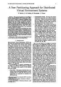
application command queues

OpenCL runtime CPU

GPU

Fig. 1: OpenCL in a heterogeneous environment. The user schedules task to command queues of which there is one for each device. The OpenCL run-time then breaks data-parallel task into chunks and sends them to the processing elements in the device.

The rest of this paper is structured as follows. Section 2 gives a brief introduction to OpenCL mapping and is followed in section 3 by a short example illustrating the performance impact of mapping decisions. Section 4 describes how we automatically build a partitioning model which is then evaluated in sections 5 and 6. Section 7 describes related work and is followed by some concluding remarks.

2

The OpenCL Programming Framework

Recent advances in the programmability of graphics cards have sparked a huge interest in what is now called general-purpose computing on graphics processing units or GPGPU. Several proprietary solutions like Brook [7] or NVIDIA CUDA [22] have been proposed, out of which the latter has arguably the greatest following. OpenCL is an attempt to develop an open alternative to these frameworks and is now being supported by most major hardware manufacturers. Furthermore, OpenCL not only targets GPUs, but entire heterogeneous systems including GPUs, CPUs and the Cell architecture. Due to its success, OpenCL’s programming model is similar to CUDA, focusing on data-parallelism. Data-parallel tasks are suitable for GPUs, in which groups of processing cores work in a SIMD fashion. In OpenCL, a data-parallel task is expressed as a kernel that describes the computation of a single workitem 1 . During program execution, a user-specified number of work-items is launched 1

A work-item is equivalent to a thread in CUDA.

to execute in parallel. These work-items are organized in a multi-dimensional grid and subsets of work-items are grouped together to form work-groups, which allow work-items to interact. Each work-item can query its position in the grid by calling certain built-in functions from within the kernel code. Despite OpenCL’s focus on data-parallelism, task-parallelism is also supported in the framework to allow execution on multiple devices, e.g. multiple GPUs or CPUs and GPUs.2 For each device, the user can create a command queue to which (data-parallel) tasks can be submitted (see figure 1). This not only allows the user to execute different tasks in parallel, but also enables decomposition of data-parallel tasks into sub-tasks that are distributed across multiple devices. Because OpenCL supports a variety of processing devices, all this can be achieved with just a single implementation of each task. Using CUDA a separate implementation for other devices, such as CPUs, would be needed. OpenCL’s memory model reflects the memory hierarchy on graphics cards. There is a global memory that is accessible by all work-items. There is also a small local memory for each work-group that can only be accessed by work-items from that particular work-group. Additionally, there is a constant memory which is read-only and can be used to store look-up tables, etc. This memory model is general enough to be mapped to many devices. Some processing devices, for example GPUs, have a global memory that is separate from the computer’s main memory. In this case, any data needs to be copied to the device and back to main memory before and after task execution, and can be a considerable overhead.

3

Motivation

Determining the right mapping for a task is crucial to achieve good performance on heterogeneous architectures. This section illustrates this point by examining the performance of three OpenCL programs, each of which needs a different partitioning to achieve its best performance. Figure 2 shows the speedup of three OpenCL programs with different mapping over single-core execution on a CPU. The specification of our system is provided in section 5.1. The x-axis shows how much of the program’s workload is executed on each device, i.e. the leftmost bar shows the speedup of GPU-only execution, one bar to the right shows the execution with 90% of work on the GPU and 10% on the CPUs and so on. For the coulombic potential program (figure 2a), a GPU-only execution achieves by far the best performance. Scheduling an amount of work as small as 10% to the CPUs leads to a slow-down of more than 5 times and this value increases if more work is mapped to the CPUs. For these types of programs it is absolutely vital to know ahead of time what the optimal mapping is, because a small mistake is going to be very costly. The matrix-vector multiplication program exhibits an entirely different behaviour (see figure 2b). The highest speedup is observed when 90% of the work 2

In OpenCL all CPU cores (even across multiple chips) are viewed as a single device.

16 12 8 4 0

/5

y

y

nl

nl

-o

0

PU

C

50

(a) coulombic potential (b) matrix-vector mult.

-o

y

nl

-o

0

y

nl work partitioning

PU

G

/5

PU

C

50

-o

y

y

nl

nl

-o

0

-o

PU

G

/5

PU

C

50

PU

G

work partitioning

8 6 4 2 0

Speedup

Speedup

Speedup

400 300 200 100 0

work partitioning

(c) convolution

Fig. 2: The speedup over single-core performance of three OpenCL programs with different partitions. The significant variations demonstrate the need for program-specific mappings.

is scheduled to the CPUs and only 10% to the GPU. The amount of computation per data item is fairly small and therefore the overhead of transferring data between main memory and the GPU’s memory is not worthwhile for large parts of the computation. The convolution program in figure 2c shows yet another different behaviour: A roughly even partitioning of work between CPUs and GPU leads to the best speedup. Unlike the other cases, neither a GPU-only nor a CPU-only execution would achieve good performance. As these programs have shown, a partitioning scheme that takes program characteristics into account is necessary to achieve good performance on heterogeneous systems. Different programs need different mappings and for some of them making a small mistake means that large potential speedups are missed. As OpenCL is a fairly new framework, compilers are likely to improve in the near future. The CPU implementation, in particular, seems to have much room for improvement. The next section describes our static partitioning approach based on static program code structure and machine-learning. By using machine-learning methods, our approach is portable across systems as well as implementations; a highly desirable property as program performance is likely to change across heterogeneous architectures and as OpenCL tools mature.

4

Partitioning Data-Parallel Tasks

Our approach uses machine-learning to predict the optimal partitioning for an OpenCL program solely based on compiler analysis of the program structure. The static analysis characterises a program as a fixed vector of real values, commonly known as features. We wish to learn a function f that maps a vector of program code features c to the optimal partitioning of this program, i.e. f (c) = p where p is as near as possible to the optimal partitioning. In order to map a task to the hardware without executing it, we need to analyse the code and extract code features. This section describes the static analysis framework used to extract code features at compile time. It also describes how

a machine-learning based model is built and then used to predict the optimal partitioning for any OpenCL program. Instead of relying on a single prediction model, we use hierarchical classification [5] where a hierarchy of models is evaluated to find the answer. As the models used are instances of support vector machines (SVMs) [8], we will also provide a brief introduction to SVMs. 4.1

Static Code Feature Extraction

Our partitioning method is entirely based on static code features eliminating the need for expensive off-line profiling [20] and also avoiding the pitfalls of dynamic techniques [24]. However, the features need to carry enough information to characterize the behaviour of OpenCL programs. In the following paragraphs we explain the feature extraction framework and describe the program code features used in the partitioning scheme. The compiler analysis is implemented in Clang [1], a C-language front-end for LLVM. The OpenCL program is read in by Clang which builds an abstract syntax tree. The analysis is based on a traversal of this tree, extracting code features such as the number of floating point instructions or the number of memory accesses in the program. Because many programs contain loops, we perform a value analysis to determine loop bounds (if possible). The value analysis is also used to analyze memory access patterns, which have a significant impact on performance on GPUs [26]. Memory accesses are called coalesced if adjacent work-items access adjacent memory locations. In this case multiple memory transfers can be coalesced into a single access increasing the overall memory bandwidth. This needs to be taken into account when mapping programs as it has a considerable impact on performance. The full list of static code features is shown in table 1. As indicated in the table, features describing absolute values are normalized. By multiplying the value by the number of work-items we compute the total number of operations for this program execution. Since a machine-learning model will not be able to relate two similar programs that have been executed with different input sizes, the total number of operations is divided by the data transfer size, to compute the number of operations per data item. In other words the normalized features are computed as operations in program code ×

number of work-items data transfer size

Before the features are passed to our model, we apply principal component analysis (PCA) [5] to reduce the dimensionality of the feature space and normalize the data (see section 4.2 for details). Our features describe both the computation and the memory operations of the kernel. First, it is important to describe the type and amount of computations (features 1-5). Some math operations, such as sine and cosine, can be mapped to special function units on some GPUs but may need to be emulated

Table 1: List of static code features used to characterize OpenCL programs and the corresponding values of the three example programs. 1 2 3 4 5 6 7 8 9 10 11 12 13

Static Code Feature cp mvm conv int operations (norm.) 31.6 0.6 28.8 int4 operations (norm.) 0 0 0 float operations (norm.) 1593.5 0.5 4.25 float4 operations (norm.) 0 0 0 intrinsic math operations (norm.) 249.9 0 0 barriers (norm.) 0 0.012 0.031 memory accesses (norm.) 0.125 0.5 2.6 percentage of local memory accesses 0 0.04 0.88 percentage of coalesced memory accesses 1 0.996 0 compute-memory ratio 15004 2.1 105.9 data transfer size 134249726 67141632 134217796 computation per data transfer 1875 1.6 35.7 number of work-items 2097152 4096 4194304

on CPUs, for example. Barriers (feature 6) may also cause different costs on different architectures. Second, memory operations (features 7-10) are important to consider. Depending on the architecture and type of memory the cost of memory accesses may vary. Accessing local memory on GPUs, for example, is cheap because it is mapped to small on-chip memory. On CPUs, however, local and global memory both get mapped to the same memory space. GPUs have a physically separate memory space and any data used during program execution needs to be copied to the GPU. The cost of data transfers between the memories is thus important. Features 11 and 12 capture the amount of memory to be transferred and how it compares to the amount of computation performed on the data. Lastly, feature 13 captures the overall size of the problem. Examples Table 1 shows the feature vectors for the example benchmarks introduced in section 3. The “computation to data transfer” ratio (feature 12), for example, is 1875 for the coulombic potential program, which is significantly higher than the value for convolution (35.7) and matrix-vector multiplication (1.6). The number of compute operations (features 1-5) and the ratio between compute- and memory-operations (feature 10) is also higher for coulombic potential compared to the others. These differences in input features reflect the different behaviours shown in figure 2. The optimal performance for the coulombic potential benchmark is achieved with GPU-only execution, because of the large number of compute-operations and the relatively small data transfer overhead. For the matrix-vector multiplication, on the other hand, very few operations are performed for each data item and the data transfer costs undo any potential speedups the GPU may offer. The feature values of the convolution bench-

mark are in-between the values of the other two programs. This explains why a more balanced work distribution is beneficial. 4.2

Building the Predictor

Building a machine-learning based model involves the collection of training data which is used to fit the model to the problem at hand. In our case, the training data consists of static code features of other OpenCL programs and the optimal partitioning of the corresponding program. This enables us to create a model that maps program code features to the program’s optimal partitioning. Rather than relying on an individual predictor, we combine several models to form a hierarchical classification model [5]. Collecting Training Data The training data for our model is divided into static code features (as described in section 4.1) and the optimal partitioning for the corresponding OpenCL program. The former will be the input for our model, whereas the latter is the output (or target) of our model. Each program is run with varying partitionings, namely all work on the CPU, 90% of work on the CPU and the remaining 10% on the GPU, 80% on the CPU and 20% on the GPU and so on. The partitioning with the shortest run-time is selected as an estimate of the optimal work partitioning for the program. Two-Level Predictor As was shown in section 3 OpenCL programs can be loosely divided into three categories, namely programs that achieve the best performance when (1) executed on GPU only (2) executed on CPUs only (3) partitioned and distributed over GPU and CPUs Getting the partitioning right is especially vital for programs in category 1. Not mapping all the work on the GPU leads to significant slowdowns (see Fig. 2a). Similarly (even though less drastic) for programs in category 2: If it is not worth copying the data back and forth to the GPU, one needs to make sure that the work is mapped to the CPU and any data transfer overhead is avoided. We therefore develop a prediction mechanism utilizing a hierarchy of predictors. This approach is known as hierarchical classification [5]. In the first level, programs from categories 1 and 2 are filtered out and mapped to the GPU or the CPUs, respectively. The remaining programs are mapped according to a third predictor in level 2 (see Fig. 3). The kernel features are reduced to two and eleven principal components using PCA for the first- and second-level predictors, respectively. Formally, we are mapping input features to one out of 11 classes, where class 0 represents GPU-only execution and class 10 CPU-only execution. Let gpu

kernel features stage 1 GPU-only?

execute on GPU only

CPU-only?

gpu && ¬cpu

cpu && ¬gpu

execute on CPU only

otherwise

stage 2

predict partitioning

Fig. 3: Overview of our prediction approach. Programs that should be entirely mapped to the GPU or to the CPUs are filtered out in the first level, while the second level handles programs that cannot be classified in level 1.

and cpu be the first-level predictors and hierarchical model can be described as   0 10 prediction(x) =  mix(x)

mix the second-level predictor. The if gpu(x) and ¬cpu(x) if cpu(x) and ¬gpu(x) otherwise

Level 1 predictors Focusing only on the extremes of the partitioning spectrum, the models in the first stage of the prediction are simple, but highly accurate (see section 6.2). One model predicts whether or not a program should be executed on the GPU only (category 1), while the other determines if a task is entirely mapped to CPUs (category 2). These “one-vs-all” classifiers [25] are implemented as binary classifiers based on a support vector machine (SVM) with a linear kernel (see section 4.4). Level 2 predictor If the first level of predictors does not lead to a conclusion, the program is passed on to another predictor. This one is more complex, because it needs to map a program to one out of the 11 classes determined during training. Again, we use an SVM-based model, but this time a radial basis function [5] kernel is deployed to account for the increased complexity of this problem. Whereas for the stage-1 models we use all of the available training data, we only use data from category 3 programs to train our model in the second level. This allows for the predictor to focus on programs whose optimal partitioning is likely to be neither CPU- nor GPU-only.

4.3

Deployment

At compile time, the program code is analyzed and code features are extracted. Because our model’s input features incorporate the task’s input size, the prediction cannot be made just yet. However, at run-time the input size is known and together with the previously extracted code features is passed to the model. The model’s output is the optimal partitioning for this program and input size which is used to partition the program between multiple devices. In OpenCL this can be easily done by setting a few variables. Although the prediction is done at run-time, the overhead is negligible as it only takes in the order of microseconds to evaluate our models; the cost of which is included in our later results. Examples Passing the features for the coulombic potential program as shown in figure 2a into our first-level predictors, we get a positive classification from the “GPU-only” predictor and a negative one from the “CPU-only” model. We therefore immediately map all of the computation to the GPU without evaluating the second level predictor. This leads to the optimal performance for this program. For the matrix-vector multiplication program, it is the other way around, i.e. we map the computation to the CPU only. Looking at figure 2b shows that while this is not the optimal partitioning we still achieve 98% of the optimum. With the convolution program, both first-level predictors say “no” and we move on to the second level predictor. Given the input features this model predicts that we should map 60% of the work to the GPU and the remaining 40% to the CPUs. According to figure 2c this leads to the optimal performance. 4.4

Support Vector Machines

Support Vector Machines (SVMs) [5] belong to the class of supervised learning methods and can be used for both classification and regression. The idea behind SVMs is to map the input feature space into a higher-dimensional space and then find hyperplanes that separate the training points from different classes. In the original feature space a linear separation may not be possible, but in a higher-dimensional space it is often easier to find such a separation. A new input feature vector is projected to the higher-dimensional space and a prediction is made depending on which side of the hyperplanes the projection is located. The projection into a higher-dimensional space is done using kernel functions. These include linear kernels or radial basis function kernels. Depending on the nature of the problem, some kernels perform better than others. A more detailed description of SVMs can be found in [5].

5 5.1

Methodology Experimental Setup

All experiments were carried out on a heterogeneous computer comprising two quad-core CPUs with Intel HyperThreading and an ATI Radeon HD 5970 GPU.

Table 2: Experimental Setup CPU GPU Architecture 2x Intel Xeon E5530 ATI Radeon HD 5970 Core Clock 2.4 GHz 725 MHz Core Count 8 (16 w/ HyperThreading) 1600 Memory Size 24 GB 1 GB Compiler GCC 4.4.1 w/ ”-O3” OS Ubuntu 9.10 64-bit OpenCL ATI Stream SDK v2.01

Table 2 shows more detailed information on our system as well as the software used. When the GPU was used, one CPU core was dedicated to managing the GPU. This has shown to be beneficial and is in line with observations made by Luk et al. [20]. Each experiment was repeated 20 times and the average execution time was recorded. In total we used 47 different OpenCL programs, collected from various benchmark suites: SHOC [9], Parboil3 [23], NVIDIA CUDA SDK [22] and ATI Stream SDK [2]. By varying the programs’ input sizes, we conducted a total of 220 experiments. We used the standard approach of cross-validation which has the critical property that when evaluating the model on a certain program, no training data from this program was used to build the model. 5.2

Evaluation Methodology

We compare our approach to an “oracle”, which provides an estimate of the upper bound performance. To find the oracle we tried all 11 partitions on the target program and selected the one with the lowest execution time. It may be possible that a partition that is not a multiple of 10% gives an even better speedup and thus our oracle is only an approximation. We further evaluate two default strategies: “CPU-only” and “GPU-only” simply map the entire work to the CPUs or to the GPU, respectively. These are two very primitive methods that serve as a lower bound in the sense that any partitioning scheme should (on average) beat them to prove itself useful. The fourth method we compare our approach against is a dynamic mapping scheme similar to what is presented by Ravi et al. [24], where the work of a kernel is broken into a certain number of chunks. Initially, one chunk is sent to the GPU and one to the CPUs. When either of them finishes, a new chunk is requested until the work is complete. We searched for the best number of chunks to divide the work into and found that using 8 chunks leads to the best overall performance on the set of kernels used in this paper, providing the right balance between scheduling overhead and flexibility. 3

The Parboil benchmark suite only contains CUDA programs. We therefore translated the benchmarks from CUDA to OpenCL. The OpenCL source code can be found at http://homepages.inf.ed.ac.uk/s0898672/opencl/benchmarks.html

The performance of each mapping technique is evaluated by computing the speedup over single-core execution. To collect the single-core run-times we used the same OpenCL code, but instructed the OpenCL run-time to only use one CPU core. This may underestimate the performance of a sequential version as it is likely to be faster than the parallel OpenCL code on a single core. However, as this value is used solely as a baseline to compare speedups of the competing techniques, it is appropriate for our purposes.

6

Results

In this section we show the performance of various mapping techniques. We compare our new approach with two static default strategies, namely “CPUonly” and “GPU-only”, as well as with the dynamic scheduling method described in section 5.2. The performance achievable with an optimal partitioning is also presented to compare the approaches to the maximal available speedups. This is followed by an evaluation of the accuracy of the various predictors in our model. 6.1

Speedup over Single-core Performance

We compare the run-times achieved with different partitioning schemes to the run-time on a single CPU core. Because of the large number of experiments we divided our programs according to the three categories described in section 4.2: Figure 4 shows programs where a “GPU-only” mapping achieves more than 90% of the optimal performance, whereas figure 5 shows programs where “CPU-only” achieves more than 80% of the optimum. The remaining programs are shown in figure 6. This not only helps understanding the results but also improves readability, as programs from different categories often have huge differences in speedup. GPU-friendly benchmarks Figure 4 shows the performance of the various techniques on OpenCL programs of category 1, i.e. programs that achieve the best speedups when executed on the GPU only. Unsurprisingly, the static “GPUonly” policy achieves near-optimal performance (compare to the right-most “oracle” bars). On these benchmarks this leads to an average speedup of 112 over single-core performance. Similarly obvious is that the “CPU-only” method clearly loses on these benchmarks, only achieving an average speedup of 8. The results for the dynamic approach are slightly better: Because the GPU is much faster than the CPUs on these programs, the majority of work will be scheduled to the GPU. However, some of the work is always scheduled to the CPUs which leads to significant slow-downs for most of the benchmarks when compared to the maximum performance. Overall, the dynamic scheduler achieves a speedup of 49. Our prediction approach, on the other hand, classifies almost all programs correctly and therefore achieves almost the same performance as the “oracle” scheduler with 113 times of the single-core performance.

CPU-only GPU-only

dynamic predictive model

oracle

Speedup over single-core

600 500 400 300 200 100 0

n ea m o Q ge q_ ri_m FH pb d_ fh rigy er _m en pb cu p_ ul M _c at pb _m dk T N _s _ nv m m ge n _s ca _s

sh

n ca

_s

sh l

ce

D

t1 iff

ac d_

_m

sh

l

a eg

a oc

_v

ar

dy

ft_ _f

sh

bo _n

st

hL

l_

C on

_m

st

ec

_d

Fi

ox _b

st

nc

_e

ES

ES

_A

st

_A

st

Fig. 4: Performance of those applications where the best speedup is achieved using only the GPU. Our predictive model leads to near-optimal performance compared to the oracle and a speedup of 2.3 over the dynamic scheme.

In our model, the majority of programs is filtered out by the first-level “GPUonly” predictor. Only very few are passed through to the next level. For those cases, the second-level predictor makes the right decision to schedule the work to the GPU. More detailed information on the accuracy of our model’s predictors will be shown in section 6.2. CPU-friendly benchmarks The performance of the different partitioning schemes on category 2 programs is shown in figure 5. This time around the static “CPUonly” policy achieves near-optimal performance. The average speedup equates to 6.12, only marginally below the upper bound of 6.36. Unsurprisingly the “GPU-only” method is worst for all programs, most of the time because shipping the data between main memory and GPU memory is not feasible. The average speedup of “GPU-only” is 1.05, i.e. no significant improvement over single-core execution can be observed. Again, the dynamic mapping method only comes second to last. The overhead of having many chunks and sending data to the GPU is simply too big to achieve good performance on these programs and leads to a speedup of only 2.15. Our prediction method comes close to the optimal performance. With an average speedup of 4.81 it is slower than the “CPUonly” policy on the CPU-friendly benchmarks, but significantly better than the dynamic scheme. This again shows our model’s high accuracy for partitioning OpenCL programs. Just like for the GPU-friendly programs, most of the CPUfriendly programs are filtered out in stage 1 of our prediction process. The few other programs are accurately mapped by the second-level predictor. For more detailed information on the predictors’ accuracies see section 6.2. Remaining benchmarks Performance results for all the remaining benchmarks are shown in figure 6. To improve readability, we have grouped the programs

CPU-only GPU-only

dynamic predictive model

oracle

Speedup over single-core

12 10 8 6 4 2 0

o ge 2

_c

ul

cM 1

_c

ul

0

_c

ul

cM

Ve

n ea

at

m

m

_ nv Ve

at

m

_ nv

1

0

nc

_u

ul

cM

Ve

at

m

_ nv cM

l

nc

_u

es

ul

cM

Ve

at

m

_ nv Ve

at

m ol ch

ba

lo

_g

6 25

m ra

og st

om

ks

At

st

ac bl

_ nv

_ nv

hi

_ st i _h

st

hi

_ st

Fig. 5: Performance of those applications where using only the CPU leads to almost optimal speedup. Our predictive model achieves a speedup of 2.2 over the dynamic scheme.

according to the maximum available speedup, i.e. programs in figure 6a achieve a larger speedup than programs in figure 6b. Both non-adaptive policies, “CPU-only” and “GPU-only”, do not do very well on most of these benchmarks, because the optimal performance is achieved when the work is distributed across both devices. On average, the “GPU-only” mapping achieves higher speedups (6.26 compared to 4.59), because the “CPUonly” policy misses out on potentially high speedups as shown in figure 6a. The dynamic scheme does reasonably well and achieves near-optimal performance for some benchmarks and an average speedup of 8.00. However, all schemes are outperformed by our prediction approach which achieves a speedup of 9.31 on average. Hence, even though the dynamic scheme shows its potential on these kind of programs, it is still outperformed by our prediction approach due to reduced scheduling overhead and more accurate work distribution. Summary As was shown in this section, a fixed partitioning that is agnostic to program characteristics is unsuitable for heterogeneous environments. The “CPU-only” and “GPU-only” methods only apply to a limited set of benchmarks and cannot adapt to different programs. Different programs need different mappings, highlighting the need for adaptive techniques. For the majority of programs, a partitioning of the work between CPUs and GPU is beneficial. While the dynamic partitioning method described in section 5.2 is designed to handle these cases, it is often unable to achieve good performance due to scheduling overhead and the inability to account for cases where a mixed execution is harmful. Our approach, in contrast, explicitly handles all cases and minimises overhead by making a static decision based on program code features.

CPU-only GPU-only

dynamic predictive model

oracle

140

Speedup over single-core

120 100 80 60 40 20 0

w ro v_ on l _c co nv v_ on N _c _N nv m m rm ge ifo _s un sh n_ ca _s sh 1D fft l2 ft_ ca o _f _l sh ul M al at oc _m _l st ul M at _m l st u M at t ro _m lb st de an _m st T C _D _h st t l Fi ox _b v lt_ Fi

st

s

le

ho sc

ck

ox _b

st

la _b

st

(a) CPU-only GPU-only

dynamic predictive model

oracle

16

Speedup over single-core

14 12 10 8 6 4 2 0

o

ge n

ea m

hi

ag

M

P ho

hi

d

_r

_p

od

or

hd

q ri-

f ri-

_m

pa

_m

pa Pr

ot

_d

nv

lo

co

ve

d_

_m

sh

s

us

al

ga

oc

t_

is

d un

bo

d_

_m

sh d_

w

T

AT

_l

m

to

sT

tA

er

_m

sh

is

_m

st

vS

lt_

0 AT

A hS

lt_

Fi

ox

_h

st

_b

st

hS

l_

Fi

ch

ar

l

Fi

ox

ox

_b

st

_b

st Fi

ox

Se

in

_b

st

_b

st

(b)

Fig. 6: Performance of those applications where a mix of both CPU- and GPUexecution leads to the best performance. Our predictive model achieves a speedup of 1.2 over the dynamic scheme and clearly outperforms both the CPUonly and GPU-only mapping.

Figure 7 shows the geometric mean over all benchmarks for the techniques presented in this paper. The “CPU-only” scheme is by far the worst technique because it does not adapt to programs and misses out on large speedups with GPU-friendly programs. Although the “GPU-only” mapping does not adapt to programs either, it achieves a better overall speedup because it correctly maps the programs that show high performance improvements over single-core execution. With an average speedup of 9.21 it is even marginally better than the dynamic method which achieves only 9.13 times the performance of single-

speedup over single-core

20

17.74 14.30

Speedup

15

10

5

9.21

9.13

GPU only

dynamic

4.73

0 CPU only

predictive model

oracle

Fig. 7: The average speedup (geometric mean) over all benchmarks. Our predictive modelling approach clearly outperforms all other competing techniques.

core execution. This again is because the potential of GPU-friendly programs is not realised. Our approach presented in this paper, on the other hand, leads to significantly higher speedups. With an average speedup of 14.30, we achieve more than 80% of the upper bound which equates to a speedup of 1.6 over the dynamic scheduler. 6.2

Prediction Accuracy

Let us take a closer look at the individual predictors in our model. Table 3 shows the number of applications that achieve the best performance with GPU-only and CPU-only execution respectively. The job of our two first-level predictors is to filter out these applications and to pass on the rest. Therefore, the table shows the numbers broken down according to the predictions in the first level of our model. Out of the 220 program-input pairs we examined, 61 should be entirely mapped to the GPU. 52 of those programs are identified by our first-level predictor and thus mapped to the GPU straightaway. The remaining 9 inputs are misclassified. However, they are passed on to the second-level predictor, which correctly maps them entirely to the GPU. 10 inputs are incorrectly classified as GPU-only and therefore mapped to the GPU although it is not optimal. However, in half of the cases this still leads to more than 90% of the optimal performance. Overall, the GPU-only classifier has an accuracy of 91%. 19 of the 23 program-input pairs that should be entirely mapped to CPUs are correctly classified by our second predictor in the first level of our model. For the 10 misclassified inputs we still achieve an average performance of 78% of the optimum. Overall, the CPU-only classifier achieves an accuracy of 95%.

Table 3: The accuracy of the binary classifiers in the first level our predictor. The “GPU-only” model achieves an accuracy of 91% while the “CPU-only” model even achieves a 95% accuracy. GPU ¬ GPU GPU predicted 52 10 ¬ GPU predicted 9 149

CPU ¬ CPU CPU predicted 19 6 ¬ CPU predicted 4 191

As expected, the second-level predictor has a lower accuracy than its counterparts in level 1. This is because its solving a much harder problem: instead of making a binary decision, one out of 11 classes needs to be predicted. However, being off by just one or two classes often still leads to good performance, on average a performance of 80% is still achieved. Our level 2 predictor is within these bounds for 65% of all programs. Looking at the model as a whole, we achieve an accuracy of 52%, i.e. in 52% of all program-input pairs we exactly predict the optimal mapping. This leads to an average 85% of the optimal performance, compared to only 58% of the dynamic partitioning method.

7

Related Work

The mapping or scheduling of tasks to heterogeneous systems is an extensively studied subject. In early publications, heterogeneous systems were often based on single-core CPUs running at different speeds. In 1977, for example, Ibarra et al. [13] described some of the first strategies for scheduling independent tasks to heterogeneous architectures. Given a function for each architecture that describes the run-time of a task on this processing unit they propose different heuristics to minimize the overall finishing time. In addition to those and other static techniques [6], several dynamic methods have been proposed [21, 29, 17]. On heterogeneous multi-core architecture consisting of multi-core CPUs and GPUs task mapping becomes more complex, because the devices are based on entirely different architectures. The tasks considered are also often data-parallel which means they can be split to use multiple devices concurrently. In the Harmony [10] framework programs are represented as a sequence of kernels. Whenever a kernel is available for execution it is dynamically scheduled to a device based on the suitability of the device for this kernel. The suitability is computed with a multivariate regression model that is built at run-time based on previous runs of the kernels. Harmony does not consider partitioning work and thus only schedules entire tasks. Qilin [20] also relies on a regression model to predict kernel run-times. In contrast to Harmony [10] which builds the model on-line, Qilin uses off-line profiling to create a regression model at compile time. Each kernel version is executed with different inputs and a linear model is fit to the observed run-times.

Rather than scheduling individual kernels, a single data-parallel task is split into sub-tasks which are each executed on one device. Qilin requires extensive offline profiling which may be prohibitive in some situations. Our approach, on the other hand, does not require any profiling and is entirely based on static code features. Merge [19] is a framework for developing map-reduce applications, i.e. programs comprised of data-parallel maps and reductions, on heterogeneous platforms. At run-time user-provided constraints are used to dynamically map subtasks to devices, favoring a more specific implementation over a more general implementation. In contrast to our scheme, they rely on the user to provide information on the suitability of a kernel for the devices. Ravi et al. [24] also propose a dynamic scheduling technique for map-reduce programs. Tasks are split into chunks that are then distributed across the devices similar to a master-slave model: When a device finishes processing a chunk of work, it requests a new one from a list of remaining work items. While the general idea of this model is straightforward, choosing the right chunk size has a non-negligible effect on performance as Ravi et al. show. However, they leave it for future work to predict the optimal chunk size. While purely dynamic approaches neither require user intervention nor profiling, they do not take any kernel characteristics into account which often leads to poor performance as shown in this paper. Jim´enez et al. [14] consider scheduling in multi-programmed heterogeneous environments. At run-time each program will be executed on all devices and the performance is collected. This information is then used to decide which processor a program will be executed on. A similar idea is proposed by Gregg et al. [12]. Based on the contention of devices and historical performance data they dynamically schedule programs to devices. Both methods do not consider partitioning tasks. StarPU [4] is a framework for programming on heterogeneous systems. The user provides multiple versions of each task and the run-time schedules them to the devices. Various scheduling techniques are presented, including greedy scheduling and performance-based scheduling. The performance estimations are either provided by the user or based on history information collected by the run-time [3]. Apart from Gregg et al. [12], none of the above approaches use OpenCL. While some use code generation from domain-specific high-level language representations, most of them rely on the user to provide separate kernel version for CPUs and GPUs. We circumvent this problem by using OpenCL which only requires a single kernel code version for both CPUs and GPUs.

8

Conclusion

This paper has developed a new approach for partitioning and mapping OpenCL programs on heterogeneous CPU-GPU systems. Given a data-parallel task, our technique predicts the optimal partitioning based on the task’s code features.

Our model relies on machine-learning techniques, which makes it easily portable across architectures and OpenCL implementations. This is a desirable property as both hardware and software implementations are going to evolve. When evaluated over 47 benchmark kernels, each with multiple input sizes, we achieve an average speedup of 14.3 over single-core execution. Compared to a state-of-the-art dynamic partitioning approach this equates to a performance boost of 1.57 times. Our approach also clearly outperforms the default strategies of using only the multi-core CPUs or only the GPU, which lead to a speedup of 4.73 and 9.21 over single-core execution, respectively. Future work will investigate the use of our partitioning and mapping technique for multi-kernel OpenCL programs. Furthermore, guided dynamic schemes will be explored that use kernel-specific information to improve the scheduling. This can be particularly useful in situations where a static, machine-learning based model has a low confidence of making the optimal decision, e.g. due to lack of training data.

References 1. Clang: a C language family frontend for LLVM. http://clang.llvm.org/, 2010. 2. AMD/ATI. ATI Stream SDK. http://www.amd.com/stream/, 2009. 3. C´edric Augonnet, Samuel Thibault, and Raymond Namyst. Automatic Calibration of Performance Models on Heterogeneous Multicore Architectures. In Euro-Par Workshops, 2009. 4. C´edric Augonnet, Samuel Thibault, Raymond Namyst, and Pierre-Andr´e Wacrenier. StarPU: A unified platform for task scheduling on heterogeneous multicore architectures. In Euro-Par, 2009. 5. Christopher M. Bishop. Pattern Recognition and Machine Learning (Information Science and Statistics). Springer-Verlag New York, Inc., Secaucus, NJ, USA, 2006. 6. Tracy D. Braun, Howard Jay Siegel, Noah Beck, Ladislau B¨ ol¨ oni, Muthucumaru Maheswaran, Albert I. Reuther, James P. Robertson, Mitchell D. Theys, Bin Yao, Debra A. Hensgen, and Richard F. Freund. A comparison study of static mapping heuristics for a class of meta-tasks on heterogeneous computing systems. In Heterogeneous Computing Workshop, 1999. 7. Ian Buck, Tim Foley, Daniel Reiter Horn, Jeremy Sugerman, Kayvon Fatahalian, Mike Houston, and Pat Hanrahan. Brook for GPUs: stream computing on graphics hardware. ACM Trans. Graph., 23(3), 2004. 8. Chih-Chung Chang and Chih-Jen Lin. LIBSVM: a library for support vector machines, 2001. Software available at http://www.csie.ntu.edu.tw/~cjlin/libsvm. 9. Anthony Danalis, Gabriel Marin, Collin McCurdy, Jeremy S. Meredith, Philip C. Roth, Kyle Spafford, Vinod Tipparaju, and Jeffrey S. Vetter. The scalable heterogeneous computing (SHOC) benchmark suite. In GPGPU, 2010. 10. Gregory F. Diamos and Sudhakar Yalamanchili. Harmony: an execution model and runtime for heterogeneous many core systems. In HPDC, 2008. 11. Romain Dolbeau, St´ephane Bihan, and Fran¸cois Bodin. HMPP: A hybrid multicore parallel programming environment. In Workshop on General Purpose Processing Using GPUs, 2007. 12. Chris Gregg, Jeff Brantley, and Kim Hazelwood. Contention-aware scheduling of parallel code for heterogeneous systems. Technical report, Department of Computer Science, University of Virginia, 2010.

13. Oscar H. Ibarra and Chul E. Kim. Heuristic algorithms for scheduling independent tasks on nonidentical processors. J. ACM, 24(2), 1977. 14. V´ıctor J. Jim´enez, Llu´ıs Vilanova, Isaac Gelado, Marisa Gil, Grigori Fursin, and Nacho Navarro. Predictive runtime code scheduling for heterogeneous architectures. In HiPEAC, 2009. 15. Ashfaq A. Khokhar, Viktor K. Prasanna, Muhammad E. Shaaban, and Cho-Li Wang. Heterogeneous computing: Challenges and opportunities. IEEE Computer, 26(6), 1993. 16. Khronos. OpenCL: The open standard for parallel programming of heterogeneous systems. http://www.khronos.org/opencl/, October 2010. 17. Jong-Kook Kim, Sameer Shivle, Howard Jay Siegel, Anthony A. Maciejewski, Tracy D. Braun, Myron Schneider, Sonja Tideman, Ramakrishna Chitta, Raheleh B. Dilmaghani, Rohit Joshi, Aditya Kaul, Ashish Sharma, Siddhartha Sripada, Praveen Vangari, and Siva Sankar Yellampalli. Dynamic mapping in a heterogeneous environment with tasks having priorities and multiple deadlines. In IPDPS, 2003. 18. Rakesh Kumar, Dean M. Tullsen, Norman P. Jouppi, and Parthasarathy Ranganathan. Heterogeneous chip multiprocessors. IEEE Computer, 38(11), 2005. 19. Michael D. Linderman, Jamison D. Collins, Hong Wang, and Teresa H. Y. Meng. Merge: a programming model for heterogeneous multi-core systems. In ASPLOS, 2008. 20. Chi-keung Luk, Sunpyo Hong, and Hyesoon Kim. Qilin: Exploiting parallelism on heterogeneous multiprocessors with adaptive mapping. In MICRO, 2009. 21. Muthucumaru Maheswaran and Howard Jay Siegel. A dynamic matching and scheduling algorithm for heterogeneous computing systems. In Heterogeneous Computing Workshop, 1998. 22. NVIDIA Corp. NVIDIA CUDA. http://developer.nvidia.com/object/cuda. html, 2010. 23. University of Illinois at Urbana-Champaign. Parboil benchmark suite, http:// impact.crhc.illinois.edu/parboil.php, 2010. 24. Vignesh T. Ravi, Wenjing Ma, David Chiu, and Gagan Agrawal. Compiler and runtime support for enabling generalized reduction computations on heterogeneous parallel configurations. In ICS, 2010. 25. Ryan M. Rifkin and Aldebaro Klautau. In defense of one-vs-all classification. Journal of Machine Learning Research, 2004. 26. Shane Ryoo, Christopher I. Rodrigues, Sara S. Baghsorkhi, Sam S. Stone, David B. Kirk, and Wen-mei W. Hwu. Optimization principles and application performance evaluation of a multithreaded GPU using CUDA. In PPoPP, 2008. 27. Sundaresan Venkatasubramanian and Richard W. Vuduc. Tuned and wildly asynchronous stencil kernels for hybrid CPU/GPU systems. In ICS, 2009. 28. Michael Wolfe. Implementing the PGI accelerator model. In GPGPU, 2010. 29. Vladimir Yarmolenko, Jos´e Duato, Dhabaleswar K. Panda, and P. Sadayappan. Characterization and enhancement of dynamic mapping heuristics for heterogeneous systems. In ICPP Workshops, 2000.