regularized pre-image. 1. INTRODUCTION. As a powerful quantitative imaging tool for tissue characterizations, MR parameter mapping has demonstrated.
ACCELERATING MR PARAMETER MAPPING USING NONLINEAR MANIFOLD LEARNING AND SUPERVISED PRE-IMAGING Yihang Zhou1, Chao Shi1, Fuquan Ren2, Jingyuan Lyu1, Dong Liang3 and Leslie Ying1, 4 1
Department of Electrical Engineering, State University of New York at Buffalo, Buffalo, NY, USA Department of Electrical and Electronic Engineering, Dalian University of Technology, Dalian, China 3 Paul C. Lauterbur Research Center for Biomedical Imaging, Shenzhen Institute of Advanced Technology, Shenzhen, China 4 Department of Biomedical Engineering, State University of New York at Buffalo, Buffalo, NY, USA 2
models over linear models for dynamic imaging applications [17][19]. The core concept of nonlinear model is to map the original signal space to a high dimensional feature space via a nonlinear function and seek the corresponding sparse representation of the mapped signal in the feature space. In this paper, we propose a novel framework to utilize nonlinear models to sparsely represent the unknown image. Different from the prior work with nonlinear models where the image series is reconstructed simultaneously, each image at a specific time point is assumed to lie in a lowdimensional manifold and is reconstructed individually. The low-dimensional manifold is learned from the training images generated by the parametric model. To reconstruct each image, among infinite number of solutions that satisfy the data consistent constraint, the one that is closest to the manifold is selected as the desired solution. The underlying optimization problem is solved using kernel trick [20] and split Bregman iteration algorithm [21]. Experimental results on T2 mapping using retrospectively undersampled data show that the proposed method is capable of recovering the T2 map at high reduction factors accurately when the conventional compressed sensing methods with linear models fail. This paper is structured as follows. In Section 2, we describe in details how the proposed method decouples the reconstruction process into two sequential steps: kernelbased manifold learning and regularized pre-imaging with data consistency and sparsity constraint. Section 3 evaluates the proposed method using in-vivo T2-weighted brain datasets. The paper is concluded in Section 4.
ABSTRACT In this paper, we propose a new reconstruction framework that utilizes nonlinear models to sparsely represent the MR parameter-weighted image in a high dimensional feature space. Different from the prior work with nonlinear models where the image series is reconstructed simultaneously, each image at a specific time point is assumed to lie in a low-dimensional manifold and is reconstructed individually. The low-dimensional manifold is learned from the training images generated by the parametric model. To reconstruct each image, among infinite number of solutions that satisfy the data consistent constraint, the one that is closest to the manifold is selected as the desired solution. The underlying optimization problem is solved using kernel trick and split Bregman iteration algorithm. The proposed method was evaluated on a set of in-vivo brain T2 mapping data set and shown to be superior to the conventional compressed sensing methods. Index Terms— MR parameter mapping, compressed sensing, nonlinear manifold learning, kernel PCA, regularized pre-image 1. INTRODUCTION As a powerful quantitative imaging tool for tissue characterizations, MR parameter mapping has demonstrated great potential in various clinical applications [1]. However, to accurately obtain the MR parameters values, a large amount of contrast-weighted images need to be acquired which can lead to a relatively long acquisition time that limits the practical utility of MR parameter mapping. A range of fast imaging techniques have been developed to accelerate the MR parameter mapping. These methods explicitly or implicitly use the parametric signal model and utilize various constraints associate with it. Typical examples include temporal smoothness constraint [3], sparsity or structured sparsity constraint [4]-[9], low rank constraint [10][11], contrast-weighting constraint [12]-[14], or a combination of them [15]-[17]. The above mentioned methods all use linear models for the constraints. In recent years, nonlinear models have been proposed in the compressed sensing framework and shown superiority on characterizing the nonlinearity in the signal
978-1-4799-2374-8/15/$31.00 ©2015 IEEE
2. PROPOSED METHOD 2.1 Problem Formulation To describe the data acquisition process, we represent the MR parameter-weighted image at the t-th acquisition to be reconstructed as an N 1 vector x. A finite number of measurements, denotes as y, are collected whose i-th entry can be written as (1)
y i x , f i i n
denotes the inner product, f i i 1 denotes i-th row of the undersampled Fourier measurement matrix F, and i denotes the complex white Gaussian noise. Since the where
897
measurement operation is under-determined, the direct recovery of x from measurement y is ill-posed. To reveal the nonlinear sparseness of the parameterweighted image x, we define a nonlinear mapping p q p : that maps the original data space into a much higher, even infinite, dimensional feature space q via a nonlinear function ( ) . We assume that x is nonlinearly d-sparse, meaning it can be sparsely represented by the first d largest coefficients in an orthonormal basis of the feature space q (x)
d k 1
whose rows are formed by Ti i 1 . solution of Eq. (5) is given by L
L
l (J l )
L
(4)
x
K i , j ( J i , J j ) ( J i ), ( J j ) with ( J i , J j ) being a
where c l
kernel function and is the eigenvalues of K. For simplicity, we assume that both ( J l ) and Κ are centered
K
c
with centered
T
L (x, V , U )
2.2 Nonlinear Manifold Learning In this step, we aim to find the projection coefficients
in the feature space q by solving
(8)
p
f
i 1
1
L l 1
(9)
c l (J l , f i ) f i
k l . To solve the optimization problem,
2
p
1 U
1 2
Fx y
2 2
2 2
1
2 V i 1 f
1
xVD
( 1)
D
(6)
1
2
c l (J l , f i ) f i
,
U HV
and
L l 1
F
(10)
V
2 1
2 2
2 2
p i 1
f
1
L l 1
U ΗV D
2
c l ( J l , f i ) f i 2
2
2
+ 3 U
F
(11)
1
( 1) 2
D 1 (V
( 1)
D 2 (Η V
x
( 1)
( 1)
U
)
( 1)
)
(12)
We now describe the three steps to be performed to solve Eq. (11).
where is a positive scalar and is the polynomial order, G MΛ
,
k
k 1
D1
where s i ( x , f i ) . Here we focus on a polynomial kernel
2
with
(5)
subject to V x ,
s G β δ.
2
2 (x) z
where V and U are called the auxiliary variables. Eq. (10) now can be solved iteratively by minimizing the cost function with respect to x, V and U separately using split Bregman algorithm without venturing into feature space [23]. Specifically, at the µ-th iteration, the scaled augmented Lagrangian function of Eq. (10) is
small number of projection coefficients β 1 , 2 , ..., d . Therefore, we propose the following two step sequential reconstruction scheme to recover x.
( x , f i ) ( x, f i ) ( y i )
d
2
x
Based on the above assumption, the desired MR parameter-weighted image x lies in a low dimensional manifold where the key information of x is preserved by a
T
arg m in F x y
Κ 1 L Κ Κ1 L 1 L Κ1 L .
β 1 , 2 , ..., d
1
we rewrite Eq. (8) as
in q . Otherwise we must replace ( J l ) with the centered ( J l ) ( J l ) l 1 J l L and replace Κ
1 Hx
2
invertible, and there is a unique solution to ( x ) z :
where Κ is a L L kernel matrix with the ( i , j ) th entry
L
2
where H denotes the two-dimensional finite difference operation matrix. The first term represents the data consistency, the second term exploits the sparsity constraint, and the third term enforces the solution to lie on the manifold spanned by the predefined feature space. Equation (8) can be highly nonlinear and nonconvex. However, when the polynomial kernel function has an odd order , the kernel function k ( x , f i ) f ( x, f i ) is
where ik i 1 is the representation coefficients that can be obtained by solving the following eigenvalue problem K k k
kvk .
x
(3)
k
k 1
arg min Fx y
generated beforehand based on the parametric model via kernel PCA (kPCA) [22]. Specifically, in kPCA, each q v k is represented in the expansion of L
d
2.3 Supervised Pre-Imaging The objective of this step is to find the desired image x in the original space, which is a pre-image of z [23][24], that is, ( x ) z . We also enforce that the pre-image satisfies the data consistency and transform sparse constraints. Therefore finding x is formulated as a supervised pre-image problem
the basis constructed using a set of training images J i i 1
l 1
space as z
q
(7)
Thereby we can obtain the unknown image in the feature
with β being the unknown coefficients, and v k k 1 being
vk
H
β (G G ) G s .
(2)
kvk
1
H
The least square
with M an n L matrix with the ( i , j ) th entries
defined as M i , j J j , f i and Λ is an L d matrix
x-step: Optimization with respect to x
In this step, Eq. (11) reduces to
898
x
( 1)
arg m in x
where ζ solution
( )
x
( )
V ( 1)
D
1
Fx y
2
.
( ) 1
2 2
2 2
xζ
( )
2
(13)
2
Eq. (13) has a closed-form
H 1 H ( ) F ( P 2 I ) F F u y 2 ζ .
(14)
where P is the undersampling pattern in k-space, and Fu P F .
V-step: Optimization with respect to V
In this step, Eq. (16) reduces to V
( 1)
arg m in V
1
2
x
2
( 1)
p
V i 1 f
2
1
( )
V D1
L l 1
2 2
2 2
c l (J l , f i ) f i
U
( )
2
( )
ΗV D 2
2
2
(15)
F
Taking the first order derivative of Eq. (15) with respect to V yields (x
( 1)
( )
T
V D 1 ) Η (U
where Q
p i 1
f
1
( )
L l 1
( )
HV D 2 )
1 2
(V Q ) 0
(16)
c l ( J l , f i ) f i . The solution to Eq.
(15) is given by
to get the best result and we chose 1 0.5 , 2 0.2 and 3 0.001 . Fig. 1 shows the reconstructed T2 maps and their corresponding pixel-wise error maps for white and gray matters only (CSF was removed through segmentation). The overall percentage errors are shown on the left top corner of the error maps. For better visualization, the error maps are magnified by 6. Visually the T2 maps obtained from the proposed method are indistinguishable from those obtained from the fully sampled data while the ones obtained from conventional CS reconstruction using linear PCA shows significant aliasing artifacts, especially in the white matter. We noticed that for the proposed method relatively higher error appears on the gray matter. This is likely due to the limited number of training images. Increasing the number of training images is expected to improve the reconstruction quality but at a cost of increased computational complexity. Another possibility is to improve the tissue segmentation so that the training images can be closer to the unknown image. To quantitatively assess our proposed method, the overall percentage errors were shown on the left top corner of the error maps. The results from the proposed method show good agreement with those from the fully sampled reference and are consistent for both undersampling factors of 4 and 8.
1
V
( 1)
( 1) ( ) T ( ) ( ) T x D 1 Η ( U D 2 ) 1 Q (1 1 ) I Η Η . 2 2
(17)
U-step: Optimization with respect to U
The last step we have to consider is U
( 1)
arg m in 3 U U
1
2 2
U ΗV
( 1)
( )
D2
2
as the gold standard for comparison between the proposed method and the conventional compressed sensing method with principle component analysis as the sparsifying transform (CS-PCA). All computations were carried out on a DELL workstation with Intel(R) i7 3.40GHz CPU and 16GB RAM running MATLAB 2012a (Mathworks, Natick, MA). The reconstruction time is about 210s for the proposed method and 90s for CS-PCA. As previously stated, the proposed method requires training images to estimate the basis function in the feature space. The k-space at the second echo time was fully sampled and used to form a reference image ρ. Similar to MR fingerprinting [25], tissue classification was achieved by segmenting the reference image. In our current implementation, the segmentation was performed by grouping regions with similar intensities although other advanced segmentation methods could be applied to further improve the segmentation. The training images were then generated using ρ e ( TE / T 2 ) with a number of possible T2 values based on the segmentation of different tissues at each TE. A total of 976 training images were generated for each echo time. We used the polynomial kernel with 1 5 and 5 . The regularization parameters were manually tuned
. (18)
This is a typical L1 minimization problem which can be easily solved by any off-the-shelf optimization method. Finally, by iterating through the abovementioned three steps we may accurately recover the desired MR parameter weighted image x from the t-th acquisition. 3. EXPERIMENTS AND RESULTS We evaluate the proposed method using T2 mapping experiments, where the signal is described by an exponential decay. However, the method can be generalized for any other parameter mapping models. A set of brain data was acquired on a 3T scanner using a 12-channel head coil with a turbo spin echo sequence (matrix size = 192 × 192, FOV = 192 × 192 mm, slice thickness = 3.0 mm, ETL = 16, ΔTE = 8.8 ms, TR = 4000 ms, bandwidth = 362 Hz/pixel). The kspace obtained at the first echo time was not used due to its hypointense. To simulate the reduced acquisition retrospectively, the k-space data was randomly undersampled along the phase encoding direction at each echo time with net reduction factors of 4 and 8, respectively. Different sampling patterns were used at different TEs. The T2 map obtained by pixel-wise fitting using the LevenbergMarquardt algorithm from the fully sampled data was used
4. CONCLUSION In this paper, a novel reconstruction method is proposed to accelerate the MR quantitative imaging. Compared to the existing compressed sensing methods, the proposed method constrains both the linear and nonlinear sparsity of the images using nonlinear manifold learning and supervised pre-imaging. The underlying optimization problem is solved by kernel trick and split Bregman algorithm. Experimental
899
results show that the proposed method can accurately recover MR parameter maps from highly undersampled datasets. Future work will investigate selection of kernel functions and evaluation on other MR parametric models.
[6] [7]
5. ACKNOWLEDGMENT This work was supported in part by the National Science Foundation CBET-1265612. CS-PCA
FS
[8] [9]
Proposed
[10]
R=4
[11] [12] 10.31%
4.19%
[13] [14] x6
x6
R=8
[15]
[16] 15.71%
6.68%
[17] [18]
x6
0
50
100
150
200
x6
250
[19]
300 [20]
[21]
6. REFERENCES
[22]
[1] H.-L. Margaret Cheng, N. Stikov, N. R. Ghugre, and G. A. Wright, “Practical medical applications of quantitative MR relaxometry,” J. Magn. Reson. Imag., 2012; 36: pp. 805–824, 2012. [2] M. Lustig, D.L. Donoho, and J.M. Pauly, “Sparse MRI: The application of compressed sensing for rapid MR imaging,” Mag. Reson. Med. 2007, 58: pp. 1182–1195. [3] J.V. Velikina, A. L. Alexander, A. Samsonov, “Accelerating MR parameter mapping using sparsity-promoting regularization in parametric dimension,” Magn. Reson. Med. 2013; 70:1263–1273. [4] M. Doneva, P. Bornert, H. Eggers, C. Stehning, J. Senegas, A. Mertins, “Compressed sensing reconstruction for magnetic resonance parameter mapping,” Magn. Reson. Med. 2010; 64:1114–1120. [5] L. Feng, R. Otazo, H. Jung, J. H. Jensen, J.C. Ye, D. K. Sodickson, D. Kim, “Accelerated cardiac T2 mapping using
[23] [24] [25]
900
breath-hold multiecho fast spin-echo pulse sequence with k-t FOCUSS,” Magn. Reson. Med. 2011; 65:1661–1669. Bilgic B, Goyal VK, Adalsteinsson E. “Multi-contrast reconstruction with Bayesian compressed sensing,” Magn. Reson. Med. 2011; 66:1601–1615. A. Majumdar, R. K. Ward, “Accelerating multi-echo T2 weighted MR imaging: analysis prior group-sparse optimization,” J. Magn. Reson. Imaging. 2011; 210:90–97. J. Yuan, D. Liang, F. Zhao, Y. Li, Y.-X. Xiang, L. Ying, “k-t ISD compressed sensing reconstruction for T1 mapping: a study in rat brains at 3T,” in Proc. ISMRM 2012. p. 4197. J. Huang, C. Chen, L. Axel, “Fast multi-contrast MRI reconstruction,” in Proc. 15th MICCAI 2012. pp. 281–288. F. H. Petzschner, I. P. Ponce, M. Blaimer, P. M. Jakob, F. A. Breuer. Fast MR parameter mapping using k-t principal component analysis. Magn. Reson. Med. 2011; 66:706–716. T. Zhang, J. M. Pauly, I. R. Levesque, “Accelerating parameter mapping with a locally low rank constraint,” in press, Magn. Reson. Med. 2014. J. P. Haldar, D. Hernando, Z.-P. Liang, “Super-resolution reconstruction of MR image sequences with contrast modeling,” In Proc. ISBI, 2009. pp. 266–269. K. Block, M. Uecker, J. Frahm, “Model-based iterative reconstruction for radial fast spin-echo MRI,” IEEE Trans. Med. Imaging 2009; 28:1759–1769. T. J. Sumpf, M. Uecker, S. Boretius, J. Frahm, “Model-based nonlinear inverse reconstruction for T2 mapping using highly undersampled spin-echo MRI,” J. Magn. Reson. Imaging. 2011; 34:420–428. C. Huang, C. G. Graff, E. W. Clarkson, A. Bilgin, M. I. Altbach, “T2 mapping from highly undersampled data by reconstruction of principal component coefficient maps using compressed sensing,” Magn. Reson. Med. 2012; 67: 1355–1366. B. Zhao, W. Lu, T. K. Hitchens, F. Lam, C. Ho and Z.-P. Liang, “Accelerated parameter mapping with low rank and sparsity constraints,” Magn. Reson. Med.2014: early view. B. Zhao, F. Lam, Z.-P. Liang, “Model-based MR parameter mapping with sparsity constraints: parameter estimation and performance bounds,” IEEE Trans. Med. Imaging 2014: in press. Y. Zhou, Y. Wang, L. Ying, “A kernel-based compressed sensing approach to dynamic MRI from highly undersampled data,” In Proc. ISBI, 2013, pp. 310-313. Y. Wang, L. Ying, “Undersampled Dynamic Magnetic Resonance Imaging using Kernel Principal Component Analysis,” In Proc. IEEE EMBC, 2014 pp.1533-1536. H. Qi and S. Hughes, “Using the kernel trick in compressive sensing: Accurate signal recovery from fewer measurements,” in Proc. 2011 IEEE Int. Conf. Acoust., Speech, Signal Process., pp. 3940-3943. N. Nguyen, J. Chen, C. Richard, P. Honeine, and C. Theys. “Supervised nonlinear unmixing of hyperspectral images using a pre-image methods,” EAS Publications Series 2013, 59, 417-437. B. Scholkopf, A. Smola, and K.R. Muller, “Kernel principal component analysis,” in Proc. 1997 ICANN LNCS, pp. 583-588. B. Schlkopf and A. J. Smola, “Learning with kernels: support vector machines, regularization, optimization, and beyond,” MIT Press, Boston, 2001. S. Mika, B. Schölkopf, A. Smola, K.L. Müller , M. Scholz, and G. Rätsch, “Kernel PCA and de-noising in feature spaces,” Adv. Neural. Inf. Process. Syst., vol. 11, pp. 536-542, 1999. D. Ma, V. Gulani, N. Seiberlich, K. Liu, J. L. Sunshine, J. L. Duerk, and M. A. Griswold. Magnetic resonance fingerprinting. Nature 2013, 495(7440): pp. 187-192.