polynomials which we then use to further test all three gp variants. 1 Introduction ..... 200 generations and by gp-csaw in experiment 5 within 100 generations.
Adaptive Genetic Programming Applied to New and Existing Simple Regression Problems Jeroen Eggermont and Jano I. van Hemert Leiden Institute of Advanced Computer Science, Leiden University {jeggermo,jvhemert}@cs.leidenuniv.nl
Abstract. In this paper we continue our study on adaptive genetic programming. We use Stepwise Adaptation of Weights (saw) to boost performance of a genetic programming algorithm on simple symbolic regression problems. We measure the performance of a standard gp and two variants of saw extensions on two different symbolic regression problems from literature. Also, we propose a model for randomly generating polynomials which we then use to further test all three gp variants.
1
Introduction
We test a technique called Stepwise Adaptation of Weights (saw) on symbolic regression. We use a genetic programming algorithm and adapt its fitness function using the saw technique in an attempt to improve both algorithm performance and solution quality. Also, we present a new variant of the saw technique called Precision saw. Previous studies on constraint satisfaction [6] and data classification [4] have indicated that saw is a promising technique to boost the performance of evolutionary algorithms. It uses information of the problem from the run so far to adapt the fitness function of an evolutionary algorithm. In a regression problem we are looking for a function that closely matches an unknown function based on a finite set of sample points. Genetic programming (gp) as introduced by Koza [9] uses a tree structure to represent an executable object or model. Here we will use gp to search for functions that solve a symbolic regression problem. The next section defines the symbolic regression problem and how this is solved using genetic programming. In Sect. 3 we provide information on the saw technique and show how this technique can be applied to symbolic regression. In Sect. 5 we explain our experiments and we provide results. Finally we draw conclusions and we provide ideas for further research.
2
Symbolic Regression with Genetic Programming
The object of solving a symbolic regression problem is finding a function that closely matches some unknown function on a certain interval. More formally, given an unknown function f (x) we want to find a function g(x) such that
f (xi ) = g(xi ) ∀xi ∈ X, where X is a set of values drawn from the interval we are interested in. Note that we normally do not know f (x) precisely. We only know the set of sample points {(x, f (x))|x ∈ X}. In this study we use predefined functions and uniformly draw a set of 50 sample points from it to test our regression algorithms equivalent to the experiments with these functions in [10]. We use a genetic programming algorithm to generate candidate solutions, i.e., g(x). These functions are presented as binary trees built up using binary functions and a terminal set. The precise definition of these sets and other parameter settings varies between the two experiments presented later. Therefore, we defer the presentation of these parameters until Sect. 5 where we conduct our experiments. The selection scheme in an evolutionary algorithm is one of its basic components. It needs a way to compare the quality of two candidate solutions. This measurement, the fitness function, is calculated using knowledge of the problem. In symbolic regression we want to minimise the total error over all samples. This is defined as the absolute error in (1), which will be the fitness function for the standard gp algorithm. X �= |f (x) − g(x)| (1) x∈X
Other fitness functions can be used. For instance, based on the mean square error. We use this simple approach and make it adaptive in the next section.
3
Stepwise Adaptation of Weights
The Stepwise Adaptation of Weights (saw) technique was first studied on the constraint satisfaction problem (csp). Solving a csp can mean different things. Here the object is to find an instantiation of a set of variables such that none of the constraints that restrict certain combinations of variable instantiations are violated. This is a np-hard problem on which most evolutionary computation approaches will fail because they get stuck in local optima. The saw technique is designed to overcome this deficiency. In data classification the problem is to find a model that can classify tuples of attributes as good as possible. When we observe this problem with constraint satisfaction in mind we can draw some analogies. For instance, in csp we have to deal with constraints. Minimising the number of violated constraints is the object and having no violated constraints at all yields a solution. Similarly, in data classification, minimising the number of wrongly classified records is the object, while correctly classifying all records yields a perfect model. The idea of data classification can further be extended to symbolic regression. Here we want to find a model, i.e., a function, that correctly predicts values of the unknown function on the sampled points. The object is minimising the error of prediction, consequently having no error means having found a perfect fit. This is where saw steps into the picture by influencing the fitness function of an evolutionary algorithm. Note that in all the problems mentioned above the fitness has to be minimised to reach the object. The idea behind saw is to
adapt the fitness function in an evolutionary algorithm by using knowledge of the problem in the run so far.
Algorithm 1 Stepwise adaptation of weights (saw) set initial weights (thus fitness function f ) set G = 0 while not termination do G=G+1 run one generation of gp with f if G ≡ 0 (mod ∆T ) then redefine f and recalculate fitness of individuals fi end while
The general mechanism for saw is presented in Figure 1. The knowledge of the problem is represented in the form of weights. We add a weight wi to every sample point xi ∈ X. These weights are initially set to one. During the run of the genetic programming algorithm we periodically stop the main evolutionary loop every ∆T generations and adjust the weights by increasing them. Afterwards, we continue the evolutionary loop using the new weights incorporated into the fitness function as shown in (2). X saw fitness(g, X) = wi |f (xi ) − g(xi )| (2) xi ∈X
The adaptation of weights process takes the best individual from the current population and determines the error it makes on each sample point. Each of the weights wi corresponding to the error made on point xi is updated using the error value |f (xi ) − g(xi )|. We try two variants for altering weights. – Classic saw (csaw) adds a constant value ∆wi = 1 to each wi if the error on sample point xi is not zero. This is based on the approach of violated constraints [6]. – Precision saw (psaw) takes ∆wi = |f (xi ) − g(xi )| and adds ∆wi to the corresponding weight wi .
4
Problem generator
Besides testing our two gp variants on two problems taken from literature we present here a method for generating symbolic regression problems. This enables us to study the performance of these techniques on a large set of polynomials of a higher degree. The regression of higher degree polynomials finds its use in different application areas such as computer vision and economics [2]. We generate the polynomials using a model of two integer parameters ha, bi, where a stands for the highest possible degree and b determines the domain size
from which every ei is chosen. When we have set these parameters we are able to generate polynomials in the form as shown in (3). The values ei are drawn uniform random from the integer domain bounded by −b and b. a X
� ei xi , where ei ∈ {w|w ∈ Z ∧ −b ≤ w ≤ b}
(3)
i=0
The function f (x) is presented to the regression algorithms by generating 50 points (x, f (x)) uniformly from the domain [−1, 1]. This method for generating X will also be used for the two Koza functions [10].
5 5.1
Experiments and Results Koza functions
To test the performance of the two variants of saw we do a number of experiments using three algorithms. First, the genetic programming algorithm without any additional aids (gp). Second, the variant where we add saw with a constant ∆w (gp-csaw). Last, the variant where we add saw with ∆wi = |f (xi ) − g(xi )| (gp-psaw). We measure performance of the algorithms on two simple symbolic regression problems. Each algorithm is tested with two different population sizes as shown in Table 1. We use 99 independent runs for each setting in which we measure mean, median, standard deviation, minimum and maximum absolute error (�). Furthermore we count the number of successful runs. Where we define a run successful if the algorithm finds a function that has an absolute error below 10−6 . Besides comparing the three genetic programming variants we also provide results obtained by using splines on the same problems. This places our three algorithms in a larger perspective. Table 1. Experiment parameters: six different experiments where each experiment consists of 99 independent runs experiment
populations size
number of generations
1 2 3 4 5 6
100 100 100 100 500 500
100 200 500 1000 100 200
Here we present two experiments with functions taken from [10]. All genetic programming systems used the parameters shown in Table 2.
Table 2. Parameters and characteristics of the genetic programming algorithms for experiments with the Koza functions parameter
value
evolutionary model (µ, 7µ) fitness standard gp see (1) fitness saw variants see (2) stop criterion maximum generations or perfect fit functions set {∗, pdiv, −, +} terminal set {x} populations size see Table 1 initial depth 3 maximum depth 5 maximum generations see Table 1 survivors selection keep best populations size offspring parent selection random ∆T (for saw) 5
f(x)
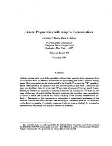
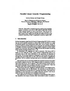
Quintic polynomial This quintic polynomial is taken from [10] and is defined by (4). The function is shown in Fig. 1. When we try to regress this function using standard cubic regression we get a total error (as measured with �) of 1.8345. f (x) = x5 − 2x3 + x, x ∈ [−1, 1] (4)
-1
-0.5
0 x
0.5
1
Fig. 1. The quintic polynomial on the interval [−1, 1] (left)
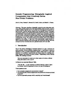
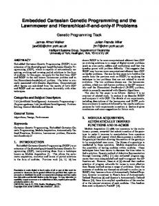
Table 3 shows the results of the experiments on the quintic polynomial. Looking at the mean and the median for all experiments we conjecture that gp-psaw produces the best solutions. gp-csaw is not always better than gp, but it has the best results when we observe the maximum error, i.e., the worst result found. The best solution (1.704 × 10⁻⁷ ) is found twice by gp-csaw. We look at the individual runs of experiment 4 (population size of 100 and 1000 generations) and determine all the successful runs and see that gp has 76
Standard fitness of best indivdual
10
GP GP+CSAW GP+PSAW
1 0.1 0.01 0.001 0.0001 1e-05 1e-06 1e-07 100
1000
10000 100000 Evaluations
1e+06
Fig. 2. Absolute error (�) over evaluations for one run of the three algorithms for the quintic polynomial (right)
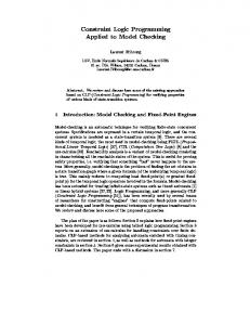
successful runs out of 99, gp-csaw has 78 successful runs out of 99 and gp-psaw has 85 successful runs of 99. These result are set out in Fig. 3 together with their uncertainty interval [13]. We use the usual rule of thumb where we need at least a difference two and a half times the overlap of the uncertainty interval before we can claim a significant difference. This is clearly not the case here. In experiment 6 (population size 500 and 200 generations) gp fails 2 times out of 99. The other two algorithms never fail. This is a significant difference, albeit a small one as the uncertainty intervals still overlap. Sextic polynomial This sextic polynomial is taken from [10] and is defined in (5). Figure 4 shows this function on the interval [−1, 1]. When we do a cubic regression on the function we get a total error (measured with �) of 2.4210. f (x) = x6 − 2x4 + x2 , x ∈ [−1, 1]
(5)
Table 4 shows the results of the experiments on the sextic polynomial. gppsaw has the best median in one experiment and best mean in three experiments. gp-csaw never has the best mean but has the best median three times. If we are only interested in the best solution over all runs we have an easier job comparing. The best solution (1.013 × 10⁻⁷ ) is found in experiment 2 by gp-psaw in just 200 generations and by gp-csaw in experiment 5 within 100 generations.
Table 3. Experiment results for the quintic polynomial, all measurements taken with absolute error (�) experiment median (×10−7 )
mean (×10−1 )
stddev minimum (×10−1 ) (×10−7 )
maximum
1. gp gp-csaw gp-psaw
4.610 4.605 4.391
1.351 1.339 1.286
2.679 2.599 2.972
2.640 2.445 2.598
1.050 1.102 1.559
2. gp gp-csaw gp-psaw
4.354 4.303 4.200
1.274 1.226 1.049
2.610 2.376 2.254
2.640 2.445 2.543
1.034 0.8525 1.317
3. gp gp-csaw gp-psaw
3.972 4.019 3.855
1.120 1.107 0.7785
2.571 2.204 2.049
2.640 1.704 2.449
1.034 0.8525 1.111
4. gp gp-csaw gp-psaw
3.763 3.693 3.669
1.161 0.8323 0.6513
2.547 1.803 1.856
2.324 1.704 2.114
1.034 0.6969 1.111
5. gp gp-csaw gp-psaw
3.465 3.465 3.395
2.045×10⁻¹ 3.570×10⁻⁵ 3.382×10⁻⁵
1.544×10⁻² 8.463×10⁻⁸ 4.384×10⁻⁸
1.965 2.412 1.974
1.433×10⁻¹ 9.965×10⁻⁷ 5.071×10⁻⁷
6. gp gp-csaw gp-psaw
3.343 3.446 3.325
2.045×10⁻¹ 3.512×10⁻⁵ 3.331×10⁻⁵
1.544×10⁻² 8.337×10⁻⁸ 4.533×10⁻⁸
1.965 2.412 1.937
1.433×10⁻¹ 9.965×10⁻⁷ 5.071×10⁻⁷
Table 4. Experiment results for the sextic polynomial, all measurements taken with absolute error (�) experiment median (×10−7 )
mean (×10−1 )
stddev minimum (×10−1 ) (×10−7 )
maximum
1. gp gp-csaw gp-psaw
2.182 2.182 2.182
1.490 1.525 1.212
3.987 4.036 2.569
1.723 1.353 1.213
2.844 2.844 1.720
2. gp gp-csaw gp-psaw
2.182 2.098 2.115
1.179 1.244 1.135
2.882 3.626 2.495
1.172 1.244 1.013
1.730 2.491 1.720
3. gp gp-csaw gp-psaw
1.953 1.916 1.984
0.8001 0.8366 0.8403
2.318 2.328 2.226
1.171 1.172 1.013
1.730 1.222 1.720
4. gp gp-csaw gp-psaw
1.888 1.824 1.899
0.6963 0.6100 0.5084
2.258 1.741 1.418
1.135 1.048 1.013
1.730 1.161 5.467×10⁻¹
5. gp gp-csaw gp-psaw
1.385 1.385 1.385
1.507×10⁻⁶ 3.390×10⁻² 2.485×10⁻²
3.280×10⁻⁷ 2.500×10⁻¹ 2.460×10⁻¹
1.087 1.013 1.125
2.912×10⁻⁷ 2.255×10⁻¹ 2.460×10⁻¹
6. gp gp-csaw gp-psaw
1.260 1.363 1.260
1.417×10⁻⁶ 3.390×10⁻² 2.485×10⁻²
3.029×10⁻⁷ 2.500×10⁻¹ 2.460×10⁻¹
1.087 1.013 1.115
2.912×10⁻⁷ 2.255×10⁻¹ 2.4560×10⁻¹
GP
GP
GP+CSAW
GP+CSAW
GP+PSAW
GP+PSAW 60
65
70 75 80 85 90 95 100 Number of successful runs
90
92 94 96 98 Number of successful runs
100
f(x)
Fig. 3. Number of successful runs with uncertainty intervals for the quintic polynomial in experiment 4 (left) and experiment 6 (right)
-1
-0.5
0 x
0.5
1
Fig. 4. The sextic polynomial on the interval [−1, 1]
Similar to the quintic polynomial we examine the individual runs of experiment 4 (population size of 100 and 1000 generations) and determine all the successful runs. Here gp has 84 successful runs out of 99. gp-csaw has 81 successful runs and gp-psaw has 87 successful runs. These result are set out in Fig. 6 together with the uncertainty interval [13]. Although differences seem larger than with the quintic polynomial we still cannot claim a significant improvement. Tides turn compared to the quintic polynomial as here gp-csaw fails twice, gp-psaw fails once and gp always succeeds. This leads to a significant difference with overlapping uncertainty intervals between gp and gp-csaw.
5.2
Randomly generated polynomials
Here we test our three gp variants on a suite of randomly generated polynomials. These polynomials can have at most a degree of twelve. The parameters of the underlying gp system are noted in Table 5
Standard fitness of best indivdual
10
GP GP+CSAW GP+PSAW
1 0.1 0.01 0.001 0.0001 1e-05 1e-06 1e-07 100
1000
10000 100000 Evaluations
1e+06
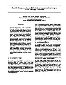
Fig. 5. Absolute error (�) over evaluations for one run of the three algorithms for the sextic polynomial (right)
We generate polynomials randomly with the model from Sect. 4 with parameters h12, 5i. We generate 100 polynomials and do 85 independent runs of each algorithm where each run is started with a unique random seed. The previous simple functions had a smaller maximum degree and could therefore be efficiently solved with cubic splines. Here we need a technique that can handle a higher degree of polynomials. Hence, we try a curve fitting algorithm that uses splines under tension [3] on every generated polynomial. The results are very good as the average total error over the whole set of polynomials measured as the absolute error (�) is 1.3498346 × 10⁻⁴ . We present the results for the set of randomly generated polynomials in Table 6. Clearly, the new variant gp-psaw is better than any of the others as long as we do not update the saw weights too many times. This seems like a contradiction as we would expect the saw mechanism to boost improvement, but we should not forget that after updating the weights the fitness function has changed so we need to re-calculate the fitness for the whole population. This re-calculateion can be performed by either re-evaluating all individuals or by using a cache-memory which contains the predicted value for each point and individual. Because we have used a general library we opted for the re-evaluation. Also, when we would extend the system in such a way that the data points would change during the run this would render the cache useless. But, in a gp system
GP
GP
GP+CSAW
GP+CSAW
GP+PSAW
GP+PSAW 60
65
70 75 80 85 90 95 100 Number of successful runs
90
92 94 96 98 Number of successful runs
100
Fig. 6. Number of successful runs with uncertainty intervals for the sextic polynomial in experiment 4 (left) and experiment 6 (right)
Table 5. Parameters and characteristics of the genetic programming algorithms for experiments with the random polynomials parameter
value
evolutionary model steady state (µ + 1) fitness standard gp see (1) fitness saw variants see (2) stop criterion maximum evaluations or perfect fit functions set {∗, pdiv, −, +, ¬, y 3 } terminal set {x} ∪ {w|w ∈ Z ∧ −b ≤ w ≤ b} populations size 100 initial maximum depth 10 maximum size 100 nodes maximum evaluations 20,000 survivors selection reverse 5-tournament parent selection 5-tournament ∆T (for saw) 1000, 2000 and 5000 generations
this will cost us fitness evaluations, leaving less fitness evaluations for the gp. Thus less points of the problem space are visited. The comparison with the splines on tension only remains. The error of the splines on tension is incredibly low. As such our results are significantly worse. One reason could be the number of evaluations that are performed at maximum. Here we have set this at 20,000. If we look at the right hand of Figure 4 we notice that the absolute error suddenly drops after 10,000 evaluations. If we take into account that our current polynomials have a degree that is up to twice that of the sextic polynomial we can expect that a better solution will not be found before this 20,000 mark.
Table 6. Experiment results for 100 randomly generated polynomials, results are averaged over the 85 independent runs. The error is measured as absolute error (1)
6
algorithm
∆T
mean
stddev
minimum
maximum
gp gp-csaw gp-csaw gp-csaw gp-psaw gp-psaw gp-psaw
1000 2000 5000 1000 2000 5000
21.20 21.55 21.21 21.25 21.46 20.45 20.28
10.30 10.33 10.24 10.47 10.52 10.05 9.87
5.82 5.79 5.83 5.75 6.41 5.90 5.96
48.60 48.05 48.74 49.31 50.80 48.06 48.18
Conclusions
We have shown how the saw technique can be used to extend genetic programming to boost performance in symbolic regression. We like to point out that the simple concept behind saw makes it very easy to implement the technique in existing algorithms. Thereby, making it suitable for doing quick try outs to boost an evolutionary algorithms performance. As saw solely focuses on the fitness function it can be used in virtually any evolutionary algorithm. However, it is up to the user to find a good way of updating the weights mechanism depending on the problem at hand. This paper shows two ways in which to add saw to a genetic programming algorithm that solves symbolic regression problems. By doing this, we add another problem area to a list of problems that already contains various constraint satisfaction problems and data classification problems. When we focus on a comparison of mean, median and minimum fitness it appears that our new variant of the saw technique (Precision saw) has the upper hand. In most cases it finds a better or comparable result than our standard gp, also beating the Classic saw variant. Moreover, it seems that the saw technique works better using smaller populations. Something that is already concluded by Eiben et al. [5]. When we restrict our comparison to the number of successes and fails we find that there is only a small significant difference when we run the algorithms with a populations size of 500. Then gp+psaw is the winner for the quintic polynomial and gp for the sextic polynomial. Our gp algorithms perform poorly on the suit of randomly generated polynomials compared to splines on tension. We suspect the cause to lie in the maximum number of evaluations. The Koza functions have showed us that the drop in absolute error can happen suddenly. We conjecture that our gp systems need more time on the higher degree polynomials before this drop occurs.
7
Future Research
We need to enhance our polynomial generator as we still have unanswered questions about which polynomials are easy to regress and which are not. Maybe we
can alter or bias the generators parameters such that we can model polynomials of which we have prior knowledge. A technique that is used in fields such as constrained optimisation [12] and constraint satisfaction [1]. The performance of genetic programming is seen as an interesting problem to overcome as many other techniques exist to boost performance of genetic programming [7, 15, 8]. These technique often are bias towards handling large data sets which is not the case for the problems we have described. Looking at symbolic regression as used in this paper presents a problem that is viewed as a static set of sample points. That is, the set of sample points is drawn uniformly out of the interval of the unknown function and stays the same during the run. Therefore, the problem is not finding an unknown function, but just a function that matches the initial sample points. To circumvent this we could use a co-evolutionary approach [14] that adapts the set of points we need to fit, thereby creating an arms-race between a population of solutions and a population of sets of sample points.
Acknowledgements The program for the the Koza functions was created with the gp kernel from the Data to Knowledge research project of the Danish Hydraulic Institute (http: //www.d2k.dk). The program for the randomly generated functions was created with the Evolvable Objects library [11] which can be downloaded from http://sourceforge. net/projects/eodev.
References [1] Dimitris Achlioptas, Lefteris M. Kirousis, Evangelos Kranakis, Danny Krizanc, Michael S.O. Molloy, and Yannis C. Stamatiou. Random constraint satisfaction a more accurate picture. In Gert Smolka, editor, Principles and Practice of Constraint Programming — CP97, pages 107–120. Springer-Verlag, 1997. [2] With S. Ar, R. Lipton, and R. Rubinfeld. Reconstructing algebraic functions from erroneous data. SIAM Journal on Computing, 28(2):487–510, 1999. [3] A. K. Cline. Six subprograms for curve fitting using splines under tension. Commun. ACM, 17(4):220–223, April 1974. [4] J. Eggermont, A.E. Eiben, and J.I. van Hemert. Adapting the fitness function in GP for data mining. In R. Poli, P. Nordin, W.B. Langdon, and T.C. Fogarty, editors, Genetic Programming, Proceedings of EuroGP’99, volume 1598 of LNCS, pages 195–204, Goteborg, Sweden, 26–27 May 1999. Springer-Verlag. [5] A.E. Eiben, J.K. van der Hauw, and J.I. van Hemert. Graph coloring with adaptive evolutionary algorithms. Journal of Heuristics, 4(1):25–46, 1998. [6] A.E. Eiben and J.I. van Hemert. SAW-ing EAs: adapting the fitness function for solving constrained problems, chapter 26, pages 389–402. McGraw-Hill, London, 1999. [7] C. Gathercole and P. Ross. Dynamic training subset selection for supervised learning in genetic programming. In Proceedings of the Parallel Problem Solving from Nature III Conference, pages 312–321, 1994.
[8] Chris Gathercole and Peter Ross. Tackling the boolean even N parity problem with genetic programming and limited-error fitness. In John R. Koza, Kalyanmoy Deb, Marco Dorigo, David B. Fogel, Max Garzon, Hitoshi Iba, and Rick L. Riolo, editors, Genetic Programming 1997: Proceedings of the Second Annual Conference, pages 119–127, Stanford University, CA, USA, 13-16 July 1997. Morgan Kaufmann. [9] J.R. Koza. Genetic Programming. MIT Press, 1992. [10] J.R. Koza. Genetic Programming II: Automatic Discovery of Reusable Programs. MIT Press, Cambridge, MA, 1994. [11] J. J. Merelo, J. Carpio, P. Castillo, V. M. Rivas, and G. Romero. Evolving objects, 1999. Available at http://geneura.ugr.es/~jmerelo/EOpaper/. [12] Z. Michalewicz, K. Deb, M. Schmidt, , and T. Stidsen. Test-case generator for nonlinear continuous parameter optimization techniques. IEEE Transactions on Evolutionary Computation, 4(3), 2000. [13] David S. Moore and George P. McCabe. Introduction to the Practice of Statistics. W.H. Freeman and Company, New York, 3rd edition, 1998. [14] J. Paredis. Co-evolutionary computation. Artificial Life, 2(4):355–375, 1995. [15] Byoung-Tak Zhang. Bayesian methods for efficient genetic programming. Genetic Programming And Evolvable Machines, 1(3):217–242, July 2000.