Adaptive Terminal Sliding-Mode Control for Servo Systems with Inertia

MATEC Web of Conferences 160, 05004 (2018) https://doi.org/10.1051/matecconf/201816005004 EECR 2018

Adaptive Terminal Sliding-Mode Control for Servo Systems with Inertia Variations Xiang Wang, Yifei Wu , Fei Yan, Yang Gao and Zhen Xu School of Automation, Nanjing University of Science and Technology, 210094 Nanjing, China

Abstract. Inertia variations in servo systems greatly affect the control performance. This paper presents an adaptive terminal sliding-mode controller to deal with the problem. Instead of using traditional mathematics model, a characteristic model, which has more advantages in describing time-varying dynamics, is adopted to describe the servo system with inertia variations. The parameters of characteristic model are identified by the recursive least squares algorithm. Then, an adaptive terminal sliding-mode controller is designed based on the characteristic model. Theoretical analysis proves that the quasi-sliding mode is reached in finite steps. Simulation results demonstrate the improvement of tracking performance of the proposed controller.

1 Introduction Servo systems have been widely applied to various modern industries, including machine tools, robots, satellite antennas, radars and manipulators. In recent years, modern industries have higher requirements for fast response, high precision and robustness under uncertainties than ever. However, in practical production, the load inertia of servo systems varies frequently due to different types of products. Load inertia variations have great influence on the flexibility of the transmitted torque between motor and load and cause inaccuracies and oscillations, which makes it challenging for controller design. In the literature, lots of methods have been reported to deal with inertia variations. Firstly, inertia identification is a straightforward technique to compensate for inertia variations. A model reference adaptive method was adopted in [1] for inertia identification and the feedforward compensation gain was tuned accordingly. The work in [2] combined the extended state observer with the inertia identification method and proposed an adaptive controller for speed regulation servo systems. Several kinds of inertia identification algorithms and tuning schemes are presented in [3, 4]. In addition to inertia identification, other control schemes like slidingmode control [5, 6] and the active disturbance rejection control [7] were also employed to restrain inertia variations. The parametric uncertainties can also be encapsulated into a lumped nonlinearity function which is identified by fuzzy approximator and neural network. The studies mentioned above have their own advantages. However, most of these control schemes are complicated and unsuitable to practical application due to the high-order and nonlinearity of the traditional

mathematics model. Motivated by this, we adopt an engineering discretization modeling method called characteristic modeling [8]. The key idea of this modeling method is that the input and output characteristics of a system can be described by a slow time-varying difference equation, if the system satisfies certain conditions. The characteristic model reduces the complexity of traditional mathematics model and is good at describing time-varying dynamics. So the characteristic model of the servo system is established to adapt to inertia variations. Focusing on control algorithm, the terminal sliding-mode strategy is chosen to combine with the characteristic modeling method. Then an adaptive terminal sliding-mode controller (ATSMC) is proposed. The characteristic model is mainly used to describe parametric variations and the terminal slidingmode control is used to restrain disturbances. The improvement of tracking performance of the proposed ATSMC controller is verified by simulations. The rest of this paper is organized as follows. The dynamics model and control problem of the servo system is formulated in Section 2. The characteristic modeling process is presented in Section 3. Section 4 develops the ATSMC controller and presents the stability analysis. Section 5 conduct the simulation studies and present the results. Finally, some conclusions are given in Section 6.

2 Dynamics formulation

model

and

problem

The dynamic model of the servo system is the mostly widely used model for controller design. Before introducing the characteristic model, we first give the dynamic model of the servo system, which can be described as

© The Authors, published by EDP Sciences. This is an open access article distributed under the terms of the Creative Commons Attribution License 4.0 (http://creativecommons.org/licenses/by/4.0/).

MATEC Web of Conferences 160, 05004 (2018) https://doi.org/10.1051/matecconf/201816005004 MATEC Web of Conferences EECR 2018

ke

 L*  

Position controller

m* 



Velocity controller

I*

 

Current controller

U





1 Ls  R

I

kt

i

m 1   J m s  bm

Tm

1 s

 m  ks 

i

L 1   J L s  bL

1 s

L

TL

Figure 1. Block diagram of the servo control system

then (3) can be rewritten as (4) x f  x1 , , xn 1 , u1 , , um1  1 (t ) Assumption 1 [8]. The nonlinear system (4) has the following properties 1) Single input single output. 2) The order of input is 1. 3) If xi  0 and u j  0 , then f () 0 .

U (t )  kem (t )  RI (t )  LI(t )   Tm    J m m (t )  bmm (t )    i  TL (1)  J L L (t )  bLL (t )  T  k I (t ) t  m  =k s ( m  i L )  where U (t ) and I (t ) are the stator current and voltage, respectively. R and L are the stator resistance and inductance, respectively.  m and  L are the angular

4) f () is continuous and differentiable to all the variables xi and u j , and all partial derivatives are bounded. 5) f  x(t  t ), u(t  t )   f  x(t ), u(t )   M t

displacement of the motor and the load, respectively. J m ,

where M  0 and t is the sampling time. 6) All the variables xi and u j are bounded.

J L , bm and bL are the inertia and the viscous friction coefficient of the motor and the load, respectively. Tm ,

Lemma 1 [8]. For the system (3), if assumptions 1) - 4) in Assumption 1 are satisfied, then the characteristic model of the system can be established in the form of a secondorder difference equation as x( k  1) f1 (k ) x(k )  f 2 (k ) x(k  1) (5)  g0 (k )u(k )  g1 (k )u(k  1) If the system is stable and satisfies assumptions 5) and 6) in Assumption 1, then a) The parameters f1 ( k ) , f 2 (k ) , g0 (k ) and g1 ( k ) are slow time-varying. b) The ranges of the parameters can be determined beforehand. c) In dynamic process, under the same input, selecting a suitable sampling time can guarantee that the error between characteristic model output and practical plant output is maintained within a permitted small range. In steady state, the two outputs are equal. If the controlled plant is a minimum-phase system, for the simplicity in engineering, only one item g 0 ( k )u ( k ) is chosen as the input item. Now we apply this method to establish the characteristic model of the servo system. The control object of position controller includes the dynamic model of the servo system, the velocity controller and the current controller. Then we consider the three parts as a whole. The system control input is m* (t ) and the output is  L (t ) . Based on the dynamic model (1), Assumption 1 is satisfied. According to Lemma 1, the characteristic model can be established as x ( k  1) f1 ( k ) x (k )  f 2 (k ) x (k  1)  g 0 (k )u ( k ) (6)

TL and  are the motor torque, the load torque and the elastic torque between the motor and the load, respectively. k e , k t and k s are the back electromotive force coefficient, the torque coefficient and stiffness coefficient respectively. i is the gear ratio. In order to achieve good position tracking performance, a structure of three loops is employed in thecontrol system, including a current loop, a velocity loop and a position loop, as shown in Figure 1. PI controllers are adopted as two inner loop controllers (velocity controller and current controller). In the following sections, we will introduce the design process of position controller based on the characteristic modeling method.

3 Characteristic model Characteristic modeling is an effective engineering discretization modeling method. Unlike traditional modeling methods which require the accurate dynamic analysis of the plant, characteristic modeling is mainly based on the dynamic characteristics and performance requirements of the system. Characteristic modeling has been successfully applied to engineering practice (Di, 2014; Meng, 2009; Zhou 2012). First, we present the theory of characteristic modelling. Consider a nonlinear system (2)  x (t ) f x, x, , x ( n ) , u, u, , u( m)



,



where x and u denote the state and input of the system, respectively. Define (n)  x2 ,, x  x x xn 1 , 1, x (3) (m)  u2 ,, u um1  u u 1, u

2

MATEC Web of Conferences 160, 05004 (2018) https://doi.org/10.1051/matecconf/201816005004 EECR 2018 EECR 2018

 d (k ) f1 (k ) x(k )  f2 (k ) x(k  1)  g 0 (k )u(k ) (15) where f f1 (k )  fˆ1 (k ) , f f 2 (k )  fˆ2 (k ) and 1 (k ) 2 (k ) g g 0 ( k )  gˆ 0 ( k ) denote the parameter identification 0 (k ) error. Based on the realistic servo system, we make the following assumption. Assumption 2. The lumped identification error is bounded as (16) d (k )  , k  0 where  is a positive constant.

where x ( k )   L (t ) and u(k )  m* (t ) . The characteristic parameters f1 ( k ) , f 2 (k ) and g0 ( k ) are estimated online by the following RLS algorithm.  ˆ( k ) ˆ( k  1)  K ( k )  x ( k )   ( k  1)T ˆ( k  1)      1 T (7)  P( k )  I  K ( k ) ( k  1)  P( k  1) f   P( k  1) ( k  1)  K (k )  f   ( k  1)T P( k  1) ( k  1) 

 T (k  1)

where

 x(k  1) x(k  2) u(k  1)

,

Theorem 1. Consider the system (6) along with the sliding function (8), if d (k ) satisfies Assumption 2 and the control parameters satisfy that   0 , 0  q / p  1 is a ratio of odd integers and    T , then the control law (9) guarantees that the quasi-sliding-mode is reached in finite steps. Proof. Rewrite the system equation (6) as x( k  1) f1 (k ) x(k )  f 2 (k ) x(k  1)  gˆ 0 (k )u(k ) (17)  g 0 (k )u(k ) Substituting the controller (9) into (17), we obtain x ( k  1)  r ( k  1)  f (k ) x (k )  fˆ (k ) x (k )

ˆT (k )   fˆ1 (k ) fˆ2 (k ) gˆ 0 (k ) and f is the forgetting

factor. ˆT ( k)

The Initial parameters are selected 1.6  0.6 0.00001 and P(0)  106 I .

4 Controller analysis

design

and

as

stability

Terminal sliding-mode control is generally used to achieve a finite-time convergence and speed up the convergence rate. The design process of ATSMC controller is introduced as follows. The sliding function is defined as (8) s ( k ) x( k )  r ( k ) where r ( k ) is the desired position of the servo system. The ATSMC scheme is composed of equivalent control and switching control. The former forces the system to evolve on the sliding-mode surface, and the latter ensures the robustness to disturbances. The total control action of ATMC is given as  u(k ) ueq (k )  usw (k ) (9) where

ueq (k ) 

1   fˆ1 (k ) x(k )  fˆ2 (k ) x(k  1)    gˆ 0 (k )   r(k  1) 

1

1

(10)

Then, based on Lemma 2, there exsits a finite number k s   0 such that k  ks

 q     T  s(k )   ( )  max    p   T  

   (22)   which demonstrates that the sliding function converges into the bounded set in finite steps. p/q

,(  T )1 (1 q

p)

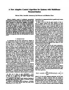
5 Simulation studies and results Simulations are carried out in Matlab to investigate the performance of the proposed ATSMC controller. A block diagram of ATSMC control scheme is shown in Figure 2. Based on the sampled input-output data of the servo system, the characteristic parameters are identified online by the RLS algorithm, which updating the parameters of the ATSMC controller. The PI controller is used for comparison. The system parameters used in simulations are listed in Table 1. To verify the adaptability to inertia variations, simulations are conducted in two cases, as shown in Table 2. To verify the robustness, a sinusoidal

(13)

where function  ( ) is defined as

1

0

s(k  1) s(k )   Ts(k )q p   T sgn  s(k )  d (k ) (20) Taking (16) into consideration, we have (21) d (k )   T sgn  s(k )     T

that



2

Then (19) can be written as

1 s(k )   Ts(k ) q p   T sgn  s(k ) (11) gˆ 0 ( k ) where  and  are positive constants, T is the sampling time, 0  q / p  1 is a ratio of odd integers, which guarantees that the sign of sliding function remains intact. Lemma 2 [9]. Consider the scalar dynamical system (12) z(k  1) z(k )  lz(k )  g (k ) where l  0 and 0    1 is a ratio of odd integers. If g (k )   ,   0 , there is a finite number k   0 such

1   1   1  ( ) 

(18)

  T sgn  s(k )   g 0 (k )u( k )

  Ts( k ) That is, s(k  1) s(k )   Ts(k ) q p   T sgn  s(k ) (19)  f (k ) x(k )  f (k ) x(k  1)  g (k )u(k ) q p

usw ( k ) 

1       z   ( )  max   , l1 (1 )  l     

1

 f 2 ( k ) x (k  1)  fˆ2 (k ) x (k  1)  s(k )

(14)

Define the lumped the identification error as

3

MATEC Web of Conferences 160, 05004 (2018) https://doi.org/10.1051/matecconf/201816005004 MATEC Web of Conferences EECR 2018

disturbance torque is added at 1.5s. The command position is a 60°step signal. fˆ1 ( k ), fˆ2 ( k ), gˆ 0 ( k ) 1z

r ( k ) 

ATSMC

u(k )

Online RLS identification

Servo system

parameters are fixed in case 1 and case 2 in order to investigate the adaptability and robustness. The position trajectories and tracking errors of the two controllers in case 1 and case 2 are shown in Figure 3 and Figure 4, respectively.

1z

1 z2

x(k )

Figure 2. Block diagram of ATSMC control scheme.

Figure 4. Position trajectories and tracking errors in case 2. Table 1. System parameters. Parameter

R L

Figure 3. Position trajectories and tracking errors in case 1.

After simulation adjustment, the parameters of PI controller are selected as k p  5.8 and ki  0.15 . The parameters of ATSMC controller are   0.5 , q  9 , p  13 ,   10 . The sampling time is T  0.005 . The RLS forgetting factor is f  0.995 . All of these

4

Value 1.3

Unit

kg m2 N  m/krpm kg m2

37.5

ke

67.2

kt

1.11

N  m/krpm

ks

3 10

N  m/rad

Jm

0.000323

kg m2

bm

0.015

N  m/krpm

JL

20.5/204.6

kg m2

6

MATEC Web of Conferences 160, 05004 (2018) https://doi.org/10.1051/matecconf/201816005004 EECR 2018 EECR 2018

bL

0.024

N  m/krpm

TL i

10

Nm

systems for its discrete-time form and easy implementation. For further improvement of tracking performance, the online identification method under circumstances of external disturbances are the future investigations.

178 Table 2. Two simulation cases.

Case 1 2

Load inertia 20.5 204.6

Inertia ratio 2:1 20:1

Acknowledgment This research was supported by National Natural Science Foundation of China under Grant No. 61333008, 61673217, 61673214, 61673219 and 61773211.

It can be observed from the simulation results that when load inertia varies from case 1 to case 2, the ATSMC controller keeps a good tracking performance with small overshot while PI controller produce a large overshoot in case 2. On the other hand, PI controller has larger steady-state error due to the disturbance torque. The ATSMC controller restrains the disturbance torque effect and the steady-state errors are smaller. This demonstrate that the ATSMC controller has better adaptability to inertia variations and stronger robustness to disturbances.

References 1. 2. 3. 4.

6 Conclusion In this paper, characteristic modeling method is extended to the servo systems with inertia variations. The characteristic model reduces the complexity of traditional mathematics model, and has more advantages in describing time-varying dynamics. Then, based on the characteristic model, a ATSMC controller is designed to improve robustness and achieve finite-time boundedness property. The adaptability and robustness of the proposed controller have been verified by simulations. The characteristic modeling method provides a feasible method of low-order controller design for complex systems. It is more practical in digital control

5. 6. 7. 8. 9.

5

Z. Li, C. Liu, F. Meng, K. Zhou, Proc. Inst. Mech. Eng. C 227, 1481 (2013) S. Li, Z. Liu, IEEE Trans. Ind. Electron. 56, 3050 (2009) S. Jee, J. Lee, Int. J. Precis. Eng. Manuf. 13, 1655 (2012) J. Jin, S. Wang, S. Huang, IEEE International Conference on Mechatronics and Automation (IEEE, Tianjin, 2014) J. Geng, Y. Sheng, X. Liu, Tans. Inst. Meas. Ctrl. 36, 604 (2014) L. Qi, S. Bao, H. Shi, Tans. Inst. Meas. Ctrl. 37, 875 (2015) Y. Xia, L. Dai, M. Fu, J. Frankl. Inst. 351, 2299 (2014) H. Wu, J. Hu, Y. Xie, Characteristic model-based intelligent adaptive control (China Science and Technology Press, Beijing, 2009) S. Li, H. Du, X. Yu, IEEE Trans. Auto. Ctrl. 59, 546 (2014)