Mar 12, 2006 - The training samples are a collection of input vectorsââx (produced by the ...... of some lesions in mammography (and also in chest radiography). ...... Mammography (DDSM) collected by the University of South Florida, and ...
Advanced Machine Learning Techniques for Digital Mammography
Matteo Roffilli
Technical Report UBLCS-2006-12 March 2006
Department of Computer Science University of Bologna Mura Anteo Zamboni 7 40127 Bologna (Italy)
The University of Bologna Department of Computer Science Research Technical Reports are available in PDF and gzipped PostScript formats via anonymous FTP from the area ftp.cs.unibo.it:/pub/TR/UBLCS or via WWW at URL http://www.cs.unibo.it/. Plain-text abstracts organized by year are available in the directory ABSTRACTS.
Recent Titles from the UBLCS Technical Report Series 2005-12 How to cheat BitTorrent and why nobody does, Hales, D., Patarin, S., May 2005. 2005-13 Choose Your Tribe! - Evolution at the Next Level in a Peer-to-Peer network, Hales, D., May 2005. 2005-14 Knowledge-Based Jobs and the Boundaries of Firms: Agent-based simulation of Firms Learning and Workforce Skill Set Dynamics, Mollona, E., Hales, D., June 2005. 2005-15 Tag-Based Cooperation in Peer-to-Peer Networks with Newscast, Marcozzi, A., Hales, D., Jesi, G., Arteconi, S., Babaoglu, O., June 2005. 2005-16 Atomic Commit and Negotiation in Service Oriented Computing, Bocchi, L., Ciancarini, P., Lucchi, R., June 2005. 2005-17 Efficient and Robust Fully Distributed Power Method with an Application to Link Analysis, Canright, G., Engo-Monsen, K., Jelasity, M., September 2005. 2005-18 On Computing the Topological Entropy of One-sided Cellular Automata, Di Lena, P., September 2005. 2005-19 A model for imperfect XML data based on Dempster-Shafer’s theory of evidence, Magnani, M., Montesi, D., September 2005. 2005-20 Friends for Free: Self-Organizing Artificial Social Networks for Trust and Cooperation, Hales, D., Arteconi, S., November 2005. 2005-21 Greedy Cheating Liars and the Fools Who Believe Them, Arteconi, S., Hales, D., December 2005. 2006-01 Lambda-Types on the Lambda-Calculus with Abbreviations: a Certified Specification, Guidi, F., January 2006. 2006-02 On the Quality-Based Evaluation and Selection of Grid Services (Ph.D. Thesis), Andreozzi, S., March 2006. 2006-03 Transactional Aspects in Coordination and Composition of Web Services (Ph.D. Thesis), Bocchi, L., March 2006. 2006-04 Semantic Frameworks for Implicit Computational Complexity (Ph.D. Thesis), Dal Lago, U., March 2006. 2006-05 Fault Tolerant Knowledge Level Inter-Agent Communication in Open Multi-Agent Systems (Ph.D. Thesis), Dragoni, N., March 2006. 2006-06 Middleware Services for Dynamic Clustering of Application Servers (Ph.D. Thesis), Lodi, G., March 2006. 2006-07 Meta Model Management for (Semi) Structured and Uncertain Models (Ph.D. Thesis), Magnani, M., March 2006. 2006-08 Towards Abstractions for Web Services Composition (Ph.D. Thesis), Mazzara, M., March 2006. 2006-09 Global Computing: an Analysis of Trust and Wireless Communications (Ph.D. Thesis), Mezzetti, N., March 2006. 2006-10 Fast and Fair Event Delivery in Large Scale Online Games over Heterogeneous Networks (Ph.D. Thesis), Palazzi, C. E., March 2006. 2006-11 Interoperability of Annotation Languages in Semantic Web Applications Design (Ph.D. Thesis), Presutti, V., March 2006.
Advanced Machine Learning Techniques for Digital Mammography Matteo Roffilli1
Technical Report UBLCS-2006-12 March 2006 Abstract A common thinking about the science is that every possible achievement can be pursued, provided that we have time and funds available for that purpose. On top of all this, recent technological achievements have carried this thinking to extremes, due to the speed of technological change sweeping through the world, which led to new momentous discoveries. Hence for researchers themselves there is every indication that by means of current technology they can be able to manage and solve every possible problem. Such a belief also took place in the late 1800s, when James Clerk Maxwell argued that what there was left to do in science was adding some decimals to the constants of the universe. Recent success in many branches of knowledge glutted the chance to propose new challenges which can stand for more than few years. For instance, the spread of Internet, the Human Genome Project, the conquest of Mars and the solution to the Fermat theorem are all cases worthy of mention. This delirium of omnipotence if, on the one hand, has been a source of complete satisfaction and proudness, unleashed on the other hand what can be called the ancestral human fear of unknown. Common people experience a sort of “horror vacui”, they feel threatened by something they are afraid to lose control of. If the science produces knowledge, technology, which is the application of science, can turn out to be an innovation available to the most part of the people, thus causing welfare of the society, or only to the few, consequently becoming an instrument of power. And what is more, the current discoveries make people forecast puzzling employments, which are far more exceeding than the time travels opened up by the relativity theory. This supports the common belief that technological applications, which we will henceforth name machines, can neither be superior to, nor emulate the primary human faculty, namely the thought. It is thus a common thought that machines are stunning but stunted tools and nothing more. In 1950 Alan Turing pronounced against this belief, claiming that it would have been possible to build a machine which could be able to face human being on the field of thought itself. This intuition initiated the project of Artificial Intelligence and the study of technology which might make the machines capable to acquire knowledge autonomously, instead of being programmed by a human being for that purpose. Machine Learning is the specific topic which this thesis deals with. Recent developments in Statistical Learning Theory led to the first appearance of powerful algorithms of automatic learning which face the problem from a statistical point of view. The forefather of this set of algorithms is Support Vector Machine (SVM), which was put before the research community for the first time on occasion of the Conference COLT 1992 and which soon afterwards has been considered one of the most promising instruments for Machine Learning. Against this backdrop, this thesis aims to demonstrate that advanced technologies of Machine Learning based on SVM can effectively solve complex problems, which cannot be currently faced by traditional 1. Department of Computer Science, University of Bologna, Mura A. Zamboni 7, 40127 Bologna, Italy.
1
research technologies. The problem chosen for this work is the diagnosis of breast tumour through digital mammography. The reason for this choice lies in the fact that this problem is regarded as one of the hardest to solve on the field of objects recognition. The difficulty about carrying out researches into complex images lies not only in the process itself, since even the radiologists find it tough to identify lesions, given their great variability in shape, dimension and appearance. Moreover the creation of a Computer Aided Detection system would provide for a huge benefit in the hospital field, which is constantly looking for expert radiologists, and would have sensible effects on medical and ethical ground. Our aim is to make some contribution to the demonstration of the applicability of Machine Learning technologies to the diagnostic problem. This thesis specifically proposes a cancer detection system which is capable to find lesions not by means of an algorithm based on prearranged features, but by analogy with other previously analised lesions. In other words, the system is trained to recognize different typologies of lesions which are present on a dataset prepared for the purpose. The system can also find autonomously lesions with similar characteristics in unknown mammographies. This innovative achievement is made possible by the use of SVM as classifier for a typological classification. In order to maximize the potential of SVM, a new detection system has been developed so that the image is classified without an object detection phase. In other words, this new method differs from the past ones, since it is no longer necessary to extract objects and their characteristics before the classification. The ultimate achievement of the set system consists in superimposing some markers upon an unknown mammogram. The markers identify zones where we have high probability to detect a tumoral lesion. This thesis submit our reports on the effectiveness of the method by means of tests which compare our new achievements with the state of the art in imaging method, both on standard dataset, and on images acquired by partner hospitals for this purpose. The startling originality of the method proposed is confirmed by the fact that a few national and international patents have been taken out on it.
UBLCS-2006-12
2
Dedicated with love to my family, my grandparents, my parents and Annica who have made it possible.
UBLCS-2006-12
3
Chapter 1
Introduction The quest for the truth led science right from the start. At the beginning the research on the one hand directed its attention to the great ontological questions, on the other hand it was driven by the fulfillment of basic needs. The hazy border line between the two questions was not distinguishable, to the extent that similar methods were applied and the same persons used to tackle both challenges with great aplomb. The first and still unmodified distinction between the two branches is due to Galileo Galilei, whose method relied to the principle according to which sciences ought to carry out experiments and justify them through mathematical demonstrations. This principle is nowadays still generally spread and regarded as valid among scientists, affecting the research method on the most disparate fields of knowledge. These preliminar observations on the method must always be kept in mind if we wish to avoid falling into temptation of a simplicistic logic, which might lead to hasty conclusions. Obviously, at this regard some fields are more exposed than others. It would commonly seem much easier to draw a rash inference in social or economical analyses than in mathematical or physical ones. Therefore when the study of intellective skills is involved, the complicacy of the topic strengthens the belief that human brain is too a complex subject for drawing certain and provable conclusion on it. Artificial Intelligence (AI) is a symptomatic case of the above-mentioned dynamics. It is thanks to researches and ideas of Alan Turing that this new branch was born in 1950s. Afterwards it quickly passed through the different phases we cited above. Originally, the motivation was really pretentious: matching human brains abilities in complex situations. Notwithstanding the initial promising discoveries, it was soon evident that this achievement was hardly attainable in a short time. Nevertheless, the fresh impetus and the aroused expectations supported the researches also during the dark times sparkling with the progressive collapse of expectations. Among the developed methods, the study on Artificial Neural Networks (ANN) arose, and still nowadays keeps on arising, great interest. The analogies which this system boasted with biological systems, analogies which it still claims, gave new impulse to this sector up until the famous article by Papert & Minsky, that raised a serious question about the real capacities of the first ANN: the Rosenblatt perceptron. Fortunately, the hurdle has been cleared and the ANN are of high repute as effective systems for the resolutions of real problems. In spite of their wide diffusion, neural networks have no longer a deepened theoretical justification. The reason probably lies in the fact that they are born on an experimental basis (the so called heuristic method) and only subsequently it has been tried to find an acceptable reason for their smooth functioning. Another example of such a phenomenon is adaboost algorithm, which is widely spread in order to train classifiers. Using a fashionable expression in Computer Science, we may say that ANN are not Galileocompliant, in the sense that they do not fully follow the Galilean paradigm. They have in fact an immense number of case studies on the field of the sensible experiences, but they lack of necessary demonstrations. Following a complementary path, over the last ten years a new method for the creation of Machine Learning came into the limelight. Such a method, called Support Vector Machine, is born as a direct implementation of a learning theory based on statistical framework. Statistical Learning Theory (SLT) began to develop early on in the sixties by two Russian math4
1
Motivation and goals
ematicians named V. Vapnik and V. Chervonenkis. For about thirty years these two researchers have been looking for a new principle capable of overcoming a few drawbacks that the moment theory involved. In particular, they proposed a new learning principle which could lead machines throughout their learning process, namely the Structural Risk Minimization (SRM). As this thesis aims to show, by SRM the machine is forced not only to try to learn an experience at disposal (namely the Empirical Risk Minimization ERM), thus maximizing its potential, but it is also compelled to develop a model of knowledge of right complexity which is able to answer properly even in new situations (in other words, it must be able to generalize). All SLT it is a rigorous and formal demonstration that it is possible to take advantage of this concept in order to build machines capable of an effective learning in difficult contexts. In 1992 this theory was formalized with an algorithm, namely SVM, and was submitted to the scientific community. From that moment on SVM gained an enormous popularity. Currently it is really difficult to find out some scientific field on which SVM (and SLT) is not successfully applied. Several control experiments confirmed the excellence of SLT, thus supporting Vapniks claim: “Nothing it is more practical than a good theory”. In this respect SLT and SVM keep strictly to Galilean paradigm.
1
Motivation and goals
Against this backdrop, this thesis aims to demonstrate that advanced technologies of Machine Learning based on SVM can effectively solve complex problems, which cannot be currently faced by traditional research technologies. The problem chosen for this work is the diagnosis of breast tumour through digital mammography. The reason for this choice lies in the fact that this problem is regarded as one of the hardest to solve on the field of recognition of objects into images. The difficulty about carrying out researches into complex images lies not only in the process itself, since even the radiologists find it tough to identify lesions, given their great variability in shape, dimension and appearance. Moreover the creation of a Computer Aided Detection (CAD) would provide a huge benefit in the hospital field, which is constantly looking for expert radiologists, and would have sensible effects on medical and ethical ground.
2
Novel contributions
Our aim is to make some contribution to the demonstration of the applicability of Machine Learning technologies to the diagnostic problem. This thesis specifically proposes a cancer detection system which is capable to find lesions not by means of an algorithm based on prearranged features, but by analogy with other previously analised lesions. In other words, the system is trained to recognize different typologies of lesions which are present on a dataset prepared for the purpose. The system can also find autonomously lesions with similar characteristics in unknown mammographies. In particular, the novel contributions of this work are mainly three: 1. the detection step is performed without the use of external knowledge (e.g. threshold value, appearance model, etc.) relying only on preexistent data; 2. the feature extraction step is avoided: all the information available on the mammogram is exploited; 3. SVM is used as classifier for the classification step. As it will be afterwards clarified, the three contributions are strictly joined since each one necessarily depends on the others. The ultimate achievement of the set system consists in superimposing some markers upon an unknown mammography. The markers identify zones where we have high probability to detect a tumoral lesion. This thesis submit our reports on the effectiveness of the method by means of
UBLCS-2006-12
5
3 Thesis organization
tests which compare our new achievements with the state of the art in imaging method, both on dataset, and on images acquired by partner hospitals for this purpose. As a corollary to this result, advanced optimization techniques have been developed and implemented with a view to dealing with the computational problem by means of common personal computers.
3
Thesis organization
This thesis is organized as follows. The first part introduces the statistical learning framework and the Support Vector Machines. The second part present the application of such machine learning techniques to the problem of cancer detection. Chapter 2 presents the learning paradigm and its statistical interpretation. It introduces the notion of learning and specifically learning from data. Chapter 3 contains the basic ideas laying behind the Statistical Learning Theory, trying to give an useful insight into the work, which provides for an overall understanding. Chapter 4 illustrates a qualitative overview on Support Vector Machine for classification, regression and innovative detection, while the mathematical details are discussed in Chapter 5. Chapter 6 makes a review of new promising learning algorithms inspired to the SVM. Chapter 7 reviews the optimization framework for efficient training of a SVM and common software package available by the research community for this purpose. The Chapter further proposes a novel implementation of the testing phase of SVM that makes use of DSP technology. Chapter 8 presents a general view of the mammographic field providing the basic knowledge about medical imaging. Chapter 9 discuss the state of the art of current system for aided detection, while Chapter 10 is a survey of the application of SVM to digital mammography. Chapter 11 presents common methods for data representation. Chapter 12 presents in detail the novel contributions of this work. Chapter 13 reports and summarizes results obtained in several experiments we conducted in order to demonstrate the viability and the efficiency of our approach. Chapter 14 concludes the thesis by summarizing the obtained results achieved and by outlining future plans of research.
UBLCS-2006-12
6
Part I Theoretical foundation
UBLCS-2006-12
7
Chapter 2
Learning Paradigm 1
Introduction
The problem of learning has been investigated by philosophers throughout history, under the name of inductive inference. Although this might seem surprising today, it was not until the 20th century that pure induction was recognized as impossible unless one assumes some prior knowledge. This conceptual achievement is essentially due to the fundamental work of Karl Popper [115] (based on Hume’s ideas [63]). The main idea of the Machine Learning is that it is possible to gain knowledge starting from experience or data (i.e. a collection of objects) without understanding the internal mechanism that has generated such data. Knowledge gained through learning partly consists of descriptions of what we have already observed, and is partly obtained by making inferences from (past) data in order to predict (future) outcomes. This second part is usually called generalization, or induction. Obviously if data have no regularities, in the sense that it does not possess any law as a part of themselves, we won’t be able to find any new knowledge. The main aim of this process is to make some predictions about future objects, to make some decisions or just simply to understand. Indeed, the field of Machine Learning has been greatly influenced by other disciplines and the subject is in itself not a very homogeneous discipline but includes separate, overlapping subfields [38]. The technical realization of artificial Machine Learning devices may thereby have economic and social advantages. The design of such systems demands scientific knowledge of the human pattern recognition ability. Moreover, the realization and evaluation of the use of such systems may further increase this knowledge. The above-cited process suggests that a distinction can be made between the scientific study of Machine Learning as the ability to generalize from observations and the applied technical area of the design of artificial Machine Learning devices, without neglecting the fact that each one may highly profit from the other. The task of building learning machines can be tackled inside different conceptual frameworks. The choice is mainly driven by the goals to attain and also by the scientific background of the pratictioner. Historically, there was a great debate on what approach is the best but no ultimate answer has been found. Currently, the statistical framework is becoming the most promising approach to Machine Learning. It is grounded on a well-founded analytical theory and it is demonstrating superior performance on standard test problems.
2
Statistical formulation
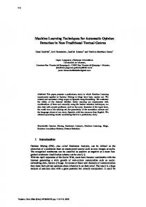
The statistical setting of the learning task involves three components: → 1. a generator of input vectors − x 8
2 Statistical formulation
SYSTEM
x
P( y|x)
y LOSS FUNCTION
y
GENERATOR
P( x)
L(y,f(x)
x
LEARNING MACHINE
f (x)
f
Figure 1. The statistical framework.
→ 2. a system (under analysis) which returns an output y in response to a given vector − x 3. the learning machine f (e.g. a function or an algorithm) which learns (estimates) the unknow dependency between the generator and the system. → The generator produces current and future (yet not observed) input vectors − x drawing them i.i.d. (independently and identically distributed) from some unknow probability density → p (− x)
(1)
that does not change during time (i.e. it is stationary). Indeed, the theory derives analytically important results by exploiting the assumption that the probability density does not change with time. If this happens, the validity of all theoretical results is lost. However, while the assumption is quite strong, it can be considered as true for many common problems. → The system f produces an output value y for every input vector − x according to some conditional density → p (y|− x) (2) that is unknow. The conditional density models, from a statistical perspective, the internal mechanisms of the system as a whole. The system’s behavior is considered as a black box: the main goal is to capture what the system does and not how it works. The learning machine is a mechanism (an algorithm) able to choose a particular function from a set of available functions that approximate the system’s behavior at the best. According to the black box intuition, the learning machine estimates the mapping function that associates a → particular output y to a given input − x but it does not explain the dynamics of the mapping. A key consideration is that the mapping is considered fixed (stationary) for all the inputoutput couples. Roughly speaking, it means that the mapping function does not depend on time. For these simple reason, it is clear that finding temporal dependencies among data is a difficult task inside the statistical framework. The first aroused issue is about how we can measure the performance of a learning machine. To this aim, the following error measure, called the loss, is introduced: → L (y, f (− x ))
(3)
The loss L measures the discrepancy between the output y produced by the system and the → output of learning machine f at a given point − x . The expected value of the loss R, called expected risk, is defined by means of the following risk functional: UBLCS-2006-12
9
2 Statistical formulation
� R=
→ → → → L (y, f (− x )) p (y|− x ) p (− x ) d− x dy
(4)
It is worth noting that the expected risk corresponds to the sum of the loss computed over → all possible input parameters − x . This way the expected risk quantifies how good is the learning machine in totu. The loss and the expected risk are key points since every result is expressed exploiting these concepts. Whatever the loss, the machine learning process is subdivided in two stages: 1. learning (or parameter estimation, parameter fitting, model fitting) from training samples; 2. prediction for test samples. → The training samples are a collection of input vectors − x (produced by the generator) that are used to learn (to estimate) the unknow dependency. The test samples are a collection of input → vectors − x (drawn i.i.d. from the same fixed distribution) for which the trained learning machine predicts the output value. According to this setting, three major tasks can be solved: 1. classification; 2. regression; 3. density estimation (also referred as clustering, partitioning or vector quantization). There is an alternative distinction between supervised and unsupervised learning problem. In the supervised setting, for each train samples the system’s output y is available as a real value or as a label. In this view, the system is considered as a supervisor external to the generator. Classification and regression fall into this group. In the unsupervised setting the system is not available and thus no output are associated with input. Density estimation falls into this group. 2.1 Classification In the classification task, the available data consists of pairs of input objects and corresponding labels given by the system. The task of the classifier (i.e. the learning machine that performs the classification) is to learn (estimate) the mapping function. A classification task with only two class is named binary classification (or dichotomic classification). In this case the mapping function belongs to the class of indicator functions. If the classes are more than two we are dealing with a multiclass classification task. The loss associated with the classification task is: � → 0 if y = f (− x) → − L (y, f ( x )) = → 1 if y �= f (− x) 2.2
Regression
The regression task is equivalent to the classification except for the fact that the system’s output is a continuous value. One possible loss function is: 2 → → L (y, f (− x )) = (y − f (− x ))
(5)
A typical regression problem is the well-known fitting problem. In this case the learning machine has to choose a fitting function and then it has to estimate the parameters that minimize the risk functional associated with the loss. 2.3
Density estimation
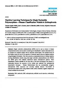
The density estimation task takes account of problems in which the system’s output is unknow or not available (see Figure 2). → In this case, the goal of the learning machine is to find a probability density function p (− x) that captures the behavior of the generator. While density estimation is often presented as an UBLCS-2006-12
10
;; ;;
3 Learning process
SYSTEM
P( y|x)
GENERATOR
P( x)
x
LEARNING MACHINE
LOSS FUNCTION
L(x, f(x)
f (x
)
f
Figure 2. The statistical framework for density estimation.
extension of classification/regression, indeed it is the main problem because it estimates the pdf needed to compute the functional risk 4. A classical loss function for this problem is: → → L (y, f (− x )) = − ln (− x)
(6)
While in the supervised setting the learning machine is able to compute a meaningful error measure, in the unsupervised setting there is not a clear way to assess the goodness of the learning. This well-known issue is very common in the clustering setting. In this case, the goal is to find a partition of the objects produced by the generator. Similar objects should belong to the same partition while different objects should belong to different partitions. The most challenging problem is to define a priori the number of partitions. Then the membership to the prefixed partitions can be easily achieved defining ad hoc loss functions. For instance, considering a bimodal distribution, it can be shown that the optimal number of partition is two. Given this a priori knowledge, a learning machine can efficiently find the membership function measuring the distance of each object from the centers of the two partitions and then choose the closest one.
3
Learning process
As reported by [47], the problem of learning can be divided in two parts: 1. specification; 2. estimation. Specification consists in determining the type of functions (or models) that will be used in the learning task. Estimation determines (or estimates) the operative parameters of the functions from the data available. Secondly, we must also decide the learning principle, which lies at the heart of a learning algorithm. The learning principle, called inductive principle, is a general prescription that declares what to do with the data, i.e. what is the result to obtain. The learning method (or algorithm) is a constructive implementation of the inductive principle and tells us how to obtain the result.
UBLCS-2006-12
11
4 Inductive principle
4
Inductive principle
The most intuitive inductive principle starts from the idea that minimizing the empirical risk, i.e. the discrepancy between the estimated function and the true function, in the available points of the input space (i.e. the samples) is a good way to find the best approximator of the system. This principle is called Empirical Risk Minimization (EMR) inductive principle. Being a general principle, the ERM does not need demonstration. Nevertheless, when using the ERM there are two important proprieties to be discussed: 1. if it is consistent: if the empirical risk will converge toward the expected risk; 2. what is the learning rate: how fast will it converge. Another important issue regards the size of the training set. Many theoretical results are justified asymptotically in the light of the Laws of Large Numbers. In practical problems the number of available samples is often very low and hence analytical results can not be applied straightforward. The next chapter addresses all these issues.
UBLCS-2006-12
12
Chapter 3
Statistical Learning Theory in a nutshell The Statistical Learning Theory (SLT) is a theory developed by Vapnik and Chervonenkis [157] in order to analyze the learning process from a statistical point of view. Roughly speaking, SLT is a conceptual framework able to analytically (mathematically) formalize the learning process and to manage the relative issues by means of statistical methodologies. A fully presentation of the framework is outside the scope of this section. For an overall description see [32], [73], [126] and [158]. The goal of this section is to sketch some fundamentals ideas useful for understand the construction of new well-founded learning algorithms. As stated in the previous chapter the problem of predictive learning can be summarized as follows: 1. given past data and reasonable assumptions; 2. estimate unknown dependency for future predictions. The SLT refers to the term reasonable assumptions and involves mathematical, statistical, philosophical, computational and methodological issues. Contrary to other learning theory, SLT makes a clear separation among: • problem statement; • solution approach (i.e. the inductive principle); • constructive implementation (i.e. the learning algorithm). SLT is composed by four main blocks: • condition for the consistency of the ERM inductive principle; • VC-dimension and formulation of bounds on the generalization ability; • new inductive principle for small samples: Structural Risk Minimization (SRM); • methodology for implementing the SRM.
1
Consistency
The starting point is the consideration that current learning theories move from the idea of asymptotic error. The measure of goodness of a learned model (i.e. expected risk), is performed for all the possible input variables. Unfortunately, the expected risk can not be evaluated because of the fact that the probability distribution of input variables is unknow. On the other hand, we can measure the error on the training data available (i.e. empirical risk). Stated that the expected 13
2 VC-dimension
risk can not be measured, using the empirical risk to measure indirectly the performance of the learned model seems to be a reasonable assumption. As presented before, the goal of the Empirical Risk Minimization inductive principle is to minimize the empirical risk in order to indirectly minimize the expected risk and so to achieve overall good performance. Minimizing the empirical risk is not a bad thing to do, provided that sufficient training data n is available, since the Law of Large Numbers ensures that the empirical risk will asymptotically converge on the expected risk for n → ∞ This general property of an inductive principle is called (asymptotic) consistency. The contribution of the SLT is the demonstration that the ERM inductive principle is consistent for every approximating function (that uses this principle) if and only if the empirical risk converges uniformly on the true risk in the sense presented in [159]. In other words, the analysis of consistency is driven by the worse function that can be chosen from the set of functions implementing the ERM, i.e. the function that produces the largest discrepancy between the empirical risk and the true risk. This conceptual achievement stresses the point that each analysis of the ERM is a worst-case analysis.
2
VC-dimension
In order to be as general as possible, it is a good request that a theory does not depend on particular distribution of samples (in this case the bound is termed distribution-dependent). To this aim, SLT introduces an analytical measure of the complexity of a model (i.e. a learning machine) that is independent from a particular distribution. This measure, called VC-dimension, numerically quantifies the complexity of a set of functions implemented in a learning machine. Following [32] we adopt a constructive (an more simple) definition of VC-dimension based on the notion of shattering: if n samples can be separated by a set of indicator functions in all 2n possible ways, then this set of samples is said to be shattered by the set of functions. Thus a set of function has VC-dimension h if h samples exist that can be shattered by this set of functions but h+1 sample that can be shattered do not exist. In other words, given a set of functions, if it is possible to find at least one configuration of n points that can be binary labeled in all ways by this set of functions, then its VC-dimension is n (i.e. h = n). It is worth noting that VC-dimension is a property inherent in a set of functions and does not depend on a particular distribution of samples. Using this result, it becomes possible to formulate the consistency of the ERM inductive principle in a distribution-independent way. However, for small samples, one cannot guarantee that ERM will also minimize the expected risk.
3
Rate of convergence
In order to develop a learning theory valid for small samples size, it is of main interest to estimate how fast the empirical risk converges on the expected risk. Recalling that the degree of speed is relative to the number of samples, the main measure of convergence is the discrepancy between the empirical and true risk as a function of the number of samples or the upper bound of this measure that can be derived more easily. In computing the bound we must evaluate is the loss function chosen for the specific task. SLT provides many useful bounds for different loss functions. For classification task the bound can be presented as: � � n − ln η (1) R (ω) ≤ Remp (ω) + Φ Remp (ω) , , h h where ω is a general learning machine, n is the number of samples, h is the VC-dimension and η is the confidence level for which the bound holds. Technical considerations apart (see [32]), the bound states that the risk of error of a learning machine is equal or lesser than the empirical risk plus a second term, called confidence interval, that primarily depends on the ratio between the VC-dimension and the sample size (keeping fixed other parameters). If the ratio nh is large UBLCS-2006-12
14
error
4 Structural Risk Minimization
bound on test error
R
confidence level
training error
R emp h
structure S k -1
Sk
S k +1
Figure 1. SRM principle: according to formula 1 SRM choses (arrow) the machine with the best bound on test error
the confidence interval decreases (to zero) and the empirical risk can be used as a measure of the true risk. In this case the ERM principle is justified. If the ratio nh is small the confidence interval starts increasing. In this case the ERM principle loses its validity and another principle has to be used.
4
Structural Risk Minimization
From the bounds 1 it is evident that the true risk can be approximated only controlling both the empirical risk and the confidence interval. While the first depends on a particular set of samples (and the particular function chosen to minimize the loss), the second depends only on the class of function (and the relative VC-dimension). In order to minimize the true risk, a learning machine must controll both terms. Hence the VC-dimension must become a controlling variable during the learning phase. During the minimization the learning machine has to find the class of functions having optimal VC-dimension for the given set of samples and then to estimate the best function (minimal empirical risk) available in such class. The Structural Risk Minimization (SRM) inductive principle provides a formal mechanism for choosing an optimal model complexity (VC-dimension) for a finite set of samples. The main idea of SRM is that the approximating functions are arranged in a nested structure in which each subset includes the smaller one and every subset has a finite VC-dimension. S1 ⊂ S2 ⊂ . . . ⊂ Sk ⊂ . . .
(2)
By moving from a subset to a smaller one, the learning machine implicitly controls (reduces) the VC-dimension and then, according to 1, the true risk. h1 ≤ h2 ≤ . . . ≤ hk ≤ . . .
(3)
From a constructive point of view, the SRM can be implemented as follows: UBLCS-2006-12
15
4 Structural Risk Minimization
1. For a given set of samples, select from the set Sk the function fk (x) that minimizes the empirical risk. For instance: select the w0 and w1 parameters from the set of polynomial functions of degree 1: f (x) = w0 + w1 x. 2. Then the guaranteed risk of the function is found analytically exploiting the bound 1. 3. Compute the guaranteed risk for every subset (i.e. tries polynomial functions of different degree). 4. Choose the function that has the best (low) guaranteed risk. It is worth noting that the SRM does not specify a particular structure. Each particular choice of a structure gives raise to a different learning algorithm, consisting of performing SRM in the given structure of set of functions. The structure at the basis of the Support Vector learning algorithm is the set of separating hyperplanes.
UBLCS-2006-12
16
Chapter 4
Support Vector Machines: a qualitative approach The SLT previously presented gives some useful bounds on the generalization capacity of a learning machines that follows the SRM principles. However, SLT does not specify how to build such a machine. The first attempt to create a learning machine based on the SLT, also known as VapnikChervonenkis theory [158], was the Support Vector Machine (SVM) algorithm.
1
Brief history
The Support Vector Machine was invented by Vladimir Vapnik and his colleagues at AT&T Bell Laboratories and first introduced in 1992 at the Computational Learning Theory (COLT) conference. The roots of this approach, the Support Vectors method of constructing the optimal separating hyperplane for pattern classification, go back to 1964 work by Vapnik and Chervonenkis. In 1992 the SV technique was generalized for nonlinear separating surfaces by Boser, Guyon and Vapnik. In 1993-95 it was extended for constructing decision rules in the non-separable case (the soft margin version) by Cortes and Vapnik [35]. In 1995 the SV method for estimating realvalued functions (regression) was obtained by Vapnik and in 1996 the SV method was adopted for solving linear operator equations by Vapnik, Golowich and Smola. Further, in 1999 the SV method was applied to solve density estimation problems. Nowadays, SVM has become one of the standard tools in the Machine Learning community for classification, regression and density estimation tasks.
2
Binary classification
The binary classification context imposes to deal with objects belonging to two different classes: the “positive” and the “negative”. There is no special motivation to label one class as positive except when we are interested in searching particular target objects surrounded by others. In this case, the target objects are called positives. The problem of finding a way to separate positive objects from negative ones is called learning. During the learning phase the algorithm chosen for the search needs to know the exact label of each object under analysis. For this reason, such problem is named supervised learning, stressing the point that an external supervisor must provide the labels. After the learning is finished, the algorithm is able to apply the learnt way to unseen and unlabeled objects in order to predict their label. Both algebraic and geometric approaches can fully describe how SVM performs the supervised learning task. In the present survey, we adopt the geometric approach. In principle, there are no limitations on the kinds of objects under analysis. They can be, for example, measures, molecules, sounds or images. In every case, in order to enable the learning algorithm, running on a computing machinery, to deal with those objects the analyst must 17
2
Binary classification
Feature 2
Input space
Feature 1 Figure 1. A input space with two features: triangles are objects of class “positive” and squares of class “negative”.
obtain a numerical representation of them. This step, i.e. the issue of data representation, may seem obvious but it is responsible for the main effort to develop classifiers for real-world problems. In Chapter 12 a promising technique to overcome this issue will be presented. In a general framework, it is possible to represent an object by means of a collection of real-valued characteristics that exploit particular properties of interest. In this case, each object behaves as a point in an n-dimensional space, where n is the number of characteristics collected, called features. This special space is named input space (see Figure 1). If the input space allows the definition of a distance measure between the objects inside, the space is said to have a metric. Indeed, a learning algorithm exploits the distance measures between two objects interpreting that as a similarity measure. The key idea behind this measure is that objects of the same class should be close in the input space and consequently their distance measure should be small. In essence, the following is an explanation of how an algorithm can be designed to exploit this similarity measure, in order to separate objects of different classes. From this, it is clear that if the data representation does not provide an input space with a powerful discriminating measure of similarity, there is no way to achieve good classification results. A bunch of algorithms has been developed to solve the separation task. The main difference among them resides on which kind of discriminant function should be used and on how it can be estimated. The most important divergence is between linear and nonlinear functions. A linear function can be easily estimated, but often it is not flexible enough to separate correctly the objects, when the problem is intrinsically nonlinear. In this case, the learning algorithm must explore the more powerful class of nonlinear functions. Indeed, the main risk in this proceeding lies in the fact that flexible functions can approximate the bounds of the objects too well, loosing generalization ability. This well-known dilemma is named overfitting. A widely used strategy to tackle this problem relies on the concept of smoothness. The smoothness, or capacity value, quantifies how much a function (or a class of functions) is complex. It is widely accepted that smoother the function is, better will be its generalization ability. Exploiting this knowledge, the learning algorithm tries to find the discriminant function that both makes fewer errors and is less complex. In particular, SVM manages the trade-off between learning errors, called empirical risk, and function complexity, called VC dimension, implementing a hybrid strategy. In the following survey, an intuitive explanation of the SVM method is presented. For a detailed description of the mathematics behind SVM, see Section 5. UBLCS-2006-12
18
2
Input space
Feature 2
Feature 2
Input space
Binary classification
Feature 1
Feature 1
Figure 2. Two admissible linear classifiers with their distance from nearest objects (shaded in gray) and an unknown object (circle).
A set of objects S is called a linearly separable set, if it is possible to find in the input space a hyperplane from which the distance of all objects of the positive class is greater than zero, and of the negative class is lesser than zero. It is worth pointing out that the hyperplane is provided with a direction. In this way, it becomes possible to define a right and a left side of the hyperplane, or analogously a positive and a negative side. The aim of the learning algorithm is to place the hyperplane in such way that all positive objects will be placed on the positive → side and all negative objects on the negative one. Then, given an unknown object − x and the separating hyperplane, it is possible to define the class it belongs to by checking on what side of the hyperplane the object is. It is easy to check out that a linearly separable data set allows an infinite number of separating hyperplanes. The key question is which the best hyperplane to choose is. To tackle this issue, it is necessary to introduce the first key idea of SVM: the margin. When a hyperplane is applied to a set of objects, an important measure can be computed: the minimum distance of the hyperplane from the closest object. This value, called margin, measures how much the hyperplane can be moved without affecting the separation. From the object perspective, the margin predicts how much it can be moved without changing the belonging class. It is worth noting that larger margin guarantees that the classification is more robust to perturbation. Figure 2 shows two admissible linear classifiers with their margin and an unknown object. Relying on this idea, SVM finds the hyperplane with margin maximal respect to the dataset. From this reason, SVM is named a maximal margin classifier. The objects at minimal distance from the hyperplane are called Support Vectors, because they are supports for the definition of maximal margin hyperplane. Indeed, the name “Support Vector Machine” derives from this fact. From a mathematical point of view, the quest for SV is formulated as a Quadratic Programming (QP) problem with convex constraints. The solution relies on the optimization theory and its relative techniques. In particular, the exploitation of the Lagrangian theory, developed in 1797 for mechanical problems, introduces the second key idea of SVM: the duality. The duality, or the dual representation, is an alternative way to formalize and to solve the QP problem. By exploiting particular properties of the formulation in the dual representation the size of the problem is bound to the number of samples and not to the number of features like as in the original (primal) formulation. Apart from mathematical details, the main advantage is that many off-the-shelf efficient algorithms can solve efficiently this kind of problems. In addition, the duality opens the way to solve efficiently the separation task in the case of nonlinear separable data. In the nonlinear case, the relative QP problem cannot be solved because some constraints cannot be satisfied. In order to make it possible, the SVM exploits a third key idea: an efficient learning algorithm should be able to make errors. Formally, this result is achieved adding penalty UBLCS-2006-12
19
2
Binary classification
Feature 2
Input space
slack
margin margin
Feature 1 Figure 3. Soft margin, slack variables and Support Vectors (circled).
variables, called slack variables, to the problem constraints. The value of the slack variables becomes greater than one only when the associated object is placed on the wrong side. Hence, the number of variables with value greater than one bounds the maximal number of errors. The margin defined by the hyperplane with slack variables is said to be a soft margin, stressing that the learning algorithm is dealing with a nonlinear separable dataset. Figure 3 shows an example of soft margin, separating two classes non separable in a linear way. Here, the slack variable becomes greater than one for the square located on the wrong side (among the triangles). It is well known that SVM finds a linear separating hyperplane as other methods do. According to the Statistical Learning Theory, i.e. the theoretical foundation of SVM, the maximal margin hyperplane reaches a negotiation between the separation errors (fixed to zero in the linerly separable case) and the complexity of the discriminant function (i.e. the confidence interval of making errors in the future). In addition, SVM performs the flexible management of outliers, by means of the soft margin mechanism. While the soft margin can be helpful in increasing learning robustness, the class of linear classifiers seems to be inadequate to tackle many real-world applications. Objects represented by high-dimensional features need a more powerful class of classifiers, able to produce nonlinear decision boundaries. To this aim, two main strategies can be deployed: • the complexity of the classifier can be increased working on the architecture and the training procedure: historically, this approach developed the multilayer perceptron starting from the perceptron; • the complexity of the data representation can be increased: performing a linear separation in a nonlinear space intuitively is similar to perform a nonlinear separation in a linear space. Each of the two ways has some advantages and some disadvantages. Through the first approach, a more complex architecture could have many degrees of freedom, and consequently a large number of parameters. As a result, training such classifier is quite complicated: a large number of parameters have to be estimated using a limited number of samples. This is the wellknown issue named curse of dimensionality. On the contrary, the data representation has not to be modified and can be directly used by the algorithm. Through the second approach, the designer must choose a fixed mapping, combining original features in nonlinear manner, and then the linear algorithm can be used. The idea is the followUBLCS-2006-12
20
3
Feature space
mapping
Feature 1
Feature 2
Feature 2
Input space
One class classification
Feature 1
Figure 4. A nonlinear mapping function maps the data from the input space to the feature space.
ing: to define a nonlinear mapping function of the original input space into a new space, called feature space, and then to move objects to the new space according to the mapping (see for instance Figure 4). When a similarity measure between two objects is needed, the algorithm computes it in the feature space. While this procedure perfectly works, the computational effort may be unaffordable since the feature space usually has a dimension higher than the original one, resulting in a computational effort extremely high. Another approach based on a radically different perspective has been developed: the kernel method. The main idea relies on the fact that SVM does not need exactly to know the values of all the features of each object. What it really requires is the similarity measure of each couple of objects. Indeed, in the dual form of the QP optimization problem the measure of distance (similarity) between objects is present only in a compact form called scalar product. If there is a way to directly compute the value of this quantity in the remapped space, it could be possible to bind the computational cost. A mathematical trick, called kernel, can be exploited for this aim. Intuitively, a kernel is a measure of similarity between two vectors in a remapped space. When the vectors are similar, their kernel value is “large”, when they are not similar their kernel value is “small”. Interestingly, the kernel function directly computes the distance measure without the explicit remapping. Thus, it results computationally feasible. Hypothetically, one can predefine the distance measure of each couple of objects, and then use it as a kernel function. Another useful property of the kernel function is that it is independent from the dimension of the input space. According to this behavior, SVM is said to be a dimension free classifier. Avoiding the explicitly remapping of each feature, the kernel function can manage vectors of huge dimension at virtually no additional cost. Exploiting the kernel function, every linear algorithm based on the scalar product can be transformed into a nonlinear one, by substituting the scalar product with an appropriate kernel. This procedure is named kernelization [127]. Obviously, some mathematical details must be taken into account, but the kernelization procedure is quite easy. Using this trick, it becomes possible to design nonlinear SVMs without modifying the algorithm. Obviously, the choice of a particular kernel is a design parameter. There is a lot of work in making better kernels, in order to embed a priori knowledge of the problem in the machine. The use of kernels is becoming a separated research area of Machine Learning to the extent that the SVM and a bunch of classical algorithms extended with kernel function found the field of Kernel Machines.
3
One class classification
Let’s imagine now that the labels of the objects are not provided. In this case the framework of binary classification can not be applied since we do not have two classes to separate but only one class. Indeed, this special kind of problem is called one-class classification or alternatively novelty UBLCS-2006-12
21
3
Feature space
Feature 2
Feature 2
Input space
0
0 Feature 1
One class classification
0
0 Feature 1
Figure 5. The input space with unlabeled objects (red triangles) on the left and the remapped space with all objects in only one quartile on the right.
detection. The goal of novelty detection is to find some subsets of the input space in which there is a high probability to find an object. Then when a new object becomes available, it becomes possible to estimate if it is drawn from the same distribution or it is novel. In the statistical framework the quest for such regions of the space is referred as density estimation, stressing the point that the target is to estimate how objects are drawn from an unknow, but existent, distribution of probability. The basic idea is to develop an algorithm that returns a function able to take the value +1 in “small” regions where the probability to find objects is high and −1 elsewhere. In this sense we are always dealing with a classification problem, which justifies the term one-class classification. In the Support Vector framework this search corresponds to finding the hyperplane, called supporting hyperplane, that separates the objects from the origin with maximal margin in the feature space [128]. Indeed, the kernel mapping is responsible for the nonlinear shape of the found boundaries in the input space. In order to relate the binary classification to the novelty detection we may think as follows: let’s imagine that a given kernel function remaps all the object from the overall input space in only one quartile of the feature space (see Figure 5). Now we can create a second dataset, that we call negative, doubling the original objects, called positive, by adding a new object in the opposite quartile for each original object (see Figure 6). Then, solving this new standard binary classification problem, we will find the hyperplane that separates the original objects from the origin with maximal margin. Indeed, this result is very important since it unleashes the exploitation of the key features of SV methods: the capacity control, the soft margin and the algorithmic solution via QP problem in dual space. In particular, the soft margin formulation of the original two-class problem assumes an interesting interpretation in the one-class problem: it allows the algorithm to keep some objects outside the positive region (with non zero associated slack variable) in order to assure a smoother representation of the boundary. In this way, a very effective control of the outliers is achieved. It is worth noting that the region where the function is positive is expressed using only the objects at the boundary and those outside the region that are together the Support Vectors. The Support Vector Data Description is another approach to density estimation inspired to SVM. It was developed by [145] and it is aimed at finding the smallest hypersphere that contains the data in the feature space. Also in this case, a fraction of the objects can be put outside the hypersphere in order to control the smoothness of the function. However, it has been proved [128] that the two approaches are completely equivalent in the case of Gaussian kernel (see Section 5).
UBLCS-2006-12
22
3
One class classification
Feature 2
Feature space
0 margin
0 Feature 1 Figure 6. The feature space with virtual negative objects (blue squares), the supporting hyperplane and two outliers.
UBLCS-2006-12
23
Chapter 5
SVMs: mathematical details This section presents the mathematical details behind SVM. First the binary classification problem is formulated. Then the maximal margin hyperplane is derived from geometrical considerations. Hence, the QP formulation is accomplished and some hints on Lagrangian theory are shown. Finally, the kernel function is explained and common kernels are discussed.
1
Linear classifier
Let us denote by S a collection of objects, each represented by n real-valued features and one label y → → − → x l , yl )} x ∈ Rn , l ∈ N, y ∈ {+1, −1} (1) S = {(− x 1 , y1 ), . . . , (− → w , b) (with Recalling that a line in R2 and a hyperplane in Rn can be represented by a pair ( − → − w ∈ Rn , b ∈ R) the training set S is a linearly separable training set if it is possible to find such → separating hyperplane (− w , b) as → → �− w,− x i + b ≥ 0
if
yi = +1
(2)
→ → �− w,− x i + b ≤ 0
if yi = −1 (3) → → Given a new object − x and a separating hyperplane (− w , b), it is possible to compute the class it belongs to by the function: → − − → (4) f− → w ,b = sgn (� w , x + b) → The learning task of a linear classifier is to find an hyperplane (namely (− w , b)) subjected to the conditions 2 and 3. But from the infinite number of existing separating hyperplanes, how can be estimated which one is the best hyperplane? It is interesting to notice that the definition of the separating hyperplane, i.e. the goal of the learning task, derives directly from the training data without any intermediary step [32].
2
Maximal Margin classifier
→ → We choose the Euclidean scalar product �− w,− x as similarity measure. According to 4, we can multiply the scalar product for a positive real value k ∈ R+ , without changing the result. → − − → → − − → f− → → w ,b = sgn (� w , x + b) = sgn (�k w , x + kb) = fk− w ,kb
(5)
While not affecting the learning task a preferred scale is useful for guaranteeing the uniqueness of the separating hyperplane and so we add the normalization constraint � � �→ − � min ��− w,→ x + b� = 1 (6) i=1,...,l
24
2
Input space
Feature 2
Feature 2
Input space
Maximal Margin classifier
d
d
Feature 1
Feature 1
Figure 1. Two admissible separating hyperplanes in canonical form with relative margin d.
In this way it is possible to rewrite the inequalities 2 and 3 as → → �− w,− x i + b ≥ +1
if
yi = +1
(7)
→ → �− w,− x i + b ≤ −1
if
yi = −1
(8)
and in the compact form of → → w,− x i + b] ≥ 1, yi [�−
∀i = 1, . . . , l.
(9)
The hyperplane defined by 9 is said to be in canonical form. However, because of the min function in 6 there exists a bunch of hyperplanes respecting the canonical form that separates the train set (see Figure 1). In a view to achieving the uniqueness, a second external constraint is added. In order to do that, we need a new parameter measuring the goodness of a separating hyperplane, with respect to a train set. To this aim, we introduce the margin that is the distance of the separating hyperplane from the closest object (see Figure 1). From geometric considerations it is evident that, respecting constraints 7 and 8, the margin becomes maximal if we place the separating hyperplane in canonical form perfectly half-way between the two hyperplanes passing on the nearest positive and on the nearest negative object. In this way, every object can be moved for a distance equal to the margin without changing the class it belongs to. → → Recalling from analytic geometry that the distance d of a point − x from an hyperplane (− w , b) is � � → → ��− w,− x + b� → → (10) d(− x , (− w , b)) = → − w |b| → → we derive that �w� is the distance of the separating hyperplane �− w,− x + b = 0 from the origin. 2 + − Let be d (d ) the Euclidean distance of the separating hyperplane from the nearest positive (negative) object. Thus, we define: (11) Δ = d+ + d−
as the double of the margin of the separating hyperplane in canonical form respecting the train set S. Hence, for 6, 9 and 11 we can compute Δ as � � � � → → → → ��− w,− x − + b� w,− x + + b� ��− 1 1 2 + − + = − + − = − (12) Δ=d +d = → − → − → → → w w w w w This result shows the way to bind the Support Vector algorithm to the Statistical Learning Theory. We recall that the Structural Risk Minimization principle imposes to choose the element UBLCS-2006-12
25
2
Maximal Margin classifier
Feature 2
Input space
d+
d
−
margin margin
Feature 1 Figure 2. A separating hyperplane in canonical form with maximal margin.
of a nested structure with optimal complexity, i.e. with optimal index (see Section 4). While acting like that, the confidence interval can be kept tight minimizing the risk of error of a learning machine (according to inequality 1). To this aim, first we must create a nested structure of hyperplanes. We note [126] that the following set of hyperplanes: � � (13) f− → w ,b : w ≤ A has VC-dimension h that satisfies the following inequality: h < R2 A2 + 1
(14)
→ where R is the radius of the smallest ball that contains the training data − xi and A ∈ . Exploiting the inequality 14, we can control the capacity of the machine indirectly by acting on A. Considering that R is fixed, A is an upper bound for the VC-dimension h (an estimation of the complexity). To reduce A (and then h) we must minimize w in the set of hyperplanes (13) . Returning to the geometric interpretation of SVM, it is worth noting that the maximization of 2 is equivalent to the the distance of the nearest object from the hyperplane (the margin) Δ = − w� �→ minimization of w . Indeed, the concept of margin permits to express the requirement of maximal distance as a margin maximization problem. The hyperplane with maximal distance is called optimal hyperplane and, for the above reason, also maximal margin hyperplane. Now we are ready to formulate the quest for maximal margin as an optimization problem. We note that the equation 12 represents a very interesting result: it shows
that the minimization of a → → → → → → w 21 + − norm of a hyperplane normal weights vector − w = �− w,− w = − w 22 + . . . + − w 2n leads √ to a√maximization of the margin Δ f is a monotonic function, minimization 2 . Considering that of f if equivalent to minimization of f , that is an easier problem. Now, given l objects, for the construction of the optimal hyperplane (i.e. the one with maximal margin) the following maximization problem must be solved: M aximize− → w ,b : subject to : UBLCS-2006-12
2 → w �2 �−
→ → yi [�− w,− x i + b] ≥ 1,
∀i = 1, . . . , l.
(15) 26
2
Maximal Margin classifier
that can be safety rewritten as the minimization problem → w �2 �− M inimize− → 2 w ,b : → → subject to : yi [�− w,− x i + b] ≥ 1,
∀i = 1, . . . , l.
(16)
It is worth noting that the multiplicative factor 12 is added to simplify the derivative procedure → used for searching the solution point. Roughly speaking, the goal is to find the values of − w and b which involves the management of n + 1 parameters. The vectors for which the equation → → w,− x i + b] ≥ 1 holds (the ones at minimal distance from the hyperplane) are called Support yi [�− Vectors. The Support Vectors are the exclusive objects that define the separating hyperplane. All the others can be safely discarded, without affecting the problem solution and hence the learning task. Roughly speaking, the SVs are the objects at the bound of the two classes. The resolution of the minimization problem 16 requires applying the optimization theory and the relative techniques. In particular, optimization theory is concerned both with describing basic properties that characterize the optimal points and with the design of algorithm for obtaining solutions. In this context, the Lagrangian theory, developed in 1797 for mechanical problems, is finalized to characterize the solution of an optimization problem, when there are non-inequality constraints. An extension by Kuhn and Tucker in 1951 [77] allows to solve optimization problems also when inequality constraints are present. Using these techniques, a defined function is needed, known as the Lagrangian, that incorporates information about both the objective function and the constraints. In particular, the Lagrangian is defined as the objective function plus a linear combination of the constraints, where the coefficients of the combination are called Lagrange multipliers. Leaving out mathematical details of Lagrangian optimization theory, we can relax the problem 16 (primal form) as: M inimize− → → α w ,b,− subject to :
1 − → 2 2 w
+
l �
αi ≥ 0,
→ → αi [1 − yi (�− w,− x i + b)]
i=1
(17)
i = 1, . . . , l.
where αi are the Lagrangian multipliers and the constraints → → w,− x i + b] ≥ 0, yi [�−
∀i = 1, . . . , l.
(18)
are convex. It is possible to solve this primal problem using an alternative description, termed dual, which often turns out to be solved in an easier way than the primal problem, since handling inequality constraints directly is difficult. Switching to dual representation, the formulation 17 becomes: M aximize− → α subject to :
l �
l 1 � → → αi − αi αj yi yj �− x i, − x j 2 i,j=1 i=1
αi ≥ 0, i = 1, . . . , l l � αi yi = 0.
(19)
i=1 0
The optimal ( ) solution of 19 is in the form of: α0 = (α01 , . . . , α0l )
(20)
→ and the optimal hyperplane (− w o , bo ) is determined by: � → → − yi α0i − xi wo = SV → → → → w o ,− x i �)+minyi =1 (�− w o ,− x i �) maxyi =−1 (�− 2
(21)
bo = − UBLCS-2006-12
27
3 Soft margin
Since the value of b does not appear in the dual formulation, bo is found making use of the primal constraints. The margin defined by this hyperplane is said to be a hard margin, stressing that we are dealing with a linear separable case (without learning errors). It is worth noting that in the dual formulation the size of problem scales according to the number of samples l while in the original primal formulation it scales with the number of features n [32]. For 4 the relative decision function is:
� 0 o → → → (yi α �− x i, − x +b ) (22) f (− x ) = sgn i
SV
The dual optimization problem is a quadratic programming problem with convex constraints, for which many off-the-shelf efficient algorithms have been developed.
3
Soft margin
In the case of data non linearly separable in the input space, the QP problem cannot be solved because the constraints 7 and 8 cannot be satisfied. In order to make it possible, we enable the SVM to make learning errors on the train set S. Another time this procedure follows the SLT recipe imposing to manage the trade-off between training errors and complexity of the machine. According to the inequality 1 the SVM searches the classifier with minimal complexity while admitting training errors. Formally, it is possible to achieve this result adding slack variables to the constraints 9: → → w,− x i + b] ≥ 1 − ξi , yi [�−
with ξi ≥ 0 ∀i.
(23)
The problem 16 becomes M inimize− → − → w ,b, ξ subject to :
→ �− w �2 2
+C
l �
ξik
i=1
→ − yi [�− w,→ x i + b] ≥ 1 − ξi , ∀i = 1, . . . , l ξi ≥ 0, ∀i = 1, . . . , l
(24)
where the second term C can be interpreted as a regularization parameter. It is worth noting that in 24 ξi becomes greater than one only when the associated object is misclassified. ξi becomes greater than zero when the associated object is inside the margin but not misclassified. Hence, �l k i=1 ξi binds the maximal quantity of training errors. In 24, C is a design parameter chosen a priori to control the trade-off between overfitting and underfitting, that is how much the training algorithm must care about training errors. Also k is a design parameter that leads to the so-called 1-norm SVM (for k = 1) and 2-norm SVM (for k = 2). In the general setup, k is chosen equal to 1. The relative dual form of the Lagrangian multipliers becomes: M aximize− → α : subject to :
l �
αi −
i=1
l 1 � → − αi αj yi yj �− x i, → x j 2 i,j=1
0 ≤ αi ≤ C, l � αi yi = 0.
i = 1, . . . , l
(25)
i=1
that is another QP problem, and the solution remains in the form: � → − → wo = yi α0i − xi SV
→ → bo = yi − �− w o, − x i UBLCS-2006-12
(26)
28
4
Feature space
The value of bo is chosen using the Karush-Kuhn-Tucker complementary conditions which → → w,− x i + b] − 1 − ξio = 0. For this reason, we must imply that if C > αoi > 0 both ξio = 0 and yi [�− o use an unbounded support vector (i.e. C > αi > 0) in order to compute bo . The only difference from the linear separable case is that there is an upper bound C to the values of αi . The margin defined by such hyperplane is said to be a soft margin, stressing the point that we are dealing with a nonlinear separable case (with training errors).
4
Feature space
As previously introduced, in order to solve nonlinear problems SVM maps the input space to an higher dimensional space where the original problem is supposed to be linearly separable. → To this end, given a vector − x a mapping function φ → φ(− x ) : Rn → Rm ,
→ → → → φ(− x ) = (φ1 (− x ), φ2 (− x ), . . . , φm (− x ))
(27)
can be applied. φi are real functions (φi : Rn → R) and often m is greater than n (see Figure 4). Thus, using the transformed space induced by 27 we can rewrite the scalar product as → → x j ) �φ(− x i ), φ(−
(28)
It is worth recalling that in the dual form of the QP optimization problem the measure of → → → → distance between objects − x i and − x j is present only in the form of scalar products �− x i, − x j . A mathematical trick, called kernel, can be very useful to bind the computational complexity of 28. The kernel is a function K such as → − → → k(− x i, → x j ) = �φ(− x i ), φ(− x j ) .
K : Rn × Rn → R,
(29)
Using a kernel function, we can safely substitute each scalar product performed on the transformed space with a kernel function that directly computes the quantity 28, without explicitly computing the mapping. In particular, with the kernel extension, the dual Lagrangian 25 becomes: l �
M aximize− → α :
αi −
i=1
l 1 � → → αi αj yi yj K(− x i, − x j) 2 i,j=1
0 ≤ αi ≤ C, l � αi yi = 0.
subject to :
i = 1, . . . , l
(30)
i=1
The solution remains in the form: − → wo =
�
→ xi yi α0i −
SV
→ → bo = yi − K(− w o, − x i) And the resulting classification function becomes:
� 0 o → → → f (− x ) = sgn (yi α K(− x i, − x)+b ) . i
(31)
(32)
SV
The kernel function must satisfy rigorous mathematical requirements but there is an high degree of freedom in the choice. Nevertheless, some common kernels in use are: P olynomial UBLCS-2006-12
d → − → → K(− x ,→ y ) = (�− x,− y + 1)
(33) 29
5 Novelty detection
Gaussian
� − � → → x −− y 2 → → K(− x,− y ) = exp − 2σ 2
(34)
Sigmoid
→ → → → K(− x,− y ) = tanh (�− x ,− y − σ) .
(35)
From a computational point of view, the following formulation of the Gaussian kernel using only scalar products can be useful: � � − →−− → y �2 → → K(− x,− y ) = exp − � x 2σ 2 � − � → → → �→ x �2 +�− y �2 −2�− y x ,− = exp − 2σ2
(36)
� − � → → → → → x ,− x +�− y −2�− y y ,− x ,− �→ = exp − 2σ2 Obviously, the choice of a particular kernel is a design parameter. There is a lot of work on making better kernels, in order to embed a priori knowledge of the problem. By using a d-polynomial kernel, one implicitly constructs a decision boundary in the space of all possible products of d pixels. This may not be desirable for image analysis, since in natural scenes, correlations over short distances are much more reliable as features than long-range correlations are. To take this into account, it is possible to use a new kernel called sparse kernel defined as: ⎛
Sparse
⎞d1 ⎞d2 ⎜ � ⎝ � − ⎟ → → → K(− x,− y)=⎝ �→ x i, − y i + 1⎠ ⎠ ⎛
patches
(37)
i∈patch
where d1 fixes the number of neighboring pixels to combine together in a local feature while the global features are a combination of d2 local features. The patches are clips, cutting the image with partial overlapping, where the local features are computed. The term sparse derives by the fact that this kernel produces less features than the polynomial one.
5
Novelty detection
As presented in Section 3 the novelty detection is the natural extension of the two classes classification problem to the case where no labels are available. The goal of the Support Vector Data Description (SVDD) method [145], one of the available approaches inspired to SVM, is to find in → the feature space the smallest hypersphere with center − c and radius R that contains the given l → − objects xi . The formulation of the problem solved by SVDD is the following: Minimize → → − R,− c,ξ
R2 + C
subject to :
→ − c − ξi ≥ 0.
l �
ξi i=1 2 → − xi ≤
R2 + ξi
(38)
As we can see, SVDD exploits slack variables allowing to keep some objects outside the positive region (with non zero associated ξ) in order to assure a smoother representation of the boundary. The parameter C controls the fraction of the objects that can be kept outside the hypersphere. To solve the problem we can switch to the following dual formulation which makes use of the
UBLCS-2006-12
30
5 Novelty detection
Gaussian kernel: Maximize− → α subject to :
l � i=1
αi −
l 1 � αi αj K(xi , xj ) 2 i,j=1
0 ≤ αi ≤ C, l � αi = 1.
i = 1, . . . , l
(39)
i=1
From this dual formulation it becomes clear why SVDD is considered an extension of the standard SVM (see formula 25) for the case where labels y i are not available and why SVDD shares many key features of SVM. As in the two-class SVM, the region where the function is positive is expressed using only the objects at the boundary plus those outside the region that are together ¨ et the Support Vectors (both with αi > 0). It is worth recalling that has been proved by Scholkopf al (2002) that their standard extension of SVM and the SVDD approach are completely equivalent in the case of Gaussian kernel.
UBLCS-2006-12
31
Chapter 6
SVM-like learning algorithms Over the last years an explosion of learning algorithms has been seen that make explicit or implicit inspiration to SVM. In this section we briefly review the most promising.
1
ν-SVM
In the work [129] a new formulation of the Support Vector algorithm, called ν-SVC, is proposed. The main difference between the standard SVM, termed C-SVC, and the ν-SVC lies in the fact that in the new formulation we have to select a different parameter ν a priori instead of the standard trade-off cost C. The ν parameter specifies the fraction of points that is allowed to become errors during the train. The authors believe there are practical applications where it is more convenient to specify this interpretable value rather than C, which has no intuitive meaning. They also demonstrate that ν-SVC is able to achieve the same results of C-SVC. In addition, after the training it is possible to derive from ν-SVC the C parameter that will produce the same result with C-SVM.
2
Proximal-SVM
Following a work on linear classifiers that comes back to ’60, [52] proposes an alternative formulation of the SVM problem with linear kernels. Instead of a standard SVM that classifies points by assigning them to one of two disjoint halfspaces, in the proximal-SVM algorithm points are classified by assigning them to the closest of two parallel planes (in input or feature space) that are pushed apart as far as possible. This formulation, which can also be interpreted as the least regularized squares and considered in the much more general context of regularized networks, leads to an extremely fast and simple algorithm for generating a linear or nonlinear classifier that merely requires the solution of a single system of linear equations. In contrast, standard SVMs solve a quadratic or a linear program that requires considerably longer computational time. Computational results on publicly available datasets indicate that the proposed proximal SVM classifier has comparable test set correctness to that of standard SVM classifiers, but with considerably faster computational time that can faster be an order of magnitude. The authors claim that the linear proximal SVM can easily handle large datasets. Although the extension of proximal-SVM to multiclassification problem [53] suggests that the work is still in progress, we note that the extension to non linear kernel is not straightforward. The authors propose some mathematical tricks that should permit to keep the computation fast also in the non linear case. To overcome these problems, some extensions in order to incrementally train the proximal SVM for binary [51] [152] and multiclass [151] classification have been set up. We are waiting for tests on real applications that confirm the usability of proximal-SVM in this context.
32
3 Relevance Vector Machine
Figure 1. Standard SVM (left) and Proximal SVM (right). Image from [151].
Figure 2. SVM (left) and RVM (right). Circled elements are Support Vectors and Relevance Vectors. Image from [150].
3
Relevance Vector Machine
In the work [150] the author introduces the Relevance Vector Machine (RVM), a Bayesian treatment of a generalised linear model of identical functional form to the SVM. The starting point is the consideration that SVM does suffer from a number of disadvantages, notably the absence of probabilistic outputs, the requirement to estimate a trade-off parameter and the need to utilize Mercer kernel functions. The RVM tries to solve these problems. Furthermore, unlike the SVM, in the RVM the important examples, called relevance vectors, are not close to the decision boundary, but rather appear to represent prototypical examples of classes (see Figure 2). Indeed, the relevance vectors are responsible for the sparse representation of the data set. The most compelling feature of the RVM is that, while capable of generalisation performance comparable to an equivalent SVM, it typically utilizes dramatically fewer kernel functions. Further advantages of the RVM classifier are the easy extension to the multiple-class case, the estimation of posterior probabilities of class membership and the possibility of incorporation of asymmetric misclassification costs. However, the author notes that the principal disadvantage of the method is in the complexity UBLCS-2006-12
33
3 Relevance Vector Machine
of the training phase, as it is necessary to repeatedly compute and invert the Hessian matrix, requiring O(n2 ) storage and O(n3 ) computations. To overcome this problem, we developed an optimized version of RVM which makes use of the SEL heuristic (see Section 4). We are investigating if the SEL version of RVM can obtain similar results of the standard RVM. A recent application of RVM to a real problem of classification of healthy and glaucomatous eyes can be found in [13]. Other interesting applications are the detection of microcalcifications [162] and the semantic role labeling [69]. During this thesis will be focused on the SVM classifier but the presented approach is still valid also if we make use of RVM instead of SVM. Indeed, preliminary experiments are confirming that in our system RVM could perform as well as SVM. The main difference is in the typology of signals: according to the theory, we noted that RVM marks signals more prototypical of classes while SVM prompts signals close to the decision boundary. Exploiting this behavior, we are evaluating a hybrid strategy which jointly makes use both of SVM and of RMV in order to improve the overall performance.
UBLCS-2006-12
34
Chapter 7
SVMs implementation The theoretical framework of SLT pointed out that SVM should perform better than standard classification algorithms. Nevertheless, from a practical point of view, the implementability of SVMs, the speed of convergence and the storage requirements are important considerations to be taken into account. As seen in the previous chapters, the quest for support vectors (i.e. the training of SVM) corresponds to solving a quadratic maximization problem with convex constraints and no local maxima. Several standard algorithms and their implementation have been widely used in the community for this kind of problems. Indeed, particular properties of the SVM formulation can be exploited to reduce the computational cost. In addition, current hardware technologies promotes the development of algorithms able to exploit the parallel capabilities of modern processors. In the following, a brief explanation of the most used algorithms for train SVM are presented. Freely available software tools implementing these algorithms are introduced too.
1
Algorithms
We recall that there are n free parameters in an SVM trained with n examples. These parameters are denoted αi or the compact form of vector α. To find these parameters, you must solve the below Quadratic Programming (QP) problem: M aximize− → α subject to :
l �
αi −
i=1
l 1 � → → αi αj yi yj K(− x i, − x j) 2 i,j=1
0 ≤ αi ≤ C, l � αi yi = 0.
i = 1, . . . , l
(1)
i=1
that can be rewritten also as: l �
l 1 � αi Qij αj 2 i,j=1
M inimize− → α
−
subject to :
0 ≤ αi ≤ C, l � αi yi = 0.
i=1
αi +
i = 1, . . . , l
(2)
i=1
→ where Q, is an n × n matrix that depends on the given data: the inputs − xi (in the form of the kernel matrix K), the labels yi and the kernel function. We call this problem QP problem since the function to be minimized (called the objective function) depends on the αi quadratically, while αi only appears linearly in the constraints.
35
1 Algorithms
50
40
30
20
10
0 4 2 4
0
2
−2
0 −4
−2 −4
Figure 1. A bowl-shaped function to be minimized.
Conceptually, the objective function has a bowl shape and the goal of the QP problem is to find its minimum (see Figure 1). The constraints bind the search to lie within a cube and on a plane. Since all the variables are multidimensional the bowl is high dimensional, the cube is a hypercube, and the plane is a hyperplane. The matrix Q has special properties: the objective function is either bowl-shaped (positive definite) or has flat-bottomed troughs (positive semidefinite), but is never saddle-shaped (indefinite). The Karush-Kuhn-Tucker (KKT) conditions guarantee definite termination (or optimality) condition that describes the unique minimum (or a connected set of equivalent minima) of the objective function [16]. As presented before, each αi determines how much each training example influences the SVM function. Most of the training examples do not affect the SVM function, so most of the αi are equal to 0. Beside the simple formulation, the QP problem suffers from a main drawback: the matrix Q can be enormous since it has a dimension equal to the quadratic of the number of training examples. Several algorithms have been proposed in literature to solve general QP problems and a bunch of software packages are available [154]. Standard mathematical programming approaches, and relative packages, assume that either the QP problem is small or the kernel matrix is sparse. For instance, MINOS [103] and LOQO [155] are QP packages which are widely used and readily applicable to train a SVM. The most obvious approach, called gradient ascent (or steepest ascent algorithm) [26] is to → → sequentially update the − α along the direction of the gradient evaluated at the current − α point. The length of the step of the update, called learning rate, has to be fixed. Indeed, for the SVM problems this basic approach is not feasible requiring unaffordable times in order to complete the training. The main disadvantage is due to the kernel matrix which is completely stored in memory. Recalling that the kernel matrix requires a memory space that grows quadratically, for large dataset the full storage is infeasible and alternative techniques have to be used. Fortunately, the structure of the SVM optimization problem allows to derive specially algorithms with bounded computational cost [127]. In particular great attention is posed on exploitUBLCS-2006-12
36
1 Algorithms
ing the sparseness of the solution, the convexity of the problem and the mapping into feature space. Two main approaches have been proposed: 1. the kernel components are evaluated and discarded during learning; 2. an evolving active set (i.e. subset) of data is stored and used. The first approach is based on the simple Kernel Adatron algorithm [50] which sequentially updates each single component αi of the vector α. While it converges to the right solution in acceptable time, it is not so fast as the most used algorithms which are based on the second approach. 1.1
Chunking code
The basic idea is to update components αi in parallel using only a subset of data, called chuncks [156], exploiting the fact that the optimal solution of SVM is invariant with respect to the removal of non-support vectors from the training. First, a standard QP routine is used to optimize the lagrangian on an initial arbitrary chunk of data. Then the support vectors (i.e. with associated αi > 0) found are retained and all other data (α i = 0) points discarded. A new chunk, also referred as working set, of data is then derived from these support vectors and additional M (externally fixed parameter) data points which maximally violate the KKT conditions. This chunking process is then iterated until the margin is maximized or a stopping criterion is satisfied. At the last step, the chunking approach has identified the entire set of nonzero αi and then the overall QP problem is solved. Typically during iterations, the working set grows (but it can also decrease) and so the overall procedure may still fail because the working set is too large or the hypothesis modeling the data is not sparse. In this case decomposition methods provide a better approach. 1.2
Decomposition
A new strategy for solving the SVM QP problem, inspired by the chuncking method, was suggested by [105]. The authors showed that the large QP problem can be broken down (or decomposed) into a series of smaller QP subproblems. At each iteration at least an αi (and the relative xi ), that violates the KKT conditions, can be added to the subproblem and a xj must be removed such that its size remains fixed. The optimization on the resulting subproblem decreases the objective function and maintains all the constraints. Therefore, a sequence of QP subproblems that always add at least one KKT violator will asymptotically converge to the global solution. The main advantages is that the use of a constant-size matrix allows the training of arbitrarily sized datasets. An improved version which rapidly decreases the objective function was proposed by [67] under the name of SV M light . 1.3
SMO
The limiting case of decomposition is the Sequential Minimial Optimization (SMO) algorithm of [111]. The author takes the idea of the decomposition to its limit in which only two αi are optimized at each iteration. Remarkably, the power of this method resides in the fact that if only two parameters are optimized and the rest kept fixed then it is possible to derive the solution by analytical operations. In this way, SMO avoids to call QP packages to solve sub-problems and the inner loop can be expressed in a short amount of C code. We note that even though more optimization subproblems are solved in the course of the algorithm, each subproblem is so fast that the overall QP problem can be solved quickly. An heuristic step finds the best pair of parameters to optimize and then an analytical expression optimize them. Indeed, SMO does not need to store the Kernel matrix in memory, even if caching policy can be applied to further enhance the speedup.
UBLCS-2006-12
37
2
Software tools
(a)
(b)
(c)
Figure 2. Comparison of three different strategies to solve the QP problem.(a) Chunking, (b) Decomposition and (c) SMO. There are three steps for each method. The horizontal thin line at every step represents the training set, while the thick boxes represent the αi being optimized at that step. A given group of three lines corresponds to three training iterations, with the first iteration at the top.
1.4 Gradient Projection-based Decomposition Recently, a promising technique to solve SVM QP problem was proposed by [169]. Following the decomposition approach, the basic idea is to split the QP problem into a sequence of smaller QP subproblems, each one being solved by a suitable Gradient Projection Method (GPM). The GPM has the advantage to solve efficiently QP subproblem of medium-size while general purpose QP algorithms work well with small-size subproblems. The whole method, using GPM as inner loop solver, is called Gradient Projection-based Decomposition Technique (GPDT). Remarkably, the generalized version of the variable projection method (GVPM) [131] is well suited to a parallel implementation. Indeed in the GPDT method, the computational cost is due to few expensive iterations where the heaviest parts are the matrix-vector product in the inner solver and the kernel evaluations. A suitable data distribution allows a very effective GPDT parallel implementation on parallel machines and clusters in order to solve large or even huge problems.
2
Software tools
Recent years have seen a great proliferation of tools and packages developed for solving the SVM task. A lot of researchers freely offered to the community their implementations to the aim of providing easy-to-use interfaces to SVM. Among an updated list of available softwares [135], we will present the three we consider the best stand alone starting points for any pratictioner in the field. Nevertheless, we remind that it does exist a bunch of SVM implementations, called toolboxes, that make use of the Matlab environment [153]. These toolboxes can be used as prototype for real applications or as efficient SVM for small-scale problems. 2.1 SVMlight SVMlight was the first stand alone tool for training SVM. During recent years its unique features promoted SVMlight as a standard tool for SVM. SVM light is an open source project completely developed in C++ and can be compiled on Windows and Linux platforms. It can be used to solve classification and regression problems and also for ranking tasks. Two main modules compose the suite: svm_learn and svm_classify. The first one is devoted to train an SVM on a given dataset, while the second is used in the testing phase. The standard version of SVMlight can manage only binary problems; for multiclass problems and problem with structured output there exist an extension called SVMstruct . UBLCS-2006-12
38
2
Software tools
The algorithmic approach to solve SVM is based on the decomposition technique (see Section 1.2). From a computational point of view, one of the main advantage of decomposition is that the memory requested is linear in the number of examples and of SVs. To further improve the speed, SVMlight adopts an adaptive mechanism to select the working set and to reduce its size, called shrinking. As noted by the author, to select a set of variables so that the current iteration will make much progress toward the minimum of objective function represents a good choice in a view to speeding up the optimization. The selection of the working set follows the method of Zoutendijk [173] which suggests to choose the descent direction with only a prefixed number q of non zero elements. The variables correspondent to these elements constitute the working set. The shrinking method tries to find what elements will be SVs and restricts the optimization problem only to those. In addition, caching policies, incremental updates of the gradient and optimized terminating criteria are exploited. The software also provides methods for assessing the generalization performance efficiently. It includes two efficient estimation methods for both error rate and precision/recall: XiAlpha-estimates [68] and leave-one-out. Further, SVMlight comes with a detailed bibliography published in recent years by its author. These papers provide a valuable source of information for a deep understanding of the methods implemented and for the assess of the results. The input/output of data is based on a simple ascii format that has become the standard in the field. The format for input vectors is the follow: = : ... # = | qid = = Each line corresponds to a training object with a sparse representation where each feature value is prefixed by its index in the vector: feature_i:value_i. The # character is used to insert comment in the text. In the case of classification, the target value can assume the values -1 and +1, while in the regression task it can be any real value. = +1 | -1 | 0 | Each feature is a real value or a special value, called qid, used for ranking only. The features and the target are separated by a blank space. Optionally, the special string info can be used to pass special parameters to the kernel. A typical example is the follow: -1 4:0.75 35:0.97 5786:0.3 #Info The format of the test file is identical to the one for the train. In this case the label is used to automatically assess the performance. In order to start the train of a SVM the following command must be launched: svm_learn [-options] trainfile modelfile where the trainfile points to the input data and the model file is the trained SVM. Further, SVMlight offers a full customization of the parameters. The most important are: • -z {c,r,p} : selects the type of problems: classification, regression, preference ranking. • -c float : selects the trade-off between training errors and capacity of the machine. Larger the value of C, larger the penalty of train errors. • -w [0..] : selects the epsilon value in the regression task. • -j float : selects the penalty for negative examples respect to the positive ones. Setting j in combination with -c allows a flexible manage of extremely unbalanced data sets. • -b [0,1] : sets if a biased (0) or without bias (1) hyperplane must be used. • -i [0,1] : allows to remove inconsistent (i.e. without label or duplicated) examples. UBLCS-2006-12
39
2
Software tools
Another important consideration is about the kernel. SVMlight has built-in the most used kernels: Linear, Polynomial, Radial Basis Function and Sigmoidal. In addition an user can write its own kernel exploiting a prefixed interface in the source code. SVMlight can be the starting point for any application of SVM to real problem. 2.2
LibSVM
Nowadays, LibSVM is gathering great attention in the community. The intriguing feature of LibSVM is its wide expandability. LibSVM offers a bunch of state-of-the-art algorithms. They include: • C-Support Vector Classification (for two-class and multi-class) • ν-Support Vector Classification (for two-class and multi-class) • epsilon-Support Vector Regression • ν-Support Vector Regression • Distribution Estimation (one-class SVM or novelty detection) Three commands constitutes the package: svm-train, svm-predict and svm-scale. Following SVMlight , the first command is responsible for training an SVM, the second for the test. In addition, svm-scale is a very easy command to rescale the data in order to keep each feature in a user-defined range (for instance [1,-1] or [0,1]). The file format is identical to SVMlight thus permitting an easy interchange of data between the two packages. The built-in kernel are the common Linear, Polynomial, Radial Basis Function and Sigmoidal plus a software interface for user-defined kernel. Further, LibSVM is callable from any current programming languages by means of many available wrappers. We suggest to check the LibSVM website for the current version and the parameters. 2.3 GPTD The Gradient Projection Decomposition Technique (GPDT) is a C++ software designed to train large-scale Support Vector Machines for binary classification in both scalar and distributed memory parallel environments. It uses the Joachims’ problem decomposition technique to split the whole QP problem into a sequence of smaller QP subproblems, each one being solved by a suitable gradient projection method (see Section 1.4). The presently implemented GPMs are the Variable Projection Method (VPM) [131] and the Dai-Fletcher method (DFGPM) [36]. GPDT is the first package developed to train SVM in parallel environments. By exploiting the Message Parsing Interface (MPI), the tool can run both on massive parallel machines and on common clusters. It uses the standard SVMlight file format both for the input file and for output model. In this way one can train the SVM with GPDT and then use the model with standard tools compatible with SVMlight . The serial and parallel versions of GPTD are available under GPL license at the website of the authors [134]. 2.4
Novel fast DSP implementation
All the tools available in the community are devoted to solve the SVM train task. Obviously, the software for solving the test task is present too, but it has no gathered great attention. The main cause of this lack is due to the intrinsic speed of the test. As presented before (see Section 5), to classify a new object we must compute a sum of weighted scalar products between the object and the support vectors. Then a threshold is applied to find the class. According to the chosen kernel, the operations can be a slightly different from a scalar product but the presented method is still valid. UBLCS-2006-12
40
2
Tool
LIBSVM SVMlight SVMstruct
Classification Binary Multi C-SVM ν-SVM C-SVM ν-SVM X X X X
GPDT
X X X
X
Regression ε-SVR X
Software tools
DE
ν-SVR X
X X
K
X X X
Table 1. Comparison among SVM tools: types of problems supported (DE=Density Estimation, K=Ranking).
Tool LIBSVM SVMlight SVMstruct GPDT
Train Serial Parallel X X X X
X
Algorithms SMO-Type,Shrinking,Caching Shrinking,Caching,Decomposition Shrinking,Caching,Decomposition GPM,GVPM,Dai-Fletcher-GPM
Table 2. Comparison among SVM tools: algorithms and serial/parallel implementation.
We note that the scalar product is very easy to implement and generally very fast on modern processor. Anyway, it does exist a class of problems for which an huge number of scalar products (e.g. > 106 ) must be computed for a single classification. A typical situation of this case will be presented in the Part II of this thesis. Although the scalar product is very fast, the huge number of loops to be performed can drastically increase the computational effort and the response time. In order to overcome this problem, we developed and implemented a parallel version of the test that makes use of Digital Signal Processing (DSP) facilities embedded in current microprocessor. Modern CPUs are endowed with a vector arithmetic processors able to perform simple operations on vectors of data simultaneously. This capability is called Single Instruction Multiple Data (SIMD), stressing that only one kind of instruction can be performed at one time. Further, Symmetric Multi Processing (SMP) hardware yet increases the parallel capabilities doubling the number of processors with shared
Figure 3. Parallel SVM for SMP architecture.
UBLCS-2006-12
41
2
Tool LIBSVM SVMlight SVMstruct GPDT
Software tools
OS Linux,Windows
Sources C++/Java
Interfaces Python,Matlab,Perl,...
Linux,Win,Solaris,Sun OS Linux,Win,Solaris,Sun OS Linux, Windows,AIX,HPUX
C/C++ C/C++ C/C++
Matlab,Java Matlab,Java /
Table 3. Comparison among SVM tools: Operating Systems and languages.
Tool LIBSVM SVMlight SVMstruct GPDT
Input Type SVMlight Format
License BSD Modified
SVMlight Format
Free Academic
SVMlight Format SVMlight Format
Free Academic GPL
Table 4. Comparison among SVM tools: file formats and license.
memory. This trend is confirmed by the recent introduction on the market of dual-core CPUs a natural extension of the SMP technology. The implementation of the parallel version of the SVM test start from the consideration that the scalar product can be splitted in a lot of simple multiplications and additions. The overall scalar product is decomposed in smaller subproblems each one involving a packet of multiplication and additions. Performing each secondary problem in parallel and then collecting the partial results for the final sum allows to drastically decrease the overall time. In addition, the fine tuning of the number of secondary problems and their size can efficiently exploit the shared memory and caching capability of the hardware with a high reduction of inactive loops. Figure 3 depicts the logical split of subproblem and their assignment in a SMP architecture. With an SMP machine with CPUs able to perform 4 floating point operations in parallel (e.g. Pentium 4 or Athlon processors) the overall time for testing a huge number of object (> 106 ) is decreased of about a factor 100. Further, by exploiting advanced cache optimization we reach a speed-up of about 250x in the same configuration. A detailed description of the method, the implementation and the results can be found in [125] [8] [172]. Currently, we are developing a SVM implementation based on General Purpose Graphics Processing Unit (GP-GPU) technology [133]. We believe that GP-GPU will unleash the power of SVM, allowing the management of very huge datasets and the application in real time environment with commercial hardware. Preliminary and promising results are confirming our belief [28]. Figure 5 shows the performance of a matrix-matrix multiplication on a Pentium 4 3.00GHz endowed with 1024 Kb cache vs. a GPU NVIDIA 7800GT with 256 Mb of memory onboard.
UBLCS-2006-12
42
2
Software tools
Figure 4. Result comparison for SVM testing with increasing number of objects. The red line is the serial C implementation, blue line is the parallel implementation and the black line is the parallel implementation with advanced caching policies. The pattern of peaks is due to the cache trashing effect. Performance comparison for matrix−matrix multiplication [m × n] × [n × q]
3
10
ATLAS GP−GPU C C−O3 C−SSE
2
10
1
time (sec)
10
0
10
−1
10
−2
10
0
200
400
600
800 1000 1200 1400 matrix dimension (m=n=q)
1600
1800
2000
2200
Figure 5. Performance comparison for matrix-matrix multiplication, testing with increasing number of matrix dimension [m × n] × [n × q]. The red, blue and pink lines are the performance of the standard C compiler with different compilation options. Red line is the GP-GPU performance while blu line is the ATLAS performance. Note that the y axis is in logarithmic scale. UBLCS-2006-12
43
Part II Case study
UBLCS-2006-12
44
Chapter 8
Digital Mammography 1
Introduction
Breast cancer remains a leading cause of cancer deaths among women in many parts of the world. Early detection of breast cancer through periodic screening has noticeably improved the outcome of the disease [144]. Part of that success is owed by the standard breast imaging technology: filmscreen X-ray mammography. X-ray mammography is considered the most reliable method for early detection of breast cancer. The mammographic exam proceeds as follow: a beam of X-rays, produced by a radiological apparatus, passes through each breast, or mammary gland, where it is absorbed by tissue according to its density (see Figure 1). The remaining rays go to impress a photographic film producing, after development, a gray level image representing the projected structure of the internal breast (see Figure 2). A radiologist reads the images and he makes the diagnosis. In the common configuration, for each breast two projections are captured: the Cranio-Caudal (CC) and the Medio-Lateral Oblique (MLO) resulting normally in 4 images for each woman. All these images are folded together in a single exam termed case (see Figure 3). The most important lesions associated with the breast are masses and clustered microcalcifications (see Figure 4). It is difficult for single radiologists to detect such lesions and he may miss 15%-30% of these lesions. The missed detections may be due to the subtle nature of the radiographic findings (i.e. low conspicuity of
Figure 1. General scheme of digital mammography.
45
2 Full Field Digital Mammography
Figure 2. Gross anatomy of the normal breast (left) and a digital mammograms (right).
the lesion), poor image quality, eye fatigue, or oversight by the radiologists. It has been suggested that double reading (by two radiologists) may increase sensitivity [149]. If both radiologists consider that some image contains a lesion the case is judged positive; in the other case it is negative, or without lesions. Indeed, mammography has also some drawbacks: it is an invasive technique because of the exposure to radiations and the breast compression can be a painful experience. Although many newer tools will be available soon, offering certain advantages and deserve to be further studied, film mammography remains the gold standard for screening against which new imaging technologies must be measured.
2
Full Field Digital Mammography
In this scenario, in the last few years a new kind of technology is upsetting the mammographic field: the Full Field Digital Mammography (FFDM). In this novel exam the film that gathers residual X-rays has been substituted by a digital sensor. This kind of detector converts directly the X-rays into electrical potentials without the intermediation of analogical film. In doing so, after an internal analog to digital conversion process, the FFDM apparatus produces a digital raw image that can be transfered numerically into common PCs for view and storage. One of the main advantages of the FFDM technology is that it requires a lower dose of radiations. However, while opening a new age on automatic interpretation of mammograms, this technology brings itself a bunch of challenging issues both from medical and from informatics’ point of view. With its high spatial and contrast resolution requirements, mammography demands very small pixels and a high signal-to-noise ratio: for this reason it is one of the most challenging among imaging technologies. The digital version of the technology has superior dynamic range and linearity compared to film, leading to better contrast resolution. In addition, it allows the images to be manipulated and analyzed directly with software. This combination may lead to the discovery of more subtle features indicative of cancer and to a greater ability to distinguish between potential cancers and harmless tissue abnormalities. Recent studies have demonstrated that there is not a significant difference in the number of cancers detected using film mammogUBLCS-2006-12
46
2 Full Field Digital Mammography
Figure 3. Example of a case with four mammograms, produced by a FFDM device: MLO (top) and CC (bottom) projections.
UBLCS-2006-12
47
3 Computer Aided Detection
(a)
(b)
(c)
Figure 4. Examples of clustered microcalcifications (a), a subtle mass (b), and a well-defined mass (c).
raphy or a digital mammography machine. The radiologists noted that fewer women needed to be called back for follow-up tests with the digital device, indicating that there were fewer false-positives. Another great advantage of digital mammography is the possibility to perform automatically a computerized analysis of the mammogram for the detection of breast cancer. Computer Aided Detection (CAD) systems are softwares devoted to this aim.
3
Computer Aided Detection
The goal of a CAD system in radiology is to improve the diagnostic accuracy as well as the consistency of radiologists’ image interpretation by using the computer output as a guide. In particular, the aim of mammographic CAD is to increase the efficiency and effectiveness of diagnostic procedures by using a computer system as a second reader. The CAD indicates locations of suspicious abnormalities in mammograms as an aid to the radiologist to whom it leaves the final decision regarding the likelihood of the presence of a cancer. It is worth recalling that CAD are currently used only as a diagnostic help since in the case of doubt further investigations are performed to increase the accuracy of the diagnosis. However, in future a second reader might be replaced by a CAD system in a screening program. It is believed that CAD will be a common feature of mammographic workstations and an intense development is presently being performed. The study by [17] indicates that the detection rate of breast cancer can be increased with CAD without any significant decrease of specificity. Recently, clinical trials [10] and prospective studies [75] show that CAD systems can increase the detection of early-stage malignancies without undue effect on the recall rate or positive predictive value for biopsy. There is a strong evidence of the potential benefit of CAD in the detection and characterization of some lesions in mammography (and also in chest radiography). However, it is important to be cautious about potential pitfalls associated with the use of the computer output. Advances in science and technology can bring many benefits, but they can also be harmful if not used properly. In particular, two classical types of error can occur: False Negative (FN) in which a lesion is missed and False Positive (FP) in which normal tissue is marked as lesion. If radiologists are strongly influenced by the computer output, and/or for some other reasons, in determining a threshold level on decision-making such as biopsy versus non-biopsy, there will be a danger of unnecessary biopsies. FNs identified by computer can cause a problem when obvious and detectable lesions go missing, if the computer output is trusted excessively, and if radiologists curtail their usual effort in the search for lesions. UBLCS-2006-12
48
3 Computer Aided Detection
negative
positive
TRUE positive
FALSE positive
FALSE negative
TRUE negative
predicted
positive
negative
real
Figure 5. The confusion matrix.
Thus, researcher are spending huge effort to develop and improve computerized schemes for the detection of masses and microcalcification. The computer output indicating the potential sites of lesions may be useful to assist radiologists’ interpretation of mammograms, especially in mass screening, due to the fact that the majority of cases are normal (i.e. negative) and only a small fraction are breast cancers. When the computer software detects any breast abnormalities or Regions Of Interest(ROIs) on the mammogram, it marks them. The radiologist can then go back and review the mammogram again to determine whether the marked areas are suspicious and require further examination. It is important to remember that with the CAD technology, the radiologist still makes the final interpretation of the mammogram. Nevertheless, computeraided detection has potential to help detect breast cancer in earlier stages, when the chances of surviving the disease are the greatest. Standard film mammography, coupled to human double-reading diagnosis, detects approximately 85% of all breast cancers. CAD technologies have the potential to increase this detection rate. Early detection of breast cancer can save lives and often permits less costly, less invasive and less disfiguring cancer treatment options than when the cancer is detected at a later stage. We recall that from a medical point of view, masses and clustered microcalcifications are the most common lesions associated with the presence of breast carcinomas. While the research of microcalcifications can be performed well with ad-hoc image processing algorithms, the automatic detection of masses can be hampered by the wide diversity of their shape, size and subtlety. The tumoral masses present themselves as thickenings, which appear on images as lesions with a size ranging from 3 mm to 30 mm. Indeed there are also masses with size greater than 30mm but they are quite obvious and of minor interest for a CAD system. The lesions can vary considerably in optical density, shape, position, size and characteristics at the edge. In addition, the visual manifestation in the mammogram of the shape and edge of a lesion does not only depend on the physical properties of the lesion, but is also affected by the image acquisition technique and by the projection considered. A mass may appear round or oval, according to the projection, because other normal architectural structures of the breast could be superimposed on the lesion (in that perspective). From what has been said, it is difficult to identify morphological, directional or structural quantities that can characterize the lesions sought at any scales and any modalities of occurrence. UBLCS-2006-12
49
4 Performance evaluation
Therefore, for a CAD system detecting lesions of various types is very demanding.
4
Performance evaluation
In each learning system the problem of performance evaluation raises very briefly. Starting from a simple binary dichotomy of hit and miss, the user need to increase his knowledge about types of errors for assess the system’s performances. These issues are hampered in the context of medical diagnosis where each radiologist has its own assessment methodology and it can varies from different schools and hospitals. A CAD system must be as objective as possible in order to permit comparisons across different environments. The first parameter historically used to measure a CAD’s performance was the diagnostic accuracy: the percentage of correct responses without making distinction between positive and negative hits. This methodology suffers from a bunch of limitations that are encompassed only using two different parameters for the fraction of positive and negative hits, termed respectively sensitivity and specificity. It is useful to define the following parameters: • sensitivity = True Positive Fraction (TPF); • specificity = True Negative Fraction (TNF); • False Negative Fraction (FNF) = 1 - TPF; • False Positive Fraction (FPF) = 1 - TNF. The performance of the system are often measured from the couples (TPF,TNF) or (TPF,FPF) but a more powerful error representation is needed to deeply understand the system behavior. In fact the couples (TPF,TNF) and (TPF,FPF), also known as confusion matrix (see Figure 5), cannot adequately be used to assess two fundamental aspects: 1. the internal capacity of the system to distinguish from positives and negatives, depending from the overlap of the p.d.f. of TPs and FPs; 2. the confidence level chosen in order to determine the user’s optimal configuration of the system. To overcome the above-cited problems the performance evaluation is often performed by using two more powerful approaches. 4.1
ROC
The Receiver Operating Characteristic (ROC) curve analysis is a widely used method for evaluating the performance of a classifier used to separate two classes. The ROC curve has been introduced by the signal processing community in order to evaluate the capability of an human operator to distinguish informative radar signal from noise [41]. At the present, it is mostly used in the medical decision making community for assessing the usefulness of a diagnostic test. ROC curve is a two-dimensional measure of classification performance. It can be understood as a plot of the probability of correctly classifying the positive examples against the rate of incorrectly classifying true negative examples. In this sense, one can interpret this curve as a comparison of the classifier across the entire range of class distributions and error costs. Usually, decision rule is performed by selecting a decision threshold which separates the positive and negative classes. Thus, when dealing with minimum error classifier, most of the time this threshold is set in order to approximate the Bayes error rate. However, class distributions or error costs can be so that the optimal threshold associated to the Bayes risk varies within a large range of values, and for each possible value of this threshold a pair of true-positive and false-positive performance rate is thus obtained. Hence, ROC curve can be completely determined by varying this threshold value. Consequently, one of the most interesting point of ROC curve is that if error costs or class distributions are unknown, classifier performance can still be characterized and optimized. Figure 6 UBLCS-2006-12
50
4 Performance evaluation
ROC curve 100 90 80 70
%TP
60 50 40 30 20 10 0
0
10
20
30
40
50
60
70
80
90
100
%FP
Figure 6. Example of ROC curve. The dashed line denotes the ROC curve of a random classifier. FROC curve 100 90 80 70
%TP
60 50 40 30 20 10 0
0
1
2
3
4
5
FP
Figure 7. Example of FROC curve.
UBLCS-2006-12
51
4 Performance evaluation
depicts an example of the ROC curve of a given classifier. The diagonal line corresponds to the ROC curve of a classifier that predicts the class at random and the performance improves the further curve which is near to the upper left corner of the plot. The best possible prediction method would yield 100% sensitivity (all true positives are found) and 100% specificity (no negatives are found). A detailed explanation of ROC analysis can be found in [45]. 4.2
FROC
The Free-Response Operating Characteristic (FROC) curve [42] is a plot of the detection rate versus the average number of FP marks per image. A FROC curve provides a summary of the tradeoff between sensitivity and specificity [30]. It is generated by varying one or more of the components of the system’s parameter vector and plotting the corresponding values. It is drawn fixing on the x axis the mean number of FP for image and on y axis the relative TPF. The FROC curve permits immediately to get insights [15] regards the average number of wrong signals prompted by the system at the preferred TPF (see Figure 7). Conventionally, the detection scheme is trained prior to FROC curve generation by using a conventional (scalar) optimization technique. The FROC curves generated by varying different sets of components will, generally, be distinct, representing different detection performances achievable by the scheme on the given dataset. What is usually desired, however, is the FROC curve describing the best possible performances achievable by the detection scheme on the given dataset, which can be used to characterize the overall efficacy of the detection scheme. Unfortunately, when the dimension of the parameter vector becomes large, the total number of possible FROC curves increases as well, and it soon becomes a computationally impractical task.
UBLCS-2006-12
52
Chapter 9
Device realization The common configuration of a CAD system considers the mass detection as a binary classification problem. Target objects, i.e. tumoral masses, must be separated from normal tissue surrounding them. Computerized schemes for CAD generally include two basic stages, detection and classification, which are based on different technologies. The goal of the detection stage is to extract from the original mammogram some locations (ROIs) which potentially contain a mass. Since the detection scheme is the first analysis of the raw image, often it relies on digital filters for the enhancement of the target locations. The digital filters exploit a priory knowledge of the radiologist on what a mass is and how it appears in the image. While this implicit assumption is widely accepted as true, often it is not well analyzed by the description of the methods. However, it is worth underlining that the image processing involved in the detection is aimed at facilitating the computer, rather than the human observer, in a view to picking up the initial candidates of lesions and suspicious patterns. Various imageprocessing techniques have been employed for different types of lesions. Some of the commonly used techniques include filtering based on Fourier analysis, wavelet transform, morphological filtering, difference image technique and artificial neural networks. After the ROIs has been extracted, the classification stage is responsible of separating ROIs with true masses (true positives), from ROIs without masses (false positive). In order to make these distinction between normal and abnormal patterns the chosen classifier needs a numerical representation of each ROI. This is the well-known issue of the data representation: how represent a ROI in order to facilitate the job of the classifier. To this aim, the most important step is quantizing the ROI into features such as the size, contrast, and shape. It is possible to define numerous features based on some mathematical formulas that may not be easily understood by the human observer. However, it is generally useful to define, at least at the initial phase of CAD development, features that have already been subjectively recognized and described by radiologists. This is worth doing because radiologists’ knowledge is based on their observations of numerous cases over the years, and their diagnostic accuracy is generally very high and reliable. One of the most important factors in this task is to find unique features that can distinguish reliably between a lesion and other normal anatomic structures. In every case, it is very common that the classification stage marks as positive some ROIs without mass. Often a post-classification stage, called False Positive Reduction (FPR), is performed to the aim of reducing erroneous labels. Which features will be successful in a FPR step depends on the types of region that are selected by the initial detection step. For instance, if the detection step generates many false positives on crossing lines, a feature that detects ducts may be useful. On the other hand, if all bright areas are signaled, shape analysis of these regions may be a useful approach. Removal of false positives may require features which will be different from those used in the classification stage. However, the FPR can be considered as an improved version of the classification step or, at least, as a second classification. In the following part is presented a brief description of the two stages. 53
4 Performance evaluation
ORIGINAL MAMMOGRAM
COMPENSATION and SEGMENTATION
DETECTION
CLASSIFICATION
(1.2 , 62, ..., 3.5)
?
no
(0.9 , 22, ..., 7.2)
?
yes
(4.1 , 19 , ... , 3.4)
?
no
(0.3 , 42 , ... , 2.4)
?
no
(9.2 , 24 , ... , 1.8)
?
yes
Figure 1. The common image processing schema for a CAD system. The main steps, which will be discussed in the following chapters, are: original image, compensation and segmentation, detection and classification.
UBLCS-2006-12
54
1 Detection
INPUT IMAGE
PREPROCESSING
FEATURE EXTRACTION
FEATURE SELECTION ROIs
DETECTION
CLASSIFICATION
MARKERS
Figure 2. Overview of a standard CAD system.
1
Detection
The most important phase in the detection stage is the extraction of suspect regions within the breast. The first step of such technique is devoted to exclude areas which turned out to be uninteresting for the further processing. According to this purpose, the detection performs two kinds of segmentation tasks: an external one, in order to eliminate the part (background) of the mammogram that does not represent the breast, and an internal one, for excluding inner breast regions which are highly unlikely to contain lesions. The first step, called breast segmentation, often relies on the assumption that pixels of background area show a low intensity value with small variance, while the ones of internal breast area have more intensity value with great variability. Techniques based on histogram analysis are often sufficient for a coarse segmentation of the breast. Finer segmentation can be achieved exploiting the nipple position and the geometry of the breast. The second step exploits the knowledge that masses appear as bright regions in the mammogram. It is worth noting that the task of the detection is double. On its first attempt, it has to eliminate useless areas without discarding any area that might potentially contain a lesion. Then it defines the number of objects and also their boundaries. Obviously, the goal should be to extract only the ROIs with lesion provided with optimal boundaries. Needless to say, this hard task is far from being reached by means of nowadays algorithms. Proceeding through approximation, the detection is requested to find out all the areas with lesion with the possibility to extract also normal areas, shifting the demand for the discard of those false signals at the classification stage. Due to the intrinsic difficulties of defining the optimal shape of a mass, the segmentation of the suspicious region is also a hard task. The boundary extraction is very useful in separating abnormal and normal tissues, because it enables computation of features related to the edge of the region, as well as in detecting contrast and shape features. Great care has to be devoted to tackle the issue, since the classification stage always relies on the shape of the ROIs. If the boundary is too large, background pixel can modify the appearance of the mass. If the boundary is too small, useful information can be lost. A variety of approaches have been suggested for this step, but most of the CAD systems follow the scheme of pixel-level detection or region-based detection [92]. UBLCS-2006-12
55
1 Detection
Figure 3. A typical MLO mammogram (left) clearly divided into four major components (right).
It is important to notice that every method proposed makes explicit or implicit use of a priori knowledge. This knowledge can be embedded in the methods in different ways: the filter, the thresholding values, the procedure of the search, etc. While this assumption is quite obvious, we must take care to check the quality and the discriminant power of the knowledge in use. Roughly speaking, there is a need to evaluate if the knowledge deployed is able to extract correctly all the malignant regions present in the mammogram. Also it is of primarily interest to know if some kinds of masses are systematically missed. 1.1
Breast segmentation
The goal of breast segmentation module is to segment the mammogram into four major components [141] : 1. background (the nonbreast area); 2. pectoral muscle; 3. fibroglandular region (parenchyma); 4. and adipose region. Figure 3 shows a typical MLO mammogram and its four major components. The results are twice: first, algorithms can avoid taking account of background areas and can treat each different area in an appropriate way. Second, the computational cost is reduced by excluding from the search not useful areas of the mammograms where surely lesions are not present. The common starting point is the extraction of the breast skin-line to identify background while preserving, if possible, the nipple. Local and global [71] gray-valued thresholding after histogram analysis, and border region search methods based on the gradient intensity are common methods in use. One of the earliest approaches to segmentation of the breast contour was presented by [130] in 1980. The authors used a spatial filter and a Sobel edge detector to locate the breast boundary. Another method that makes use of global thresholding to approximately determine where the breast edge lies was proposed by [110]. In this work, local transformations in a small area outside the approximated breast are performed in order to acquire a more accurate estimate of the breast edge contour. UBLCS-2006-12
56
1 Detection
Figure 4. Some identified pectoral muscles as presented in [80].
An improved method for refining the skin-line was presented by [142]. The authors exploit the Euclidean distance of the skin-line from the stroma edge computed via bimodal histogram analysis. With the refinement process, the improvement of the skin-line was considered clinically significant by radiologists. Other techniques are based on region growing [9], active contours [164] and snakes [165]. Another important step of segmentation involves the identification of the pectoral muscle which represents a predominant density region in most medio-lateral oblique views of mammograms. An early work addressing this problem, due to [71], is based on the application of the Hough transform followed by a set of thresholding. An enhanced version based of this approach was proposed by [46]. Later, the authors moved to a method based upon a multiresolution technique using Gabor wavelets [46]. A good review of approaches to the identification of the pectoral muscle can be found in [80]. A detailed review of the state-of-the-art methods for overall breast segmentation can be found in [143]. Often the breast segmentation is followed by the detection step which can be performed with several approaches. 1.2
Pixel-based methods
In the pixel-based methods, the detection algorithm accepts or rejects every single pixel according to some proprieties extracted from its neighborhood. Indeed, the pixel-based approach exploits a knowledge of locality of pixels rather than focusing on the value of the single pixel. While all the pixel showing desired proprieties are accepted to pass to further processing, the others are discarded. Since the procedure is pixel oriented, any knowledge about the geometric characteristics of a mass and its shape is not used. As a consequence, there is the need to apply further processes in order to extract ROIs from the accepted pixels. To this aim connected pixels are grouped together in order to form a region of interest. Common operations in use are combinations of morphological operators or more sophisticated techniques such as region growing [11] or active contours [121]. The advantage of these approaches lies in their simple implementation. However, the classifier has to deal with a large pattern spaces and operators are targeted to detect only particular types of tumors. At the end, the detection stage produces a list of ROIs, each one consistent in a collection of pixel and its boundary shape. These suspicious regions are conveyed to the classification stage which will assess their malignancy. This point is very crucial: even if the detection stage is performed by means of some UBLCS-2006-12
57
1 Detection
Figure 5. Directions of spicules of a spiculated lesion surrounded by normal tissue (left) and the standard deviation of the gradient orientation histogram (right). The figure was obtained from [72].
classifiers, the goal consists in finding suspicious regions and not in establishing if a region is malignant. Common pixel-based methods are usually based on the gray-level thresholding of a filtered version of the raw image. Often a high-pass filter [56] is applied in a view to emphasizing pixels with high intensity. After that, the algorithm operates a thresholding in order to identify the bright objects highlighted by the previous filter. In [92], regions of interest are firstly extracted from the images by adaptive thresholding. Then reliable segmentation is achieved by a modified Markov random field model-based method. An enhanced version of the adaptive thresholding was proposed by [100]. They divided mammograms into three categories ranging from fatty to dense tissue exploiting histogram analysis techniques. According to the category of the mammogram, potential masses were detected using multiple threshold values. In order to improve the detection performance, the study [74] demonstrated that computer analysis of mammograms can provide a substantial and statistically significant increase in radiologist screening efficacy when the search is restricted to spiculated masses. The core of the algorithm developed relies on a set of five features for each pixel. The standard deviation of a local edge orientation histogram, called ALOE, was introduced in conjunction with four spatial filters, subset of Laws texture features. In general, a normal mammogram exhibits a tissue structure that radiates in a particular orientation (from the nipple to the chest). In the presence of a spiculated mass this trend should change. Normal tissue would thus have edge orientations only in a particular direction, whereas in suspicious regions affected by spiculated lesions, edges would exist in many different orientations. The ALOE feature is constructed in order to capture these differences. A similar idea was exploited by [72] for the detection of malignant densities. It was also presented a method used to detect stellate patterns, which consist of densities surrounded by radiating pattern of linear spicules. The approach is based on statistical analysis of a map of pixel orientations. If an increase of pixels pointing to a region is found, this region is marked as suspicious, especially if such an increase is found in many directions. In all these method, the main difficulty lies in choosing a right size of the neighborhood, considering that objects may appear in different sizes. As previously pointed out [95], a multiresolution scheme based on two-dimensional wavelet transform can address the problem of finding the optimal neighborhood size. In particular, a set of features is extracted at each resolution in the wavelet pyramid for every pixel. This approach faces the difficulty of predetermining the neighborhood size for the feature extraction. Thus, detection is performed in a top-down manner from the coarsest resolution to the finest resolution using a binary tree classifier. The goal of all the three methods proposed is to detect masses of stellated shape. While this UBLCS-2006-12
58
1 Detection
restriction can improve the overall performance of the CAD system, it is nonetheless clear that forms which are not stellated (or spiculated) masses are missed. 1.3 Region-based methods Region-based detection methods focus their attention directly on the regions rather than on single pixels. Firstly, regions of interest are extracted by a segmentation or ad hoc filtering technique. Then they are accepted or rejected as suspicious in totu. While in the pixel-based approach the logical process is pixel-decision-grouping, in the region-based it is pixels-grouping-decision. The main advantages of region-based approaches are: 1. providing information from the beginning on important diagnostic features for classification, such as the morphology and the geometry of the extracted regions; 2. having pattern space of low dimensionality and thus reduced complexity. Common methods are based on the idea of matched filtering. The match filter should model the appearance of a mass. The idea is that when a mammogram is searched for regions resembling this model and the match filter overlaps a mass, its response assumes high value (but low in other cases). A simple way to compute the response value is by shifting a window across the mammogram, while locally computing the correlation measure between the overlapping region and the assumed model. When the filter is near a mass the correlation measure often assumes intermediate values depending on the particular model chosen. In this case, only locally large values, called peaks, are chosen as centers of suspicious regions in order to avoid useless overlaps. The regions centered on residual centers constitute the ROIs that will be conveyed to the classification stage. A simple template matching algorithm to detect only circumscribed masses was proposed by [81]. They make use of a modified median filter to suppress background noise while preserving the edge in suspicious areas. Then, various templates with radii ranging from 3 to 14 pixels are deployed in order to cope with variations in the size of masses. Cross-correlation is used to measure the similarity between a potential mass and the template. The adaptive iris filter, proposed by [76], improves this idea and it is very effective in enhancing approximately rounded opacities, no matter what their contrasts might be. While the iris filter demonstrated good performances on malignant tumors that are approximately round, those of them which are not round, but irregularly shaped, are missed. An edge-based approach for segmentation of suspicious mass regions was presented by [108]. They use an adaptive density-weighted contrast enhancement (DWCE) filter in conjunction with a Laplacian-Gaussian edge detection. The DWCE enhances structures and suppresses background so that a simple edge detection algorithm can be used to define the boundaries of the objects. Once the object boundaries are known, standard morphological features are extracted. Then a object-based region-growing was applied to each of the identified structures to improve the detection [107]. The region-growing technique relies on gray-scale and gradient information in order to adjust the initial object borders. However, masses with ill-defined boundaries can be missed by the enhanced methods too. Another sophisticated method was proposed by [114]. They proposed a new model-based vision algorithm which uses a difference of Gaussians (DoG) filter to highlight suspicious regions in the mammogram. Despite the promising results, the main drawback of the DoG filter, which is essentially a band-pass filter, is that it must be matched to the size of the mass. Considering that the size of masses can vary considerably, a number of DoG filters would be required in order to match the target size. To overcome this problem, several researchers have used multiscale region-based methods for the detection of masses. A circular Hough transform was used by [58] to detect circumscribed lesions. The Hough domain provides a parameter describing the radius of the object. This way, the authors search for circular blobs with a radius from between 3 to 30 mm, in a multiscale approach. Another basic template-matching scheme which makes use of the multiscale approach was developed by [91] The method assumes that both stellate and circumscribed lesions have an apUBLCS-2006-12
59
2 Classification
Figure 6. Multiresolution with multiorientation decomposition of a toy image. The figure was borrowed from [97].
proximately circular appearance, consisting of bright masses with a fuzzy boundary. In addition, the stellate lesions are surrounded by a radiating structure of sharp, fine lines. A study on the multiscale approach by [147] pointed out that scale is an important issue in the automated detection of masses in mammograms, due to the range of possible sizes masses they can have. While the searching scale is responsible for the size of the mass, a similar approach can be used to extract information at multiple scale inside the target region. In this direction, [14] used a multiresolution approach based on pyramids of Gaussian. The key ideas of multiresolution methods is that, at coarser resolutions, features such as the central mass region can be easily detected, whereas at finer resolutions detailed directional features such as spicules can be localized. Common multiresolution methods makes use of the standard wavelet transform. Noting that traditional wavelet transforms cannot extract directional information, which is crucial for a spiculation detection task, [116] introduced a directional wavelet transform as preprocessing step for improved feature extraction. The idea of multiple orientations goes back to the steerable filters initially proposed by [49] and [132]. Steerable filters are a family of linear transformations that decompose an image in a collection of different sub-bands each one localized at one particular resolution and orientation. There are several analogies between stearable filters and wavelet. A comparative presentation of both methods can be found in [97]. Figure 6 shows an example of multiresolution with multiorientation decomposition of a toy image. Overcomplete multiresolution wavelet representation have been used also by [82] to enhance the image before the feature extraction. Later, [122] adopted multiresolution and wavelet representation for identifying signals of disease. In every case, a bunch of works studied the performance of wavelets in preprocessing and enhancing tasks. A full review is presented in [83].
2
Classification
The goal of the classification stage it to decide which suspicious ROIs are abnormal and which ones are normal. In the common configuration, the classifier attaches to each ROIs a binary label indicating its abnormality. Rather than predicting only whether a given ROI belongs to a certain class, we may also wish to take a certain confidence level into account. In this case, the response becomes a real value, where the sign denotes the class label and the absolute value designates UBLCS-2006-12
60
2 Classification
the confidence of the prediction. Indeed, this extra information can be a valuable tool in order to perform the FRP step. In the case of abnormal response, the classifiers is not requested to provide the type of lesion too. Computer Aided Diagnosis (CADx) systems are developed to this aim. CADx systems are outside the scope of this work. For a detailed review see [124]. In every case, the starting point is the definition of the features characterizing masses. 2.1 Feature creation The most common approach follows the radiologists’ experience. They use a number of image characteristics to determine whether a suspicious region is normal or requires further examination. Important characteristics suggested by [146] and [148] are: 1. Intensity and contrast: if the region has high contrast or a higher intensity than other similar structures in the image it is likely to be a mass. 2. Isodensity: Tumors are more or less isodense objects, and cannot be seen through. If a region has holes, it is likely to look suspicious due to unfortunate projection of normal tissue. 3. Location: if the region is located in a fatty surroundings this is more suspicious than when it is part of the normal glandular tissue area. 4. Texture: a pattern of lines radiating around the region is an important sign of malignancy. If these lines are going through the central area, they are more likely to be present due to the projection of normal tissue or ducts and make the region less suspicious. 5. Deformation of the skin line or of the glandular tissue: malignant abnormalities deform the normal structures in the breast, causing retraction of the skin or deformations in the glandular tissue. If these lines are going through the central area, they are more likely to be present due to the projection of normal tissue or ducts and make the region less suspicious. 6. Appearance in both oblique and cranio-caudal view. If a density is only visible in one view, it may be caused by superposition of normal tissue. On the other hand, if a density is visible in both views it is likely to be a real lesion. 7. Asymmetry: asymmetry between the left and right mammograms can indicate abnormal tissue. Often, for each ROI a subset of these features is computed and then a real-valued vector is created. We recall that each component of this vector represents a particular characteristic of the ROI. From this point, the bind of the ROI with the original image is lost and the problem of separating true lesions from normal tissue can be stated as a standard classification problem. This point is very crucial: from a problem of image manipulation we move to a problem of classification. The data representation step realizes a coupling between a collection of pixels (i.e. the ROI) and a numerical vector of real values. It seems to be interesting to evaluate if the new representation keeps, increments or loses informations useful for the correct classification. Another point to be discussed is if the data representation could create artifacts, those being meaningful structures which are not present in the original image. Indeed, the creation of the feature vector enables the application of general purpose classifiers to the problem of mass detection. 2.2 Classifiers The simplest approach is a rule-based method, which may be established based on the understanding of lesions and other normal patterns. An enhanced version of rule-based methods based on the multilayer topographic feature analysis was used by [171] to classify suspected regions. A more powerful classifier built on Linear Discriminant Analysis (LDA) and textural features was developed by [160]. They computed multiresolution texture features using the wavelet
UBLCS-2006-12
61
2 Classification
Figure 7. A typical configuration of a convolution neural network. Image is from [120].
transform calculated from the spatial gray level dependence matrices. Their results showed that textural information can be used efficiently to distinguish masses from normal tissue. Along this direction [120] investigated the use of a convolution neural network which is a backpropagation neural network with two-dimensional weight kernels that operate on images. Features computed over different subregions of the ROI were arranged as texture images, which were subsequently used as inputs for the network. The main advantage of the convolution neural network is that it operates directly on the textural images rather than on feature vectors. Figure 7 shows a typical configuration of a convolution neural network. A regularization neural network was evaluated by [78] as a technique to minimize overtraining. In particular, the regularization framework adds an extra term to the cost-function used in neural network training in order to penalizes over-complex results. Neural networks were used also by [148] to classify ROIs based on peak-related and contourrelated features. The network architecture was a simple three-layer feed-forward neural networks trained using the back-propagation algorithm. In the work by [123] a complex pattern recognition architecture, called hierarchical pyramid/neural network (HPNN), was developed. The HPNN exploits image structure at multiple resolutions for detecting clinically significant features (see Figure 8). It consists of a hierarchy of neural networks, each network receiving feature inputs at a given scale as well as features constructed by networks lower in the hierarchy. Another complex techniques, initially developed for the classification of suspicious regions in chest radiographs by [4], was proposed by [3]. They use a pipeline of Hotelling observers and forward searching linear discriminants. The Hotelling observer is the optimal linear detector for a known signal, known background and known covariance matrix when statistics are approximately Gaussian. Other five statistical classifiers were employed in the study [84]. The authors compared the performance of classifiers based on the Minimum Distance, the k-Nearest Neighbour Distance, the Least Squares Minimum Distance, the Quadratic Least Squares Minimum Distance and the Bayes theory UBLCS-2006-12
62
2 Classification
Figure 8. Hierarchical pyramid/neural network (HPNN) architecture. (A) Coarse-to-fine and (B) fine-tocoarse. Image is from [123].
While a full review of the proposed methods is out of the scope of this section we want to stress the main issues in choosing a classifier. The key point is that the classifier is requested to avoid missing true lesions (low rate of false negatives) while making few false positive. This issue is well-known in the statistical framework as the issue of errors of type I and II. In the medical field it means that if the classifier loses a positive signal a women will not recognized as sick. If if makes a lot of false signals invasive and not useful controls will be afforded to clarify the status of a ROI. We recall that the CAD will be used as a second reader and always the radiologist makes the final decision. However, an erroneous prediction of the CAD can be a bias on the final decision. Another point to take into account is that the availability of diagnosed mammograms in digital format is very low due to privacy problem, to the difficulty of find pools of radiologists and to cost of creating large database. For these reason the possibility to test the classifier on large dataset is far to be real. Consequently, the statistical assessment of the performance is affected by high variance. Further the classifier is requested to make good predictions on unseen mammo-
DETECTION AUTHOR
METHOD
MASS TYPE
CLASSIFICATION
N˚ IMAGES TP
FP
TP
FP
Li et al., 1995
Pixel
ALL
95
--
--
90
2
Matsubara et al., 1996
Pixel
ALL
85
--
--
82
0.65
Li et al., 2001
Pixel
ALL
200
97.3%
14.81
--
--
Kegelmeyer et al., 1994
Pixel
Spiculated
86
--
--
100
82%
Karssemeijer et al., 1996
Pixel
Spiculated
50
--
--
90
1
Liu et al., 2001
Pixel
Spiculated
38
--
--
84.2
1
Petrick et al., 1996
Region
ALL
168
95.5%
20
90
4.4 1.3
Kobatake et al., 1999
Region
ALL
1214
--
--
90.4
Brzakovic et al., 1990
Region
ALL
25
--
--
85
-
Qian et al., 1999
Region
ALL
100
--
--
96
1.71
Polakowski et al., 1997
Region
ALL
254
92%
8.39
92
1.8
Lai et al., 1989
Region
Circumscribed
17
--
--
100
1.7
Groshong et al., 1996
Region
Circumscribed
44
--
--
80
1.34
Campanini et al. 2004
Hybrid
ALL
512
100%
50000
88
1.7
Table 1. Comparison among CAD systems following different approaches.
UBLCS-2006-12
63
2 Classification
grams and not only on the diagnosed dataset. Thus, the possibility to estimate the performance of the classifier in an unknow environment is a valuable characteristic. Often, employed classifiers show very good performance on the standard dataset but inexplicably very bad results on new dataset. This issue, called overfitting, is relative to the algorithm used by the classifier and to the representativity of the available dataset. Another issue to take into account is the data representation: what is the optimal representation for the available dataset? Can we use all the features available with the risk of the curse of dimensionality (see Chapter 2), or we must select a subset of them with the risk of loose useful informations? The Support Vector Machine classifier seems able to solve overall problems.
UBLCS-2006-12
64
Chapter 10
SVM for CAD: state of the art The commonly used classifiers for CAD include neural networks, LDA, and decision tree. These types of classifiers have limitations in dealing with the nonlinearity, high dimensionality of input space, and with the possibility to make a generalization. In recent years, SVM has been introduced as a promising technique in the classification task of CAD algorithms. SVM is considered a good classifier because of its high generalization performance without a need to add a priori knowledge, even when the dimension of the input space is very high. Most of the problems faced with SVMs are two-class pattern classification problems. SVM classifiers have been utilized both in detection schemes (usually in the false-positive reduction phase), and in diagnosis programs. Many comparisons between SVM and other classifiers have been achieved, and in almost all cases the SVM was able to outperform the other classifiers. In the majority of the situations the SVM classifier acts on image features. Recently, some studies have investigated the feasibility of using an SVM classifier in detection schemes where no extracted features are provided to the classifier.
1
SVM in detection issues
To our knowledge, the first example of using an SVM in CAD schemes was due to [7] [5]. They developed a CAD program for the detection of microcalcifications based on a SVM classifier. The classifier acted in the false-positive reduction phase, separating true microcalcifications from false detections, by means of a set of extracted features. They compared the results of three different classifiers: SVM, Multi-Layer Perceptron (MLP), and LDA. The performance of SVM and MLP was similar, whereas LDA gave clearly worse results. However, they pointed out that SVM has several advantages over MLP. Firstly, its setting is much easier. Besides, SVM does not risk becoming trapped in local minima; thus, for the SVM it is not necessary to repeat the training with different random initialization. In addition, they studied the behavior of the three classifiers with training sets of reduced size. They progressively reduced the number of training examples presented to the classifiers, keeping fixed the test set. The performance of the classifiers was compared in terms of the area under the ROC curve value (Az ). The variation of Az as a function of the training set size is depicted in Figure 1. It is worth noting that the smaller the training size is, the more the SVM outperforms the other classifiers. In [93] a combinational SVM algorithm with multiple SVMs was used to detect microcalcifications. The authors used two SVMs with different kernel (a linear one and a polynomial one) and combined their results, by means of a set of decision rules. They tried to exploit the complementary nature between the polynomial SVM and the linear SVM, since they claimed that the former is sensitive to microcalcification pixels, whereas the latter is sensitive to nonmicrocalcifications pixels. The combined algorithm successfully reduced the false-positive detection rate, while keeping the true-positive fraction competitive. Another microcalcification detection scheme has been developed by [37]. They used an SVM classifier which acts on features extracted by a Markov random field model. 65
1
SVM in detection issues
0.97 0.96 0.95
Az
0.94 0.93 0.92
SVM MLP LDA
0.91 0.9 0%
10%
20%
30%
40%
50%
% of training set size Figure 1. Comparison of the A z values for three different classifiers, as a function of the training set size (the x-axis label indicate the fraction of the initial training set size). The figure was obtained from [5].
An interesting application of a two-step detection scheme that uses two different SVMs has been developed by [27]. They proposed a Vicinal Support Vector Machine (VSVM) as an enhanced learning algorithm for mass detection. The detection scheme included two steps. First, a one-class SVM was applied to detection for abnormal cases, and then VSVM was investigated for detection in malignant cases. The aim of the second step is to decide whether a detected abnormal case is benign or malignant. Traditionally, both positive and negative examples are necessary in training phase for twoclass classification problems. On the other hand, one-class classification problems assume that only one class is available in the training phase. Since only normal cases are used as training examples, no class information is present to provide some constraints on the decision boundary. The task is to predict a boundary around the normal cases class, so that the classifier accepts as much of the normal objects as possible, meanwhile minimizing the chance of accepting abnormal class objects. Basically, the abnormal cases detection was treated as an unsupervised learning problem. Two main reasons were considered, in choosing such approach. Firstly, a large amount of information on normal cases is usually available and easier to be obtained compared with the information on abnormal cases in real world applications. Secondly, features of normal cases are mostly common, while features of abnormal cases vary a lot. As a second step, a VSVM was used for classifying the masses of abnormal cases, by using features calculated through texture analysis. The basic reason for using a VSVM instead of a regular SVM relies on a consideration about the unknown data distribution. Indeed, one of the main assumptions of the standard SVM is that all samples in the training set are independent and identically distributed (i.i.d.). However, in many practical application, the distribution of obtained training samples is not i.i.d. and often subject to different vicinities. VSMV has the property of dealing with unknown density distributions that are smooth and symmetric in vicinities of any point. VSVM derives a hyperplane by maximizing the margin between two classes under the relevant vicinal kernel functions. Experimental results show that the two-step detection scheme works effectively for breast masses detection. A novel approach of using SVM in detection schemes has been developed during this thesis and it has been published by [22] [20], and [6]. The main advance was that we did not extract any explicit image feature for the detection of the regions of interest. The reasons of a scheme that work without extracted features are the following. Considering the complexity of the class of lesions to be detected, considering that the said lesions frequently present characteristics which UBLCS-2006-12
66
1
SVM in detection issues
Figure 2. The FROC curves show the performance of the SEL heuristic. The best performance was obtained by a SEL-SVM classifier. Image borrowed from [43].
are very similar to the environment which surround them, and considering the objective difficulty of modeling the class of lesions with few measurable quantities, we decided to follow an approach where no modeling was used. In contrast, the algorithm automatically learns to detect the lesions by the examples presented to it. This way, there is no a priori knowledge provided by the trainer: the only thing the system needs is a set of positive examples (lesions) and a set of negative examples (non-lesions). Basically, we consider the detection as a two-class pattern recognition problem. We applied this approach first for the detection of masses and then we extended it for microcalcifications. This approach is the core of this thesis and it will be explained in details in the next chapters. Later, a similar approach for the detection of microcalcifications have been investigated by [43]. They formulated the detection problem as a supervised learning problem, and exploited SVM to develop the detection algorithm. Basically, they used an SVM classifier in order to classify each location in the image as “microcalcification present” or “microcalcification absent”. Also in this case the detection is treated as a two-class pattern classification problem. At each location in a mammogram, they applied an SVM classifier to determine whether a microcalcification is present or not. Also this approach did not attempt to extract any explicit image feature; instead, they directly used finite image windows as input to SVM classifier, and relied on the capability of the SVM to automatically learn the relevant features for optimal detection. Another attractive feature of the proposed scheme is that they used a Successive EnhancementLearning (SEL) method, in order to properly select the training examples. Indeed, SEL selects iteratively the “most representative” examples from all the available training images, in order to improve the generalization ability of the SVM classifier. This procedure aims to face a common problem that arises in training a classifier for the detection of lesions in mammography: usually there is a very large number of image locations where no microcalcification is present, so that the training set for the “microcalcification absent” class can be impracticably large. Thus, there comes an issue of how to select the training examples so that they well represent the class of the “microcalcification absent” locations. Figure 2 summarizes the results obtained with the SVM (with and without SEL procedure), compared to other classifiers. As can be seen, the SVM classifier offers the best detection result, and is improved by the proposed SEL scheme.
UBLCS-2006-12
67
2 SVM in classification issues
FFNN
Adaboost
KFD
RVM
SVM
0,77
0,78
0,79
0,8
0,81
0,82
0,83
0,84
0,85
0,86
Az
Figure 3. Classification results obtained with different classifier models. Data from [163].
2
SVM in classification issues
A recent paper by [163] compared the performance of several classifiers in a CAD classification problem. The classifier is part of a CAD scheme for the diagnosis of clustered microcalcifications. They considered some classifiers: SVM, Kernel Fischer Discriminant (KFD), RVM, FeedForward Neural Network (FFNN), and committee machines (Adaboost). The classifiers were trained through supervised learning to classify whether a cluster of microcalcifications is malignant or benign, based on eight quantitative image extracted features. They found out that the kernel-based methods (i.e. SVM, KFD, and RVM) yielded the best performance, significantly outperforming the other classifiers. Figure 3 summarizes the classification results for all the classifiers. They pointed out that the strong performance by SVM over FFNN in this task is not surprising. Indeed, the dataset used includes cases that are difficult to classify, and the malignant and benign cases are closely distributed in the input space. Moreover, no clear separation between the two classes seems to exist. In such a case, a learning method solely based on minimization of training errors (such as FFNN) can potentially suffer from overfitting, leading to poor generalization beyond the training examples. Other papers compared the performance of SVM and MLP classifiers in classification problems ([101] and [106]). The former paper focused on identifying a robust set of clinical features that can be used as the base for designing CAD systems. Here, the SVM classification scheme yielded overall maximum accuracy rate. A representative application of advanced SVM models, compared to several linear and neural network classification schemes, is suggestive for their superiority in classification problems that exhibit high degree of nonlinearity in the training database. The latter paper aimed to develop a CAD scheme for the characterization of microcalcification clusters, by using a set of extracted image features. Also in this case the best performance was achieved with SVMs, which offer the additional advantage that their performance does not depend on parameter initialization, as happens with MLP methods. SVM classifiers have also been used for classifying detected masses by [34] and [94]. In both cases, the inputs to the SVM are represented by extracted image features. Also [85] made a comparison between two classifiers applied to the classification of possible breast cancer lesions. The first one is a common SVM, whereas the second one is an Evolutionary Com-
UBLCS-2006-12
68
2 SVM in classification issues
Approximately 2500 mammogram cases
SVM 1
SVM 2
SVM ...
SVM n
GRNN Oracle
More accurate prediction for benign/malignant
Figure 4. Architecture of SVM/GRNN oracle from [89].
putation (EC)/Adaptive Boosting (AB) classifier. They found out that the results of the SVM are comparable, but slightly more accurate than those obtained by the EC/AB hybrid classifier. However, SVM has the advantage of always finding the global minimum of the risk function, and the training process is much faster then the other scheme. A couple of papers [87] [39] used an SVM classifier in combination with a Genetic Algorithm (GA). The GA was used for selecting a sequence of training subsets from the available data, or to optimally configure SVM parameters. In the first case, the subsets produced a certain number of SVM populations whose average generalization performance increases. In the second case, the SVM parameters are optimized by means of an evolutionary programming method. A possible improvement of the results of an SVM classifier has been obtained by [22], [88] [89], and [33]. In all these cases, a committee of classifiers was used. The basic idea is that it is often possible to find two or more classifiers that perform reasonably well. However, their relative performance can be variable: one classifier may be excellent in some situations, but relatively poor in others. This may be reversed in other classifiers. If one can quantify the situations that cause the classifiers to exhibit relatively good or bad performance, a model can be used to intelligently choose the overall performance of the ensemble of classifiers. This paradigm was used both in detection and classification schemes. In Section 7.2 an example of a detection scheme with an ensemble of SVM classifiers will be described in details. In classification problems, a majority voting approach [33], and a Generalized Regression Neural Network (GRNN) oracle [88] [89] have been investigated. Figure 4 shows an example of such a scheme. Here, the GRNN oracle takes as inputs the output of several SVM classifiers, and combines them in order to decide which one of the competing classifiers is most valid in any situation. This way, the performance of the committee is usually improved, with respect for the performance of a single classifier. Recently, some groups have investigated the use of SVM classifier for classifying benign and malignant masses in ultrasound images [118] [31] [62]. In all these cases, the SVM acted on extracted images features, based on texture analysis.
UBLCS-2006-12
69
3 SVM parameters
3
SVM parameters
A few papers have investigated the influence of some of the parameters involved in SVM settings. The two most common parameters which one must choose are the kernel function and the regularization parameter C. More details about these parameters can be found in Sections 4 and 3. In [43] the effect produced by varying the value of these parameters was investigated. Figure 5 shows the results for the SVM classifier with two of the most common kernel functions: polynomial and Gaussian. The estimated generalization error is plotted versus the regularization parameter C for a polynomial kernel of order p = 2 and p = 3, and for Gaussian kernel with σ value equal to 2.5, 5, and 10. Generalization error was defined as the total number of incorrectly classified examples divided by the total number of examples classified. It is worth noting that the best error level is nearly the same for the two kernel functions, and it is kept over a wide range of parameter settings (especially for the Gaussian kernel). This indicates that in this case the performance of the SVM is not very sensitive to the values of the model parameters. Other studies reported a comparison of the results obtained, by using different kernel functions [5][87][86]. In all these cases, the performance of the classifier was similar for a wide range of parameter values, showing a good robustness of the SVM, with respect for the choice of its parameter settings.
UBLCS-2006-12
70
3 SVM parameters
Figure 5. Plot of generalization error rate versus regularization parameter C achieved by trained SVM classifiers using a polynomial kernel with orders two and three (top), and a Gaussian RBF kernel with width σ = 2.5, 5, 10 (bottom). The figure was obtained from [43].
UBLCS-2006-12
71
Chapter 11
Data representation As mentioned before, in order to enable a learning algorithm to perform the detection, the analyst must obtain a numerical representation of the objects. A widely used strategy includes feature creation, feature extraction and feature selection. The creation of features mainly investigates how a physical object, i.e. a breast, can be numerically expressed by means of sensors. Typical settings involve film digitalization or direct acquisition by digital sensors. In every case, the sampling procedure produces a raw image that is a collection of numerical values, called pixels, of the object sampled at fixed positions (often a grid) in the space (see Figure 1). Even if the acquisition system modifies the numerical value of each pixel to remove artifacts and to correct sensor failures, the resulting image is still considered a raw image. The number of sampled points mainly depends on the accuracy of the acquiring system, but often it is of the order of 106 . As stated above, each value represents one feature of the object. Dealing with such high number of features is a hard task for a machine learning algorithm. For the most part, this is due to the curse of dimensionality issue and to the computational effort required. In order to overcome these difficulties, a step of feature reduction should be performed. The reduced set of features should have the same discriminant power of the overall set but with very low cardinality. Feature selection and features extraction try to achieve this result. Feature extraction is a process by which, starting from the image, or from a segmented object, a set of features is calculated. Usually, these features are chosen by means of a priori information provided by an expert. The task of identifying the features which perform well in a classification algorithm is a
Figure 1. A raw image.
72
142
173
...
171
162
182
179
...
183
197
163
197
...
218
228
...
...
...
...
...
221
239
...
236
235
212
229
...
233
235
210
227
...
225
225
1 Pixels
difficult one, and the optimal choice can be non-intuitive; features that separately perform in a poor way can often prevail when paired with other features. Starting from the set of extracted features, a feature selection step can be performed. Here, the goal is to select a subset of features with a greater discriminant power. The mixture can be very complex, producing high-level features such as geometric or textural ones. Indeed, it is possible to define numerous features based on some mathematical formula that may not be easily understood by human observers. However, it is generally useful to define features that have already been subjectively recognized and described by radiologists. This is because radiologists’ knowledge is based on their observations of numerous cases over the years, and their diagnostic accuracy is generally very high and reliable. It is worth noting that one of the most important factors in the feature extraction is to find unique features that can reliably distinguish between a lesion and other normal anatomic structures. One of the possible pitfalls of this schema is that feature extraction can loose information needed to detect particular lesions. For instance, error in the boundary extraction can have a dramatic effect on classification accuracy. Indeed, due to the great variety of the masses, it is extremely difficult to get a common set of features effective for every kind of masses. For this reason, many of the algorithms for detection developed so far have concentrated on particular types of masses. One of the novel contribution on this thesis is the proposal of avoiding both the feature extraction and the feature selection steps. To this aim, the procedure combines an appropriate data representation with the ability of SVM to learn in high-dimensional input spaces also when they are very sparse. As it will be presented afterward, this system shows comparable results of classical methodologies in the standard setting while it outperforms them when targeted to find difficult and not characteristic masses. In the following three different representation are presented. The review is limited to sketch the fundamental proprieties of each representation while references are provided for a deep comprehension. While reading, keep in mind that the data, transformed by the chosen representation, are injected directly into the SVM classifier as input vector. However, a ghost post processing step is performed inside the classifier due to the kernel. While the kernel transformation is not often considered as a module of the data representation process, indeed it is a true transform that can be interpreted as a filter. For instance, combining the 2D Haar wavelet with a sparse polynomial kernel results in somewhat very similar to the textural analysis. The analysis of the relation between data representation and kernel is out of the scope of this work but recent advances suggest that it could achieve interesting results (see for instance [60]).
1
Pixels
The most intuitive way to represent an object is to use its pixel representation. After the acquisition process, a collection of numerical values, i.e. the pixels, constitute the 2D representation of the object as acquired by the sensor. As previously mentioned, this array of numerical values is referred as raw image, stressing the point that any filtering (or preprocessing) step has not been performed. It is worth noticing that the raw image contains all the informations regarding the objects useful for the classification task, since any more complex representation starts from the raw image as a source. If the classifier could be optimal the raw image will be sufficient in order to perform a correct classification. Unfortunately, current classifiers are far from the optimality and they suffer from different lacks. The common problems are inherent in acquisition noise, intensity value, histogram dynamic, scale and rotation. While the raw image is fully informative, each pixel compresses in one single value a sum of informations that are due to the object structure, the acquisition noise and the sensor. It is of primarily importance to assess if the raw image presents information to the classifier in such a way that it can perform a correct classification. In this setting, we can consider the classifier as a evaluation tool to the aim of choosing the best representation. A classifier able to extract automatically important features from an image should perform better on raw image than on a filtered image. Nevertheless, a bunch of image filtering UBLCS-2006-12
73
2 Wavelets
Figure 2. 1st level of DWT pyramid image decomposition of a complex image.
techniques have been investigated in order to enhance the raw image. The goals of these filters are to remove acquisition artifacts, to normalize the histogram to some prefixed model and to enhance edges. One of the most used technique is the histogram equalization aimed at spanning the information on the whole range of possible values. For more details on this topic see [56] or [29].
2
Wavelets
In the image processing community, the wavelet transform is a well-known technique allowing the multiresolution analysis of images. It offers a suitable image representation for highlighting structural, geometrical and directional features of the objects within the image [96]. The classical wavelet transform [140], also known as Discrete Wavelet Transform (DWT), is an orthogonal transform that, through a cascade of low-pass and high-pass filters, transforms a n × n image into n × n wavelet coefficients. Each pair of filters corresponds to a decomposition level, in other words to a particular resolution of the analysis. The wavelet coefficients are divided into approximation coefficients, representing the image structural information, and horizontal, vertical, diagonal coefficients, representing respectively the horizontal, vertical and diagonal information of the image (see Figure 2). In order to split the information of the image on a higher number of wavelet coefficients, the redundant wavelet transform, also known as Overcomplete Wavelet Transform (OWT) [104], has been introduced. It provides a redundant encoding of the image information through a spatially superposed wavelet analysis. For example, given an image with size 64 × 64, the OWT produces, up to the 6th decomposition level, approximately 14000 wavelet coefficients, whereas the application of the DWT produces 64 × 64 = 4096 wavelet coefficients (see Figure 3). The wavelet representation is explored in order to evaluate whether it is able to enhance edges and boundaries in such a way that turns out to be helpful to discriminate between masses and not masses.
3
Ranklets
Ranklets are non-parametric, multiresolution and orientation selective features modelled on Haar wavelets, firstly introduced by [136] in 2002. The first attempt to use ranklet as data representation for recognition problems was applied to face detection problem [137]. In this work and also UBLCS-2006-12
74
3 Ranklets
Figure 3. 1st level of OWT pyramid image decomposition of a complex image.
in [48] they have been used to the aim to encode the appearance of image frames representing potential face candidates. Later [137] used rankets in order to estimate the 3D structure of a deformable non-rigid 3D objects in a sequence of uncalibrated images. Recently, [139] developed an extension of the ranklet transform to hexagon pixel lattices exploiting the notion of completeness of the transform presented in [138]. From the beginning of 2004 the ranklet transform had started being applied as data representation in CAD systems by [98]. Current comparative researches between wavelets and ranklets on CAD systems [99] are demonstrating that ranklets often achieve better performances when applied to represents tumoral masses. For a detailed description of the ranklet transform see [97]. In the following a brief qualitative description of ranklets is presented. Given a set of (x1 , x2 , ..., xn ) pixels, the rank transform substitutes each pixel’s intensity value with its relative order (rank) among all the other pixels [167]. Figure 4 shows an example. In case the set of (x1 , x2 , ..., xn ) pixels contains pixels with equal intensity values, midranks are introduced. Midranks are computed assigning to each group of pixels with equal intensity values the average of the ranks they occupy. Ranklet is a non-parametric transform since, given an image with n pixels, it replaces the value of each pixel with the value of its order among all the other pixels. The most interesting property of the ranklet is due to their invariance from both shift and stretch. Roughly speaking, if we add a real value to each pixel and/or we multiply each value for a positive real coefficient the resulting ranklet transformed image does not change (see Figure 5). Ranklets are designed starting from the three 2D Haar wavelets and the rank transform. The Haar wavelets achieve the orientation selectivity property of the representation, that is the horizontal, the vertical and the diagonal components. The rank transform is responsible for the non-parametric part of the overall transform. According to the multiresolution property of the wavelets, ranklets exhibit multiresolution behavior too. This means that, as for the wavelet transform, it is possible to compute the ranklet transform of an image at different resolutions by means of a suitable stretch and shift of the Haar wavelet supports. At the same time, for each resolution, it is possible to characterize the image by means UBLCS-2006-12
75
3 Ranklets
65
109
35
163
4
9
2
11
36
85
102
210
3
6
8
15
rank 31
74
98
164
1
5
7
12
111
200
209
232
10
13
14
16
65
109
35
163
4
9
2,5
11
35
74
102
210
2,5
6
8
15
midrank 31
74
74
164
1
6
6
12
111
200
209
232
10
13
14
16
Figure 4. Rank (top) and midrank (bottom) transformation.
65
109
35
163
35
74
102
210
75
119
45
173
45
84
112
220
750
1190
450
1730
450
840
1120
2200
*10
+10 31
74
74
164
41
84
84
174
410
840
840
1740
111
200
209
232
121
210
219
242
1210
2100
2190
2420
Figure 5. Invariance of Ranklets both for multiplication (middle) and addition (right). All the three arrays produce the same ranklet transform of Figure 4 (bottom).
UBLCS-2006-12
76
3 Ranklets
Figure 6. 1st level of ranklet image decomposition of mass.
Figure 7. 2nd level of ranklet image decomposition of mass. The squared mask is shifted over the entire image.
of orientation selective features such as the vertical, horizontal and diagonal ranklet coefficients. The efficient computation of ranklets is based on their relation to the Wilcoxon rank-sum test [90] (also known as the Mann-Whitney test).
UBLCS-2006-12
77
Chapter 12
Novel Machine Learning approach In this section a novel approach to mass detection, which makes use of the great capability of SVMs will be described in detail. Indeed, given the potential of SMVs for working in sparse high dimensional spaces, the possibility of eliminating or limiting the feature extraction step for a classification task has emerged. We call this approach featureless, in the sense that it does not make use of any explicit extracted image feature even if the original pixel values of a finite window (or an its appropriate representation) are provided to the SVM classifier. The novel contributions of this work are mainly three: 1. the detection step is performed without the use of external knowledge (e.g. threshold value, appearance model, etc.) relying only on preexistent data; 2. the feature extraction step is avoided: all the information available on the raw image is exploited; 3. SVM is used as classifier for the classification step. As it will later be clear, the three contributions are strongly joined, since each one strictly depends on the others. However, in order to facilitate the comparison with the state-of-the-art methods, this novel approach will be presented within the classical framework.
1
Detection scheme
As said before, the detection stage allows the identification of ROIs inside the mammograms with a high probability to contain a mass. In the following, a machine learning technique to perform ROIs’ detection is presented. We consider a ROI as a portion of a mammograms of n × n pixels that completely contains a potential mass. A positive ROI corresponds to a squared window centered on a lesion, while a negative ROI does not contain, or partially contains, a mass. The detection scheme follows a hybrid approach both pixel-based and region-based. Firstly, the desired size of mass to be found is chosen (for example 20mm) and the corresponding window size in pixels is computed by means of the acquisition resolution (expressed in μm or in dpi). Then a subset of all pixels is selected such as each extraction window, centered in a chosen pixel, overlaps each 4-neighbor for exactly a percentage of its area, where this value is a fixed parameter experimentally set to 90%. This procedure is equivalent to shift a scanning window left-to-right from top to bottom over the mammogram, choosing the scanning step equal to 10% of its linear dimensions. This way, there is a certain degree of superposition between contiguous squares. We noted experimentally that any lesion is missed or not well centered by the extraction window, with the choice of 90% of overlaps and so this value is well suited to improve the computational performance. If an overlap of 99% is chosen, each pixel becomes a center of ROI in a manner that resambles pixel-based methods. Obviously, pixels located at the border of 78
1 Detection scheme
Figure 1. The scanning procedure at multiple dimensions. Each window extracted at different scan size (large crops on the right) is resized to a fixed size (small crops at the bottom).
UBLCS-2006-12
79
1 Detection scheme
Figure 2. Four partially visible masses at the right border of the mammogram.
the image, for which no squared ROI can be extracted, are not considered. We assessed that this choice performs better than applying numerical padding [29]. Indeed, this fine grid of search is needed, since many lesions could fail to be detected without superposition because they are not centered on the detection window. This is consistent with the fact that during the training phase the positive examples are created centering the extraction window on the mass. Figure 1 depicts the scanning procedure for a given size. If the segmentation of the breast is available, pixels falling in background area are discarded. The segmentation used in this work was developed by my colleague [64] and it is based on the work by [18]. The starting point is the consideration that when compressed, during the X-ray exposition, the breast shows different thicknesses because of its volumetric shape (see Figure 3). This thickness variation affects locally the X-ray absorption band which modifies the correspondent signal acquired by the sensor. The compensation procedure tries to suppress these signal variations while maintaining the signal differences related to variations in composition. To this aim, the compensation identifies the central and the margin positions of the breast in the mammogram by analyzing its histogram. Afterward, it finds the inner edge and the outer edge of the margin which identify the starting and the final point of the thickness variation. Thus, the equalization for thickness is applied to the area between the two edges of the breast in order to compensate the signal value. As a side effect of this procedure, the segmentation of the breast is available: it is simply the position in the x-axis of the outer edge row by row. If the compensed image is not needed, another simpler procedure for segmenting the breast region consists in analyzing the histogram in order to find the background intensity (see Figure 4). After the background removal by means of a thresholding procedure, the residual regions have to be filtered with morphological operators in order to find the one that contains the breast. The result will be not so fine as with the compensation but adequate for detection purpose. Indeed, with particular shapes of the skin line or rough breast segmentations, some lesions could be not centered by the scanning window due to the jump step (see Figure 5). To avoid these cases, always a further selection of pixels is performed along the skin line of the breast in order to improve the detection of lesions in this area (see Figure 6). One possible drawback of this schema is due to lesions which appear partially in mammogram (see Figure 2 for an example). In this case the extraction window is not able to perfectly center the lesion, thus resulting in an erroneous classification (often resulting in a false negative). However, we note that partially visible lesions are rare cases and often radiologists perform a second acquisition of the same view to achieve a mammogram where the lesion appears fully visible. Indeed, we prefer not to discard mammograms with partially visible lesion from dataset because we want to test the robustness of the system in unusual and unknown situations too. UBLCS-2006-12
80
1 Detection scheme
central central
n
rgi
ma
;; margin
Figure 3. Schematic illustration of the thickness variations (left) and the compressed breast (right).
# pixels
BACKGROUND
BREAST
pixel value
Figure 4. A typical histogram of a digital mammographic image with identified the breast and the background.
UBLCS-2006-12
81
1 Detection scheme
mass
e
kin
lin
s
windows to be extracted
mass
windows to be extracted
skin
line
Figure 5. Two scanning problems arising along the skin line.
UBLCS-2006-12
82
1 Detection scheme
Figure 6. The extension of the scanning window along the skin line to solve scanning problems.
It is worth noting that the detection step does not make use of any information regarding the type of lesion we are looking for. The only external information in use is the target size of the lesion and, if available, the breast segmentation. Needless to say, one of the main drawback of the above-cited detection scheme is due to the fixed dimension of the extraction window. Instead, the lesions we are looking for occur at different scales in the mammogram, typically in a range of dimensions from 3 mm to 30 mm. To overcome this limitation, we perform a multiscale detection. For each prefixed scale an extraction window of the right size is used and a new subset of pixels is computed. Thus the overall detection produces a selection of squared windows (i.e. ROIs) of different size whose centers span the entire breast. As it will later be clear, the classification step requires a collection of squared windows of a prefixed size. Thus, all the ROIs produced by the multiscale procedure are subsampled (resized) to the desired size by means of a bilinear interpolation [29]. Combining the shifting and the multi scaling, the system is virtually able to detect lesions whichever position these may occupy in the input mammographic image and of different size . In the following example, a typical configuration of the overall detection scheme is presented in detail. The required size of the windows is fixed to 64 × 64 pixels. Let us consider an input image of 4000 × 3000 pixels with a 50 μm pixel resolution and three target scales of 32 mm (640 pixels), 16 mm (320 pixels) and 10 mm (213 pixels). The desired dimension (64 × 64 pixels) of the window is obtained by sub-sampling the windows of 640 × 640, 320 × 320, and 213 × 213 pixels to 10%, 20%, and 30% of their original dimension respectively. Considering the overall image without segmentation, we shift the windows of 640, 320 and 213 pixels with a linear step equal to 10% of their linear size, that is respectively 64, 32, and 21 pixels. This grid scanning produces 36 × 52 + 83 × 115 + 132 × 180 = 2852 + 11625 + 26980 = 35177 total ROIs. In a standard setting the number of scales must be chosen in a way able to cover all the possible dimensions between the lower and the upper bounds of the range. For instance, if we increase the number of scales to 8, the number of ROIs extracted becomes of the order of 105 . Obviously, this huge number can produce several problems both of classification performances and of computational effort. From a classification point of view, if the error rate of the chosen classifier is very low, say 0.01%, we can estimate a number of misclassified ROIs per images of about 103 . These absolute numbers of error evidently is unacceptable for real applications. In the following part of this chapter we will present the machine learning techniques employed to keep the absolute error rate inside an acceptable range. From a classification point of view, we developed a strongly optimized version of the test phase of SVM able to manage these huge number of classifications in acceptable time (see Section 2.4). UBLCS-2006-12
83
2 Avoiding feature extraction
Indeed, to further reduce this huge number, we proposed a pixel-based heuristic able to discard, before detection, ROIs whose center has low probability to be a lesion [21]. A further enhancement of this method was able to achieve a sharp definition of the shape of the mass. We studied different segmentation techniques, some of whose were used for the first time in the mammographic field. The study [12] reports the detailed description of the methods and the results. Figure 7 shows some visual results of the applied techniques. While those method perform very well [170], we argue they are not fully compliant with pure machine learning framework since they make use of external knowledge about the appearance of the masses. For this reason, in this work we do not use these techniques.
2
Avoiding feature extraction
A general principle states that in order to avoid missing some kind of masses, the feature extraction (or reduction) step should be limited or, optimally, skipped. To corroborate this assumption, we start by noting that the raw mammogram contains all the information available for the detection and the classification. If we apply some kind of filtering to the raw image, we can produce a more sophisticated representation which can be more readable by human beings or better processed by a classifier. The goal of the representation task is to produce a transformed version of the raw image where the masses are better separable from normal tissues. If this filtering is optimal we do not loose any information. If the filter is not optimal we may loose some information even if the discriminant power of the representation is better than the one of the raw image. It is worth noting that if a mass is lost by the data representation step, it cannot be resumed by the classification step. Recalling that different types of masses do exist and that they appear very differently, we argue that developing a optimal filter which can be able to perfectly manage this variety is a hard, if not impossible, task. In addition, the acquisition environment can vary considerably the numerical range of raw values affecting the filtering performance. What we can do is to develop a feature extraction algorithm that performs well with the more frequent types of masses and loses the minor representative ones. While from a statistical point of view this seems the right choice, we note that the request to a CAD system is to help the radiologist during the diagnosis. If the system loses the less frequent masses, which often are the most difficult to find, it becomes an useless tool. On the contrary, if the CAD wants to become a real help it should not lose easy masses too, since the radiologist needs an assessment of own diagnosis as in the blind double reading procedure. To overcome this trade-off, we introduced a novel approach to the data representation issue. The natural way to avoid loosing some masses suggests to suppress the feature extraction step and to use all the information available. Regarding our detection scheme, it is equivalent to consider each pixel as a feature of the object inside the window. If we have to use all the information we must create a feature vector of 64 × 64 = 4096 features for representing each ROI. Indeed, when we use a window of 128 × 128 pixels the dimension reaches 16384 features. As seen in the presented literature, the above principle is simply inapplicable to common classifiers, due to their requirement to work in dense (well-populated) spaces. For instance, it seems quite unaffordable to train a Neural Network efficiently with 16384 input neurons and only 2000 train samples. This resembles a typical case where the curse of dimensionality issue could generate overfitting. To make it possible, it is worth recalling that SVM is able to operate well also in very sparse spaces. Exploiting this unique feature, we proposed [24] to use SVM classifier in the classification step. This way, we achieve interesting results: • the classifier chooses by its own which features are more representative without a prior selection; • the kernel produces a bunch of features that can be interpreted as short-mid-long correlations (polynomial kernel), short-mid correlations (sparse kernel) or distance from prototypal masses (Gaussian kernel); UBLCS-2006-12
84
2 Avoiding feature extraction
Mass
Segmentation Extraction
Kuwahara
Region Growing Active Snake
Grady
Figure 7. The extraction and the refinement of the shape of a mass (left) with different techniques: Kuwahara [79], Region Growing and Active Snake [166], method of Leo Grady [57].
UBLCS-2006-12
85
3
Preprocessing and data representation
• the ability of managing high dimensional spaces suggests that less frequent masses can be recognized efficiently also if they are in portions of input space lowly populated; • the characteristic of learning in high-dimensional spaces by using very few training examples is well suited for digital mammography where available diagnosed samples are hard to be produced; • the compact representation of the knowledge by means of the Support Vectors permits to manage computationally the huge number of classifications per image. One possible drawback of skipping the data representation step is that the classifier has to use directly the numerical value of each pixel as a feature. Depending on what kernel is used for, this can be a serious problem since a translation (or a stretching) of the image histogram, due to the acquisition environment, can affect the classification result. In order to limit this problem, preprocessing of raw mammogram by image filters can be applied. We note that the preprocessing are not used to extract features from images but only to achieve some useful invariance proprieties. To corroborate this sentences, we note that any a priori information about masses is used in developing the filtering. Indeed, if we could control the acquisition process and the error correcting procedures inside the electronics of the sensor, we probably could skip the preprocessing.
3
Preprocessing and data representation
One of the most used preprocessing filter is the lossless wavelet decomposition. It worth pointing out that wavelet filter do not reduce the number of features but rearrange their values smartly, in order to achieve invariance toward histogram shift (i.e. addition of a real value to each pixels). Indeed, from the wavelet expansion the original raw image can be fully reconstructed without any loss. For our purpose, we chose the Haar wavelet in the standard and overcomplete dictionary version. The number of coefficients so obtained is extremely high; these values represent the horizontal, vertical and diagonal coefficients of the considered levels in the multiresolution analysis. Another preprocessing technique is the pixel equalization. In this case the transformation is at a loss, since it is not possible to reconstruct the raw image starting by the equalized one. In every case, we argue that this preprocessing method cannot be considered a features extraction step since it operates rearranging the pixel intensity in order to obtain a raw image in standard (equalized) format. Indeed, the digital sensor that acquires the X-ray beam makes a very similar processing to correct acquisition errors and to balance exposure intensity. We recall that depending on the thickness of the breast, the mammographic apparatus (or the radiologist in some cases) increases/decreases the magnitude of the X-ray beam, thus resulting in a shifting of the histogram of the raw image. Recently, we started experimenting the ranklet transform as preprocessing technique. The most interesting property of the ranklet transform is due to their invariance from both shift and stretch. Roughly speaking, if we add a real value to each pixel and/or we multiply each value for a positive real coefficient, the resulting ranklet transformed image does not change. While this feature is a valuable tool for homogenizing images, we have to note that ranklet transform strongly modifies the raw image. We so far consider that ranklets are not a feature extraction step since they operate as a pure image filter without knowledge about the classification problem. Nevertheless, since ranklets lose all the informations about the intensity value of each pixel they are in the middle between the raw image and the extracted features and can be viewed as a soft version of textural features. Both wavelets and ranklets exhibit the interesting propriety of the multiresolution decomposition with orientation of the image. The multiresolution is able to move particular structures visible in the ROIs in a particular resolution level. In addition, the orientation further separates structures inside a resolution level in horizontal, vertical and diagonal coefficients. While this UBLCS-2006-12
86
4 Training
rearrangement does not loose information (only in the case of wavelets), it is of fundamental importance for the classifier. Indeed, this way the classifier learns from basic simple features rather than from complex structures according to what biological systems do [113].
4
Training
The training of the SVM is obtained by presenting to the classifier a set of images containing a mass (positive examples) and a collection of images without lesions (negative examples). In order to support the above detection scheme, the images have a prefixed size (usually 64 × 64 or 128 × 128) since the vector of features of all examples has to be the same. The positive examples are extracted from images where the boundary of a diagnosed mass is available. The process works as follows: we compute the bounding box of the mass and the larger dimension is chosen as target size. 1. A squared window of this size is centered on the middle of the bounding box. 2. The pixels inside the window are extracted in order to form an image, called crop, which is then resampled to the target dimension by means of bilinear interpolation. 3. If the mass is located at the border of the mammogram, we admit to shift the center of the window for a prefixed percentage of its linear dimension (usually < 10%). 4. If part of the extraction window still lies outside the mammogram, the mass is not extracted. On the contrary, negative examples are extracted using the above multiscale detection schema by setting the shifting parameters between 90% (small overlap) and 100% (no overlap). This choice guaranties that the distribution of negative examples used in the training phase is the same (or the best approximation) of the one used in the test. In every case, it is worth noting that each negative crop has no superposition with any lesions, since negative examples are extracted only from normal cases, whilst positive examples come from malignant cases. As the positive ones, also the negative crops are resampled to the target dimension by means of bilinear interpolation. The collection of positive and negative crops constitutes the training set. Figures 8 and 9 show some images used during the training of the classifier. Then, according to the desired data representation, the corresponding preprocessing filter is applied to each sample and the resulting values are used as features. In the case of wavelet and ranklets, to speed up the computation some intermediate levels of the multiresolution decomposition can be dropped by the feature vector. We experimentally tested that this feature selection does not affect the final result of the classification. Creating a set of images for the training is challenging, because of the difficulty in characterizing the “non-mass” examples. Indeed, whilst the positive examples are quite well defined, there are no typical negative examples. Considering that normal cases can be easily gathered, the number of negative examples could be increased indefinitely in order to reach a good definition of the “non-mass” class. While this approach seems formally correct, in fact it is infeasible since it requires unaffordable computational power. Another issue regards the unbalancing between the number of positive and negative examples which requires a fine tuning of the C parameter of SVM. There is no way to produce more real positive samples since it would require to gather more mammographic images with diagnosed masses. On the contrary, limiting the number of negative example could affect the training quality. A possible solution of this dilemma is the Successive Enhancement Learning (SEL) technique [43] (see also Section 1). SEL method suggests to iteratively select the most representative normal examples from all the available training images while keeping the total number of training examples small. This method resembles the bootstrap technique [40] which states to start with a reduced training set and then, after the training, to retrain the classifier by using a new set of images containing some misclassified false positive examples. Those examples are obtained from the detection of mammograms hold out from the initial set. This procedure is iterated until UBLCS-2006-12
87
5 Classification
an acceptable performance is achieved. This way, the system is forced to learn by own errors keeping the number of negative examples small, with great benefits from both algorithmic and computational point of view. An interesting proprerty of bootstrap is that the obtained solution converges to the real one as the number of iteration increases.
5
Classification
According to the grid search of the detection scheme, the SVM classifies all the ROIs by means of the learned model. For each window, SVM returns the distance from the separating hyperplane. All windows with distance lesser than a prefixed threshold, i.e. zero, are considered normal tissues and thus discarded. On the contrary, if the distance is equal or greater than 0 the ROI is considered a region with a mass. This distance can be interpreted as an index of confidence on the correctness of the classification. A ROI classified as positive with a large distance form the hyperplane will have a higher likelihood of being a true positive, as compared to a vector very close to the hyperplane, and hence close to the boundary area between the edges of the two classes. We note that the shifting procedure of the detection step, i.e. moving an extraction window over the breast left to right and top to bottom, is very similar to the process of subsampling an image with a convolution mask. As a result of the convolution, we obtain a new image of reduced dimension where the pixel value is set as the output of SVM for the given mask. In this view, SVM behaves like a filter which transforms the original image in a likelihood image according to a prefixed model. In this new representation pixels with high value correspond to an area of the mammogram with high probability to contain a mass. Figure 10 shows these likelihood images for different scale of search. In order to exploit this trick, we must introduce another consideration. When we choose the overlap step for the extraction window we argued that a 90% of linear superimposition should be sufficient to avoid loosing masses. We experimentally tested that this value is a conservative one since a lesser overlap can efficiently be used. A side effect of this redundant overlap is that a single mass can appear sufficiently well centered on a large number of locations close to the real center of the mass. When SVM is requested to classify the crops in the neighborhood of the mass center, its response is maximal for the maximal alignment but it remains positive for closer crops. This way, near the mass center we obtain a lot of overlapping ROIs, all considered positive. Obviously, we want to produce only one ROIs for each object since multiple overlapping markers are not useful. Exploiting the likelihood image previously presented, we can achieve this result. Firstly we fix at 0 the pixels with negative value and at 1 the pixels with positive values by simple hard thresholding. Then, we perform a simple blob recognition [29] over the binary image in order to aggregate near pixels into the same object. Finally, for each blob we select the pixel with highest value, called peak, as representative of the overall blob (see Figure 11). Following this procedure, we are able to select ROIs which are classified positive by SVM and also are farthest from the hyperplane among their neighborhood. It is worth noting that the peak finding does not make use of any information regarding the objects (i.e. masses) to be found since it exploits only the modality of the detection step. If we change the type of objects under search the overall detection, classification and peak finding procedure holds true. Indeed, the distance value associated to each peak is useful to perform a ranking of the ROIs extracted from a single image. We cannot exploit this measure to make decision regarding ROIs of different images since small differences among acquisition environments affect the absolute scale of the distance. To overcome this problem, researches have been done [112] [168] in order to extract a posterior probability from the SVM outputs but this interpretation seems not to be trivial. Both [112] and [168] work in the same way: they take as input a collection of the margin distances of examples classified by an SVM and their class. Then they compute a model that fits this set of values and then apply this model to converting distance values of new examples into a probability value. We conducted several experiments to assess the validity of the posterior UBLCS-2006-12
88
5 Classification
Figure 8. Training positive examples: cancer masses (top) and benign masses (bottom) from DDSM database [61].
UBLCS-2006-12
89
5 Classification
Figure 9. Training negative examples of normal tissues from DDSM database [61] (top) and MIG digital database (bottom). The negative examples from digital database are more difficult since they were false positive.
UBLCS-2006-12
90
5 Classification
Figure 10. The likelihood images at multiple scan levels.
Figure 11. Peak identification at one level scan. Likelihood image (left), identified blobs (center) and peak (strong) elements (right).
UBLCS-2006-12
91
6
Multiscale reconstruction
Figure 12. Comparison between PLATT e PAV fitting of posterior probabilities for SVM.
probabilities (see Figure 12) but we concluded that they are not useful for keeping or rejecting ROIs across multiple images. As a result of the classification step, the system provides a ranked (i.e. sorted) list of windows, each one tagged with a decreasing distance from the hyperplane. If the SVM would be able to perform an optimal classification, the number of elements in the list should be very small. Unfortunately, obtaining this result is a hard task due to the previously explained motivations. To overcome this problem, a False Positive Reduction step is performed after the classification.
6
Multiscale reconstruction
Before introducing the FPR we recall that the classification step produces a list of ROIs taken at several scales by the multiscale detection step. In order to produce a clear collection of ROIs a merging step is needed. The multiscale reconstruction is the algorithm used for this purpose. It can be performed before or after the FPR and it can be used also as a FPR step. We note that, for similar reasons to the ones met in the peak finding process, the same suspect region can be detected at several near scales. In this case, the centers of the overlapping ROIs, representing that region at different scales, may not be the same, since the scanning step at one particular scale is different from the others. The solution, similar to the one used by [119] for face detection, relies on a multiscale reconstruction: all the ROIs, whose center is within a specified neighborhood, are merged into a single ROI, without considering their scale. The resulting size of this ROI will be a mean of the sizes of the merged ROIs. The approach used in identifying which centers have to be merged together is the well-known hierarchical clustering with euclidean metric [66].
7
False positive reduction
The goal of the FPR is basically to eliminate false signals (FPs) while keeping all true signals (TPs). Even if the objective of FPR seems very close to the classification, indeed the task and the constraints of the two phases are quite different. In the following we present three types of FPR actually in use. UBLCS-2006-12
92
7
False positive reduction
7.1 Serial We recall that the SVM used in the classification stage must have a very small margin of error, since it has to discover true masses among a huge number of normal regions (for instances 105 ). As a consequence, even with a very small error (nearly 0.05%), it gives typically some dozens of false ROIs per mammogram (after the peak finding process). The second classifier could have a worse absolute error, compared to the first one, since it analyzes only about 10 ROIs per mammogram. Among others, typical false signals are macrocalcifications or structures close to the pectoral muscle border. These ROIs usually have a high distance from the hyperplane and they survive the first SVM. Even if the FPR can be performed in a variety of ways, according to the machine learning framework we decided to use another SVM classifier. This second classifier is inserted after the first one in a serial manner. In detail, each crop survived the first SVM is classified by the second one according to its model. To produce the FPR model, the FPR training set must be carefully created in order to train the SVM at separating TP from FP. To this aim, a collection of mammograms previously held out, called FPR train set, is used to enable the classifier to generate false positive signals. Thus, the second training set is composed of all the positive examples (masses) used in the first training, augmented by the true positive signals and by the false positive signals obtained by the first SVM of the FPR train set. This problem is harder to solve than the first classifier’s one, because all the ROIs are now similar to true lesions. As stated above, unlike the initial classification problem, now the classifier can focus for discarding only some particular classes of signals, according to the category of false ROIs given by the first SVM. The FRP classifier can further use a different data representation that is more suitable for its task. Another type of FRP relies on multiple detector that classifies the same ROIs in parallel and then make a committee decision. This FPR is named ensemble of experts. 7.2
Ensemble of experts
The basic idea behind ensemble theory is the following. If we are able to train different classifiers, called experts, in such a way that they reach the same decision about positive samples but they make different and independent mistakes (i.e. they produce uncorrelated FPs), it does exist a way to combine their decisions that improves the performance of the individual expert. Each expert differs from the others for the training set, the data representation and/or for the kernel used in the SVM classifier. Needless to say, more differences in the training configuration correspond to more independence and thus in better results of the ensemble. Even if the detection performance of the different experts can be quite close, indeed the experts will often make different errors. Hence, one way to reduce false positive signals could be to combine the output of the experts by anding them. Unfortunately, the detection rate can decrease, because a suspect region missed by only one expert will be thrown out. Therefore, a more soft combination heuristic can be adopted, based on a 2/3 majority voting strategy. A region is considered suspect only if at least two (of three) experts detect that region. For each suspect region discovered by each expert, it is checked whether there is another ROI in a neighborhood surrounding that location. Hence, the final ROI consists of suspect regions detected by at least two experts. Figure 13 shows a sketch of the ensemble methodology. We can combine the serial FPR (sometimes referred as cascaded or hierarchical FPR) with the parallel one of ensemble method in order to achieve better performance. We further note that the serial FPR can only discard FPs but it is not able to resume TNs while the ensemble can also improve the sensibility according to policy of the majority voting. Another consideration is about the point at which the FRP should be performed. Often, we are interested in examining the ROIs after the multiscale reconstruction. However, it can be useful to gather ROIs directly from the classification step and performing the multiscale reconstruction after the FPR. UBLCS-2006-12
93
scale 2 multi
scale
scale n
scale n multi
scale
scale scale multi
expert 1
False positive reduction
scale 1
scale 1 scale 2 n
scale 2
scale 1
7
expert 2
expert 3
ensam
ble
policy of ensemble
Figure 13. Ensemble of three experts: the prompted image consists of any overlapped suspect regions “voted” by at least two (of three) experts. Each expert corresponds to a detection system with the merging of multiscale information as described in the text.
UBLCS-2006-12
94
7
False positive reduction
7.3 Ranking Another type of FPR is based on a ranking procedure similar to the one used in the peak finding. The ranking procedure exploits the distance from the hyperplane associated to each ROI to sort them in decremental order. The idea is that if FPs are present in the list they have distance lesser than the masses since they are closer to the decision surface. If we enable the system to survive only the first ρ examples, we implicitly reduce the number of FPs. The parameter ρ must be chosen carefully in order to avoid eliminating some true positive. 7.4
Rotational analysis
To further improve the performance, we noted that residual false positive signals are very similar to true masses if examined as individual crops but more distinguished if analyzed inside the mammogram context. Considering that a mass modifies the tissue surrounding it by a reactive biological process, the above consideration seem rationale. In addition, the spicule (i.e. lines irradiating by the center of the mass) are typical signals of malignancy. To exploit this observation, we develop another method able to find and to eliminate false signals. Firstly, for each ROI we extract a high number of crops by rotating the extraction window keeping fixed its center and its size. As in the standard classification, we must resample the crops to the prefixed dimension and then apply the preprocessing filter for the data representation. This way, using steps of 1 degree we obtain 360 crops for each original ROI. If during rotation the extraction windows exceed the image dimension we perform a specular padding to avoid extracting crops with inexistent or zero values. Then, a SVM classifier, trained for this purpose, classifies the set of rotating windows. If the number of positive values are over a certain threshold (> 70% of the total), we keep the ROI, otherwise we consider it a false positive to discard. Figure 14 shows two typical responses of the rotational filter for a mass and a false positive signal. 7.5
Novelty detection
Another approach to reduce false signals can rely on novelty detection (see Section 3). We can consider the problem from an inverse point of view: instead of searching if a crop is a mass, we would know if it is a normal tissue (a similar idea was proposed by [27]). In this case, a mass will appear as a novelty in respects of the normal class. To exploit this idea, we can create a model of normality using a huge collection of crops with normal tissue and then test each crops produced by the classification with this model. We recall that the one-class SVM reports the distance of the test example from the supporting hyperplane. If this distance is positive the example belongs to the distribution (i.e. it is not novel) and so can be removed as false positive. We also could use this measure to perform a ranking of the signals according to this new model. 7.6 RVM Recently, we are experimenting a new technology, namely RVM, to improve our CAD system. As first attempt, we are trying to use RVM as an independent classifier in the serial and the ensemble FPR. In doing so, our preliminary studies show that the overall performance of RVM and SVM are similar. We trained both classifiers on the same dataset built of 434 masses and 860 negative crops making use of the ranklet representation. On a test set of 80 crops of very difficult masses both SVM and RVM correctly classify 53 masses. On the contrary, the types of signals produced by RVM are different from those of SVM. Indeed, the RVM marks more times objects which are prototypes of the train examples while SVM prompts more times objects which are more similar to FPs (see Figure 15). This consideration suggests to use RVM also to enhance the sensibility of the system. A naive approach could be to use both SVM and RVM in the classification step and to develop ad hoc FPRs in order to reduce the number of FPs. Another policy could be to add to the SVM output the prompts of RVM used with a very high threshold (e.g. > 80%). In this way we hope to enhance sensibility while adding very few FPs. Obviously, exploiting the interchangeability and the complemental behavior of both classifiers we can switch the role of SVM and RVM. In addition, we argue that RVM can globally substitute SVM and specially when a huge number of classifications are needed since RVM produces a model with fewer examples UBLCS-2006-12
95
7
False positive reduction
Figure 14. Two typical responses of the rotational filter for mass (top) and false positive (bottom) signals arranged in polar coordinates according to the rotation parameter. Rankles are used as data representation. The red line corresponds to value 0. The image on the right is the original signal.
UBLCS-2006-12
96
7
False positive reduction
Figure 15. Two masses missed by SVM but correctly identified by RVM (top) and two masses missed by RVM but correctly identified by SVM (bottom).
UBLCS-2006-12
97
7
DETECTION
CLASSIFICATION
False positive reduction
% OVERLAP
MODEL
PEAK FINDING
MULTISCALE RECONSTRUCTION
CLUSTER RADIUS
RANKING SERIAL ENSEMBLE FPR ROTATIONAL NOVELTY RVM Figure 16. The flow of our CAD system with on the right the parameters to choose for each module.
than SVM, thus reducing the computational effort. We are currently experimenting this configuration even if preliminary results are not presented in this thesis. Actually, the best stable configuration of our system (see Figure 16) does not use FPR with novelty detection, rotational analysis or RVM since a deep theoretical and experimental understanding of these techniques is need before introducing them in a medical trial. Whatever FPR will be used, the output of the overall CAD system is a list of prompted regions, each one detected at least at one scale (see Figure 17).
UBLCS-2006-12
98
7
False positive reduction
Figure 17. A visual result. Blue squares are diagnosed masses. Red squares are CAD markers. The cyan curve depicts the segmentation. The pictures show one FP (top-left) and two TPs (right). On the radiologist’s station only red prompts are visualized.
UBLCS-2006-12
99
Chapter 13
Experiments 1
Material
One of the main difficulties to assess the performance of a CAD system is concerned with identifying which collection of images has to be used. Recalling that there is a great variability in size, shape and type, the main issue is how to build a mammografic database which is able to adequately represent the conditions of a real application. Another problem regards how masses have been diagnosed: it is common that different pools of radiologists identify different masses in the same mammograms. This can seem quite unbelievable, but it is justified by considering that mass detection is a hard task also for human beings. The ultimate test to prove the presence of a mass and its malignity is the biopsy but it cannot be performed on all patients. In addition to these systematic problems, another negative consideration is that each group of researchers builds its own database collecting images from partner hospitals and results are published on this base. While this is a valuable method to control the overall process of image production, often these databases are not available for the community and so it is impossible to compare different methods directly on the same images. Besides, current available databases were built when digital mammography did not exist. Thus they were made by an acquisition process of Xray film images by means of professional scanners. While standard approaches based on feature extraction can mitigate these problems, a pure machine learning method without feature extraction is more sensible due to the intrinsic need to learn from raw data. To tackle this problem, we spent a big effort to homogenize different sources of images both from a diagnostic perspective and from an image quality one. 1.1 Digital to Analogic conversion To this aim, we found a sigmoidal Look-Up-Table (LUT), based on the function tanh (α ∗ (x − β)), for transforming the histogram of the digital images into the histogram of analogic ones. The transformation function uses two parameters (α, β) to setup the shifting and the stretching of the histogram. In order to choose the optimal LUT, we use a set of crops from digital and analogic databases to find out the best LUT parameters, which maps the significant histogram of digital images into the significant histogram of analogic images (see Figure 1). The quest for the Digital to Analogic Conversion (DAC) parameters is achieved by a grid search on a possible range of manually defined parameters (α, β). To assess the performance of the DAC we transform the digital images according to the parametrized LUT and then we classify them by means of a SVM trained on analogic images. Thus we use a weighted sum of the resulting value of TPs and FPs to choose the best parameters. In this way, we find the LUT that gives rise to the best performance of the SVM. That has allowed us to mix analogic images from the DDSM database with new digital images.
100
1 Material
Figure 1. The mean histogram of 37000 crops gathered from analogic (left) and digital (right) mammograms. Range of analogic images is about 0-4000, range of digital images is 1.4 ∗ 104 -1.6 ∗ 104 .
1.2 DDSM database The most comprensive database of analogical mammograms is the Digital Database for Screening Mammography (DDSM) collected by the University of South Florida, and freely available on the net [61]. The entire database consists of more than 2500 cases, divided among benign, malignant, and normal cases. Images containing suspect areas have associated ground truth information about the locations and types of those regions. The DDSM contains mammograms obtained from Massachusetts General Hospital, Wake Forest University School of Medicine, Sacred Heart Hospital and Washington University of St. Louis School of Medicine. The four standard views (medio-lateral oblique and cranio caudal) are available for each case. The cases were obtained all from mammography exams conducted between October of 1988 and February of 1999. Images were digitized by Lumisys laser film scanner at 50 μm with 12-bit gray-level resolution, Howtek scanner at 43.5 μm pixel size with 12-bit and DBA scanner at 42 μm with 16-bit. The cases were arranged into volumes according to the severity of the finding: • Normal volumes contain mammograms from screening exams that were read as normal and had a normal screening exam four years later (plus or minus 6 months). • Benign without callback volumes contain exams that had an abnormality that was noteworthy but did not require the patient to be recalled for any additional work-up. • Benign volumes contain cases in which something suspicious was found and the patient was recalled for some additional work-up that resulted in a benign finding. • Cancer volumes contain cases in which a histologically proven cancer was found. Each volume may contain cases that include less severe findings in addition to the more severe findings that resulted in the assignment of a case to a particular volume. Every case in the DDSM contains the patient age, the screening exam date, the date on which the mammograms were digitized and the ACR breast density that was specified by an expert radiologist. Cases in all volumes other than the normal volume contain a boundary markings of abnormalities. We noted that markers often are not close to the real boundary, thus resulting in a difficult automated extraction of windows with mass. To this aim, we manually redraw each boundary using a tool developed for the purpose that produces a binary mask of lesions for each mammogram. Each mark contains a subtlety value and a description that was specified by an expert mammography radiologist using the BI-RADS lexicon [1].
UBLCS-2006-12
101
1 Material
Figure 2. The cancer case 0006 in volume cancer01 from DDSM database (left) and manually extracted boundaries (right).
UBLCS-2006-12
102
2
Evaluation methods
1.3 MIG Digital database There is a big lack of availability of a collection of digital mammograms for research purpose. To overcome this problem, the Medical Imaging Group (MIG) [102], to which I belong, started to collect digital images produced by the IMS Giotto mammografic apparatus. The images were collected at the Maggiore Hospital in Bologna (Italy) and the Triemli Hospital in Zurich (Swiss). Images are produced with a Full Field sensor at 85 μm with 13-bit gray level resolution (but stored at 16 bits) and they have fixed dimension of 2016x2816 pixels. The production, the storage and the manage of the images is accomplished with the DICOM standard [44] [55] [54]). Each image was diagnosed by a pool of radiologists in the same hospital of acquisition. The images are marked as normal or positive, which means they contain benign or cancer masses. Each marker identifies the region with lesion but not all are proven by biopsy. To enable the automated extraction of training samples we have drawn manually the boundary of each marker. Digital mammograms were often available in four projections per patient: two Cranio-Caudal (CC) and two Medio-Lateral Oblique (MLO). We collected about 1300 diagnosed images from Maggiore Hospital and about 1000 images from Triemli Hospital. Some images form a case but others are single acquisition. Recently we started to collect images from Maggiore Hospital with a bigger digital sensor which produces images at the same resolution but of dimension 2816x3584 pixels. We still continue to gather images with the aim to create a large available dataset of digital mammograms with diagnosis.
2
Evaluation methods
A big problem in evaluating CAD performances is that there is not a clear and standard methodology to assess the performance. In particular, the main issue regards the question of estabilishing when we must consider a mass as identified and when not. It can seem somewhat strange but indeed it is difficult to clearly define the concept of hit and miss in the mammographic field due to the intrinsic complexity of the images. A comprehensive review of common policies can be found in [70]. For our purpose we will use the following criteria which are judged correct by radiologists working in partner hospitals. We consider a ROI as true positive (hit) if its center falls within the ground truth annotations, otherwise it is considered as a false positive. A ground truth annotation without any centers of ROIs inside is counted as a false negative (miss). In order to count FPs we use only normal patients. The performance results are presented in mammogram-based and case-based format. In the former, the CC and MLO views are considered independently. In the latter, a mass is considered discovered if it is detected in at least one of the views. The case-based evaluation takes into consideration that, in clinical practice, once the CAD alerts the radiologist to a cancer on one view, it is unlikely that the radiologist will miss the cancer. Our scoring method considers all the malignant masses on a mammogram (or in a case) as a single true positive finding. The rationale is that a radiologist may not need to be alerted to all malignant lesions in a mammogram or case before taking action. Anyway, the great majority of cases (more than 95%) presents just one mass per view, so practically this method gives the same results as if we consider each mass on a mammogram or in a case of a different true positive finding. We evaluate the performance of the detection method by means of FROC curves or alternatively with the simple couple (TPF, FPs on normal).
3
Results on DDSM
In the following we will report several experiments made during the development of the system. Firstly, we assess the overall performance of the CAD on the DDSM analogic dataset which permits to make comparisons with other systems. We want only to demonstrate that it exists a UBLCS-2006-12
103
3 Results on DDSM
Training
Test
Malignant
Normal
Malignant
Normal
Masses
900
/
327
/
Images
800
600
312
200
Cases
420
150
144
50
Table 1. Summary of the composition of the database used: number of masses, images and cases in training and test for cancer and normal patients. Some images contain more than one visible mass. Some cases contains only one mass.
configuration of our system which is able to reach results comparable with the state-of-the-art. For this reason, we will not present many details since we want to focus the analysis on the digital dataset. Inside the digital scenario, we will perform several tests to analyze experimentally the behavior of the single components of the system. From this individual analysis, we will derive the best configuration which is actually under clinical evaluation. We argue that a CAD system should detect small lesions (say with the largest dimension < 30mm), for being helpful for an early diagnosis. Therefore, we reckon that missing very big masses it is a little sin for a CAD software, since radiologists won’t miss them for sure. To this purpose, in all the presented tests we performed a multiscale detection by using the following 8 scales: 8, 10, 13, 17, 22, 27, 33, and 40 mm. Considering that the training was performed by setting the background portion of the masses to 30% of its linear dimension, we are looking for masses in the range [6, 30] mm. As previously explained, we present results on the DDSM analogic database provided by the University of South Florida. Firstly, we selected images digitized both with Lumisys laser film scanner at 50 μm and Howtek scanner at 43.5 μm pixel size. Positive examples were extracted from malignant cases, among about 800 images containing masses. The normal cases have been used both for estimating the FPs rate and for providing the system the negative examples during the training phase. We extracted about 33000 negative crops from the normal images held out for the training. All the crops were subsampled by means of a bilinear interpolation to the size of 64 × 64 pixels. The different training sets used for the various classifiers are subsets of these images (see Table 1). A total of 512 images have been used for test: 312 malignant cancers from volume cancer02, cancer07, and cancer12, and 200 normal images from volume normal08 and normal10. We discarded cancer and normal images where microcalcifications were visible. For each case, four mammograms are often present: the CC and the MLO projections of left and right breast. Nevertheless, for malignant cases we used only images containing masses, excluding their controlateral views, if no masses were present there. In few cases, the lesion was visible in only one view. In addition, some cases present more than one mass per view. Figure 3 shows the composition of masses according to their subtlety measured with BIRADS description [1]. In order to select the data representation and its optimal parameters, we conducted some experiments on a set of images kept out for this purpose. We limited our quest on the wavelet representation. Firstly, we assessed that the overcomplete basis performs better that the standard one. Secondly, we found that the levels 4 and 6 of the overcomplete expansion are able to reach classification performance comparable to whom achieved when using all the levels. During these UBLCS-2006-12
104
3 Results on DDSM
1 4%
1 5%
2 12%
2 12%
5 40%
3 13%
3 22%
4 22%
5 50%
4 20%
Figure 3. The composition of masses for train (left) and test (right) according to their subtlety measured with BI-RADS description.
tests, performed with different kernels (i.e. polynomial, sparse and Gaussian), we noted also that the Gaussian kernel achieves worse results than the others, which are similar. For these kernels, the degree 2 seems to be the best choice. According to this study, we selected only the levels 4 and 6 of the Haar overcomplete wavelet for the data representation and the polynomial and sparse kernels with deree 2. The configuration selected for the FPR relies on an ensemble of three classifiers, namely experts, each one with an additional independent FRP (see Figure 4). We trained three experts, called A, B, and C based on polynomial kernel of 2 nd degree (A and C), and sparse polynomial kernel of 2nd degree (B). Classifiers A and C exploit two non overlapping subsets of negative crops while classifier B uses all negative crops available. The basic idea was to use different kernels and different sets to enhance independence. As previously anticipated, the classification of each expert is followed by a ranking FPR whose parameter is changed to produce a FROC analysis. Then, each classifier participates, as expert, into an ensemble FPR. The committee ensemble prompts regions with a 2/3 majority voting policy, that is when at least two experts have detected a signal in a 7 mm neighborhood (see Figure 4). Figure 5 and 6s show the performance of our CAD system on the 512 test images. In the first, the case-based performance of the three separate experts and of the committee is depicted. The different points of the FROC curve are obtained by varying the number of signals kept for each expert in the ranking FPR. The combination of several experts gives a clear improvement, especially in the most important range of less than 1.5 false positives per image. Once again, that confirms the reduction of false alarms gained, thanks to the experts fusion. In the second, the mammogram-based and case-based outcomes of the committee ensemble are shown. Results were promising, especially if we consider that those images contain lesions of different sizes and types: oval, circumscribed, and spiculated masses, and architectural distortions. We recall here that the system has been trained on lesions characterized by a dense core, centered on the crop, and with a crop/core linear ratio of about 1.3. The test set contains also some type of lesions very different by the training patterns, such as architectural distortions or masses close to the chest border. The performance on the test images clearly indicates the effectiveness of the presented system in detecting breast masses on analogic images. Our results seemed comparable with others obtained on the same database by [61] and [109], and on other analogic images (see Table 1) even if we are aware that great care must be taken when comparing different results. As previously explained, several factors affect the performance, such as the characteristics of test images (e.g. lesion subtlety, size, etc.), and the strategy for the estimation of true and false positive detection. We have also investigated the characteristics of the masses missed by our system. At a false rate of 1.2 false positive marks per image, we miss 24 cases: 7 of them represent patients with an UBLCS-2006-12
105
4 Results on MIG
DETECTION
CLASSIFICATION
90% OVERLAP
MODEL
PEAK FINDING
MULTISCALE RECONSTRUCTION
FPR
FPR
RANKING ( param )
RADIUS 7mm ENSEMBLE (voting 2/3)
Figure 4. The configuration of the system for the test on analogic dataset.
architectural distortion as only visible sign, 4 of them have masses bigger than 30 mm and other 3 cases present masses very close to the chest border on both views.
4
Results on MIG
After the good preliminary results on the analogic dataset we moved to analyze in detail the behavior of the system on datasets of digital images which we directly collected. For this purpose we created several datasets from the available images keeping out images where the mass is partially visible or it is extremely large (say > 50mm). The images where randomly chosen keeping together, if possible, entire cases in order to show results also in the case-based modality. The first dataset, called DGT-TEST, is used for testing purpose. It is composed of 86 positive images for a total of 33 cases (each with two or more mammograms with cancer) plus 146 normal images extracted from randomly chosen patients without lesions. The second dataset, called DGT-SERIAL, is used for training a second classifier for the serial FPR. It is composed of 77 positive images plus 50 normal images. The classifiers used in the classification stage were trained on about 34000 analogic crops extracted from DDSM dataset. In particular the full dataset, called USF-ALL, contains 1183 masses and 32944 negative crops. From this master dataset were created several others: from the 1183 masses we selected manually 251 masses which represent well different kinds of lesions. The selecting policy consisted in removing images affected by scanning artifacts, on the borders, too big or partially visible. The selected masses constitute the USF-POS dataset. From USF-POS dataset and the 32944 negative crops we created three datasets, namely UFSA, UFS-B, and UFS-C randomly choosing 10000 negative crops without overlapping. The detailed description of such datasets can be found in Table 2. Several SVM models, called WAVE, RNK, RNK1, RNK2, RNK3, and RNK-FP were trained using these datasets in order to assess the performance of different techniques. In particular, the UBLCS-2006-12
106
4 Results on MIG
100 95 90 85 %TP
80 75 70 65
Ensemble Expert A Expert B Expert C
60 55 50 0
0.5
1
1.5 FP/image
2
2.5
3
Figure 5. The FROC curves of the case-based performance of the single classifiers and of the committee ensemble. Note that y-axis goes from 50 to 100. 100 90 80 70
%TP
60 50 40 per−case per−mammogram
30 20 10 0 0
0.5
1
1.5 FP/image
2
2.5
3
Figure 6. The mammogram-based and case-based FROC curves correspondent to our CAD system on the DDSM dataset.
UBLCS-2006-12
107
4 Results on MIG
dataset
positive
negative
source
type
format
USF-ALL
1183
32944
DDSM
crops
analogic
USF-POS
251
/
USF-ALL
crops
analogic
USF-NEG
/
32944
USF-ALL
crops
analogic
USF-A
251
10000
USF-POS + USF-NEG
crops
analogic
USF-B
251
10000
USF-POS + USF-NEG
crops
analogic
USF-C
251
10000
USF-POS + USF-NEG
crops
analogic
DGT-TEST
86
146
MIG
images
digit
DGT-SERIAL
77
50
MIG
images
digit
DGT-FP
183
860
rnk on DGT -SERIAL
crops
digit
DGT-DAC
44
100
MIG
crops
digit
Table 2. Summary of the composition of the digital datasets.
model RNK was exploited in order to extract 183 positive crops and 860 negative crops from the DGT-SERIAL dataset. They correspond to TPs and FPs at different scales and constitute the DGT-FP dataset. Thus, the RNK-FP model was trained using the original USF-POS and USF-NEG dataset plus the DGT-FP dataset. Table 3 shows the collection of several SVM models with their learning parameters which will be used in the following discussion. For train purpose, we used a decomposition algorithm inspired by an early version of the SVMlight tool which we had rewritten and optimized. In order to improve the required time for the train (about 24 hours on a single Intel Pentium M 1.86 GHz processor with 1 GB of memory) we adopted a slightly modified version of the SEL heuristic (see Section 1). We fixed the number of negative examples to 1250 and the maximal number of iterations to 30. In this way we were able to train the classifier in about 1-2 hours depending on the trainset. We compared some models obtained with SEL to the correspondent models (i.e. with same parameters and same dataset)
trainset
representation
kernel
model positive
negative
origin
crop size
WAVE
251
1250 ( SEL)
USF-POS + USF-NEG
64x64
RNK
251
1250 ( SEL)
USF-POS + USF-NEG
16x16
RNK1
251
1250 ( SEL)
USF-A
16x16
RNK2
251
1250 ( SEL)
USF-B
16x16
RNK3
251
1250 ( SEL)
USF-C
16x16
RNK-FP
183
860
USF-POS + USF-NEG +DGT -FP
16x16
type overcomplete
wavelet overcomplete
ranklet overcomplete
ranklet overcomplete
ranklet overcomplete
ranklet overcomplete
ranklet
levels
type degree
[4,6]
Poly
2
[1,5,7,8]
Poly
2
[1,5,7,8]
Poly
2
[1,5,7,8]
Poly
2
[1,5,7,8]
Poly
2
[4,6]
Poly
2
Table 3. Summary of the models trained on the digital datasets.
UBLCS-2006-12
108
4 Results on MIG
DETECTION
CLASSIFICATION
90% OVERLAP
MODEL
PEAK FINDING
MULTISCALE RECONSTRUCTION
FPR
CLUSTER RADIUS 10mm
RANKING ( param )
Figure 7. Standard CAD configuration for all the tests on digital datasets.
obtained with the standard procedure: the number of support vectors and the value of alphas are very similar. The classification performance on mammographic images were comparable too. Firstly, we want to assess the performance of wavelet and ranklet multiresolution representation (henceforth wavelets and ranklets). In order to do so we use models WAVE and RNK which were trained on the same analogic dataset (USF-POS + USF-NEG). For using the wavelets, all the crops were subsampled by means of a bilinear interpolation to the size of 64 × 64 pixels while for the ranklets the size was fixed to 16 × 16 pixels. In order to use the WAVE model on digital mammograms we must apply a DAC conversion to the source images (see Section 1.1). The parameters of DAC were estimated on DGT-DAC dataset as (α = 29100 and β = 0.0036). It is worth recalling that there is no overlap between train, test and DAC images and that great care was taken to avoid bias in the distribution of samples. Figure 8 shows a comparison of the two models on the DGT-TEST dataset using the configuration of the system depicted in Figure 7 which is common to all the following tests. As can be seen the two models show similar performance with a slight superiority of the ranklets. This result agrees with the analysis of [97] and [2], which also suggested us to avoid the pixel representation. We argue that the wavelet (and also the pixel) representation has the disadvantage of needing a DAC transform which partially degradates the numerical values of the images requiring also an additional set of images for estimating the parameters. We are not aware of other methods available to utilize very different dataset together. For this reason, we prefer to utilize only the ranklets in the rest of the tests, even if we consider the wavelets as the best choice. We believe that, when a large digital dataset will be available, the wavelets will outperform the ranklets. Secondly, we try to assess how the choice of the images influences the classification performance (in particular its variability). To this aim, we tested on the DGT-TEST dataset the four models: RNK, RNK1, RNK2, and RNK3. Figure 9 shows the FROC curves of the four models. From this analysis, we can argue that the number of negative crop does not affect considerably the quality of the classifier if it remains over a certain threshold. Further, the typology of negative crops seems not to affect the performance of the classifiers. Probably, the high number of negative crops assures a good representation of the negative class reducing the variance of the results. According to the previous consideration, we concentrate our research on the FPR stage. We UBLCS-2006-12
109
4 Results on MIG
100 95 90 85
%TP
80 75 70 65 RNK WAVE
60 55 50 0
0.5
1
1.5 2 FP/image
2.5
3
3.5
Figure 8. Comparison between wavelet (WAVE model) and ranklet (RNK model) representation on DGTTEST dataset by means of FROC curves. The FROC parameter is the number of ranked markers kept in the FPR. The TPs are given per mammogram. Note that the y-axis is in the range [50, 100].
evaluate the effect of the serial SVM always on the DGT-TEST. As main classifier we adopt the RNK model while as FPR classifier the RNK-FP model which was trained on the DGT-FP dataset. We recall the RNK-FP model was trained on the same crops of RNK model plus its errors. Figure 10 shows the FROC curves of the presented system. As it can be seen, the serial FPR improves the overall performances but the results are still unsatisfactory. Now, we also want to asses the efficacy of ensemble of experts. To this aim, we test two ensembles of RNK1, RNK2, and RNK3. The first ensemble, called ENS4, adopts the policy to remove ROIs which have less than 4 votes, where the vote is considered as the number of ROIs whose center is inside a circle with radius of 10mm. The second ensemble, called ENS6, removes ROIs with less than 6 votes. It is worth recalling that, following the multiscale approach, an expert can vote more times over a region. Figure 11 shows the FROC curves of the two systems with ensemble FPR while Figure 12 compares their result with the single RNK1 classifier. As it can be seen, the ensemble FPR improves the overall performances particularly making possible to reduce the number of FPs. In order to achieve better results, we started to operate on the multiscale reconstruction. From a visual analysis of several images extracted from the USF-ALL dataset, we noted that the ranklets are quite robust with regards to the searching scale. We experimentally argued that often a mass is prompted at three near scales while FPs are marked only at one scale. Prompts at two scales are responsible both for TPs and FPs. To exploit this empirical consideration, we created a multipath policy for the multiscale reconstruction. As common, the classification is followed by a ranking of the ROIs from which we chose the first eight. Then, all the ROIs which have their centers nearer than 10mm are considered a cluster. The clusters constituted by only one ROI are directly removed. If a cluster counts three or more ROIs it skips the FPR stage. Thus, according to the multiscale reconstruction (see Section 6) only one ROI of this cluster will be displayed. The ROIs belonging to clusters which counts exactly two ROIs pass to the FRP stage. This consists in two steps. Firstly, the model RNK-FP is user for a serial FRP. The residual ROIs for each clusters are counted as in the standard ensemble FPR. If the cluster counts again two ROIs it passes the FPR, otherwise it is removed. Figure 13 summarizes graphically the multipath UBLCS-2006-12
110
4 Results on MIG
100 95 90 85 %TP
80 75 70 RNK RNK1 RNK2 RNK3
65 60 55 50 0
0.5
1
1.5 2 FP/image
2.5
3
3.5
Figure 9. Comparison among ranklet models on DGT-TEST dataset by means of FROC curves. The FROC parameter is the number of ranked markers kept in the FPR. The TPs are given per mammogram. Note that the y-axis is in the range [50, 100]. 100 90 80 70
%TP
60 50 40 30 20 10 0 0
SERIAL (RNK + RNK−FP) RNK 0.5
1
1.5 2 FP/image
2.5
3
3.5
Figure 10. The FROC curves show the efficacy of the serial FPR on DGT-TEST dataset. The FROC parameter is the number of ranked markers kept in the FPR. The TPs are given per mammogram.
UBLCS-2006-12
111
4 Results on MIG
100 95 90 85
%TP
80 75 70 65 60 55 50 0
ENS4 ENS6 0.5
1
1.5 2 FP/image
2.5
3
3.5
Figure 11. The FROC curves show the efficacy of two policy of ensemble FPR on DGT-TEST dataset. The FROC parameter is the number of ranked markers kept in the FPR. The TPs are given per mammogram. Note that the y-axis is in the range [50, 100]. 100 90 80 70
%TP
60 50 40 30 20 ENS4 ENS6 RNK1
10 0 0
0.5
1
1.5 2 FP/image
2.5
3
3.5
Figure 12. Performance of the system with and without ensemble FPR. The TPs are given per mammogram.
UBLCS-2006-12
112
5 Comparison
procedure. Figure 14 presents the performance of this system, termed BEST, compared with the single RNK model with and without serial FPR. Finally, Figure 15 shows the mammogram-based and case-based performance of BEST system. We consider our results on MIG dataset very interesting: at 0.49 FPs per image we correctly identify the 72.7% of the patiens. As in the analogic tests, the digital images contain lesions of different sizes and types: oval, circumscribed, spiculated masses and architectural distortions. The performance on the digital images clearly indicates the effectiveness of the presented system in detecting breast masses.
5
Comparison
We will try to compare our results with those of other systems but it is a difficult task. Firstly, the datasets used by other systems are different both in number and in types of masses. Secondly, they usually reports aggregated results both for masses and microcalcifications. However, we estimate that our results are comparable with those of other academic (see Section 2) and commercial (see iCAD [65], R2 [117], Siemens [19]) systems. In particular, the independent study of [59] on two commercial (ImageChecker M1000, version 3.1 from R2 Technologies and Second Look, version 6.0 Beta from CADx Systems, Beavercreek, Ohio) and one in-house academic CADs on digitized mammograms reports the following results. The authors collected 114 mammograms with masses (for a total of 58 cases) and 200 normal mammograms. Considering only FPs calculated on normal mammograms, the mammogrambased results are in (%TP,FP): (56%,0.42) for Second Look, (55%,0.27) for Image-Checker and (54%,0.30) for the in-house CAD. The case-based results are respectively: (72%,0.42), (71%,0.27), and (67%,0.30). In another recent work [161] on digital images, acquired with a GE Senographe 2000D FFDM system, two data sets were collected: a mass data set containing 110 cases of two-view mammograms with a total of 220 images, and a no-mass data set containing 90 cases of two-view mammograms with a total of 180 images. The author’s CAD system achieved a case-based sensitivity of 70%, 80%, and 90% at 0.85, 1.31, and 2.14 false positives per image on the normal mammograms. For comparison purpose, we will use the FROC analysis available on the paper. Figure 16 presents the mammogram-based comparison of the presented CADs while Figure 17 the case-based results. In both figures, false positives are computed only on normal mammograms. From a computational point of view, the overall processing of a standard digital image requires about 40 seconds on a single Intel Pentium M 1.86 GHz processor with 1 GB of memory. This results is accomplished with all the DSP optimizations enabled. On a SMP machine with 2 processors comparable to the above-cited Pentium M the required time for one image is about 25 seconds since some operations can not be parallelized. In this way, we are able to process an entire case in about 100 seconds which is a time clearly acceptable for real world appliances. We argue that the recent introduction of dual-core CPUs will enable our vectorized multithreaded SVM code, developed for the CAD system, to be applied successfully in real-time environments.
UBLCS-2006-12
113
5 Comparison
90% OVERLAP
DETECTION
CLASSIFICATION
MODEL ( RNK )
PEAK FINDING
FPR
RANKING (5)
CLUSTER RADIUS 10mm
MULTISCALE RECONSTRUCTION
ENSEMBLE (counting votes)
FPR
>=3