algorithms for finding hidden groups and their ...

ALGORITHMS FOR FINDING HIDDEN GROUPS AND THEIR STRUCTURE FROM THE STREAMING COMMUNICATION DATA By Mykola Hayvanovych A Thesis Submitted to the Graduate Faculty of Rensselaer Polytechnic Institute in Partial Fulfillment of the Requirements for the Degree of DOCTOR OF PHILOSOPHY Major Subject: COMPUTER SCIENCE

Approved by the Examining Committee:

Malik Magdon-Ismail, Thesis Adviser

Mark K. Goldberg, Member

William A. Wallace, Member

Mohammed J. Zaki, Member

Rensselaer Polytechnic Institute Troy, New York December 2009 (For Graduation December 2009)

CONTENTS LIST OF FIGURES . . . . . . . . . . . . . . . . . . . . . . . . . . . . . . . .

iv

ACKNOWLEDGMENT . . . . . . . . . . . . . . . . . . . . . . . . . . . . . .

ix

ABSTRACT . . . . . . . . . . . . . . . . . . . . . . . . . . . . . . . . . . . .

x

1. INTRODUCTION . . . . . . . . . . . . . . . . . . . . . . . . . . . . . . .

1

1.1

Streaming Hidden Groups . . . . . . . . . . . . . . . . . . . . . . . .

2

1.2

Our Contributions . . . . . . . . . . . . . . . . . . . . . . . . . . . .

4

1.3

Related Work . . . . . . . . . . . . . . . . . . . . . . . . . . . . . . .

5

1.3.1

Discovering Structure using Clustering and Partitioning . . . .

6

1.3.2

Models for Social Network Evolution and Infrastructure . . . .

8

1.3.3

Discovering Secret Societies and Cyclic Hidden Groups . . . .

9

2. PROBLEM STATEMENT . . . . . . . . . . . . . . . . . . . . . . . . . . . 11 3. ALGORITHMS FOR DISCOVERING STREAMING HIDDEN GROUPS AND THEIR STRUCTURE . . . . . . . . . . . . . . . . . . . . . . . . . . 14 3.1

3.2

3.3

3.4

Algorithms for Chain and Sibling Trees . . . . . . . . . . . . . . . . . 14 3.1.1

Computing the Frequency of a Triple . . . . . . . . . . . . . . 14

3.1.2

Finding all Triples . . . . . . . . . . . . . . . . . . . . . . . . 19

3.1.3

General Scoring Functions for 2D-Matching . . . . . . . . . . 19

Statistically Significant Triples . . . . . . . . . . . . . . . . . . . . . . 25 3.2.1

A Model for the Data . . . . . . . . . . . . . . . . . . . . . . . 25

3.2.2

Synthetic Data . . . . . . . . . . . . . . . . . . . . . . . . . . 25

3.2.3

Determining the Significance Threshold . . . . . . . . . . . . . 26

Constructing Larger Graphs using Heuristics . . . . . . . . . . . . . . 26 3.3.1

Overlap between Triples . . . . . . . . . . . . . . . . . . . . . 26

3.3.2

The Weighted Overlap Graph and Clustering

Algorithm for Querying Tree Hidden Groups . . . . . . . . . . . . . . 27 3.4.1

3.5

. . . . . . . . . 27

Mining all Frequent Trees . . . . . . . . . . . . . . . . . . . . 32

Software system SIGHTS . . . . . . . . . . . . . . . . . . . . . . . . . 34 3.5.1

Data Processing Modules . . . . . . . . . . . . . . . . . . . . . 35

3.5.2

Interactive visualizations . . . . . . . . . . . . . . . . . . . . . 36 ii

3.5.3 3.6

System Implementation

. . . . . . . . . . . . . . . . . . . . . 39

Algorithms for Measuring Similarity between Sets of Overlapping Clusters . . . . . . . . . . . . . . . . . . . . . . . . . . . . . . . . . . 40 3.6.1

Problem Statement . . . . . . . . . . . . . . . . . . . . . . . . 42

3.6.2

Entropy Based Similarity Measure . . . . . . . . . . . . . . . . 43

3.6.3

Best Match Approach . . . . . . . . . . . . . . . . . . . . . . 45

3.6.4

K-center Approach . . . . . . . . . . . . . . . . . . . . . . . . 48

3.6.5

Communication Probability Approach . . . . . . . . . . . . . 51

4. ALGORITHMS FOR DISCOVERING “BEHAVIORAL” TRUST IN SOCIAL NETWORKS . . . . . . . . . . . . . . . . . . . . . . . . . . . . . . . 54 4.1

Conversational Trust . . . . . . . . . . . . . . . . . . . . . . . . . . . 58

4.2

Propagation Trust

. . . . . . . . . . . . . . . . . . . . . . . . . . . . 61

5. EXPERIMENTS AND VALIDATION . . . . . . . . . . . . . . . . . . . . 65 5.1

Enron Data . . . . . . . . . . . . . . . . . . . . . . . . . . . . . . . . 65

5.2

Weblog (Blog) Data . . . . . . . . . . . . . . . . . . . . . . . . . . . . 65

5.3

Twitter Data . . . . . . . . . . . . . . . . . . . . . . . . . . . . . . . 67

5.4

Practical Trade offs

5.5

. . . . . . . . . . . . . . . . . . . . . . . . . . . 68

5.4.1

Interval [τmin , τmax ] . . . . . . . . . . . . . . . . . . . . . . . . 68

5.4.2

General Scoring Functions vs. “Step” Function Comparison . 72

5.4.3

Determining a Propagation Delay Function . . . . . . . . . . . 73

Experimental Results . . . . . . . . . . . . . . . . . . . . . . . . . . . 74 5.5.1

Triples in Enron Email Data . . . . . . . . . . . . . . . . . . . 74

5.5.2

Experiments on Weblog Data . . . . . . . . . . . . . . . . . . 76

5.5.3

Comparing Performance of Similarity Measures . . . . . . . . 76

5.5.4

Tracking the Evolution of Hidden Groups . . . . . . . . . . . . 78

5.5.5

Estimating the Rate of Change for Coalitions in the Blogosphere 79

5.5.6

Estimating the Rate of Change for Groups in the Enron Organizational Structure . . . . . . . . . . . . . . . . . . . . . . 79

5.5.7

Tree Mining . . . . . . . . . . . . . . . . . . . . . . . . . . . . 80

5.5.8

Using Similarity Measures to Judge Performance of a Clustering Technique . . . . . . . . . . . . . . . . . . . . . . . . . . . 82

5.5.9

Twitter Network: Computing Conversation and Propagation Trust Graphs . . . . . . . . . . . . . . . . . . . . . . . . . . . 84

5.5.10 Conversation and Propagation Graphs and Groups Comparison 86 5.5.11 Retweets Validation . . . . . . . . . . . . . . . . . . . . . . . 89 iii

6. CONCLUSIONS . . . . . . . . . . . . . . . . . . . . . . . . . . . . . . . . 93 6.1

Future Work . . . . . . . . . . . . . . . . . . . . . . . . . . . . . . . . 94

REFERENCES . . . . . . . . . . . . . . . . . . . . . . . . . . . . . . . . . . . 95

iv

LIST OF FIGURES 1.1

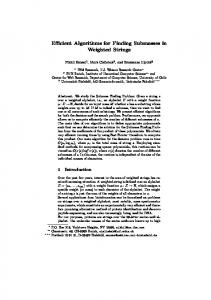
Streaming hidden group with two waves of planning (a). Streaming group without message content – only time, sender id and receiver id are available (b). . . . . . . . . . . . . . . . . . . . . . . . . . . . . . . .

2

1.2

Group structure in Fig. 1.1 . . . . . . . . . . . . . . . . . . . . . . . . . .

3

2.1

Hypothetical group. . . . . . . . . . . . . . . . . . . . . . . . . . . . . . . 11

3.1

Maximum matching algorithm for chains and ordered siblings (a); Maximum matching algorithm for unordered siblings (b). In the algorithms above, we initialize i = 0; j = 1 (i, j are time list positions), and P1 , . . . , Pn = 0 (Pk is an index within Lk ). Let ti = Li [Pi ] and tj = Lj [Pj ]. 17

3.2

Step function on the left and a General Response Functions for 2D Matching on the right . . . . . . . . . . . . . . . . . . . . . . . . . . . . 20

3.3

Algorithm to discover a maximum weighted matching which obeys the causality constraint. In the algorithm above, we initialize i = 0; j = 0 (i, j are time positions in lists L1 = {t1 , t2 , . . . , tn } and L2 = {s1 , s2 , . . . , sm }. 22

3.4

Example of a communication tree structure

3.5

Algorithms used for Querying a Tree T in the data D. In the algorithms above, Drem represents D in an way that allows the Tree-Mine Algorithm to efficiently access the necessary data. . . . . . . . . . . . . 30

3.6

SIGHTS Startup Window. . . . . . . . . . . . . . . . . . . . . . . . . . 34

3.7

SIGHTS System Architecture(currently the link from Chatrooms is not functional) . . . . . . . . . . . . . . . . . . . . . . . . . . . . . . . . . . 35

3.8

Size vs. Density Plot of SIGHTS Sample Analysis (Each dot represents a group, bold dots are groups of high interest level with high amount of communication) . . . . . . . . . . . . . . . . . . . . . . . . . . . . . . . 37

3.9

Graph Clusters Plot of SIGHTS Sample Analysis (Grey dots are actors, each green dot with links to actors represents a group and grey links correspond to background communications) . . . . . . . . . . . . . . . . 38

v

. . . . . . . . . . . . . . . . . 29

3.10

Group Persistence Plot of SIGHTS Sample Analysis (Vertical lines define the time cycles, each rectangle is a group. A selected rectangle is entirely blue, other rectangles are grey if they have no members in common with selected one, partially/entirely green if they have some members in common or partially/entirely blue if a group contains all of the members of the selected rectangle. If the rest of the rectangle is grey it indicates that it has some additional members) . . . . . . . . . . . . . 39

3.11

Clustering on the left has one cluster with 10 members, while the clustering on the right has 2 clusters with 9 and 11 members respectively. . 42

3.12

Steps of the Best Match algorithm while computing symmetric distances between an example of a pair of clusterings . . . . . . . . . . . . . . . . 47

3.13

Results of the K-center algorithm for different values of k . . . . . . . . 48

3.14

Best Match algorithm on the top and K-center algorithm on the bottom. In the algorithms above, let TC1 and TC2 be the number of distinct ′ members of C1 = {S1 , S2 , . . . , Sn } and C2 = {S1′ , S2′ , . . . , Sm } clusterings respectively. Note that both TC1 and TC2 can be computed during the read in or construction of the clusterings. . . . . . . . . . . . . . . . . 49

3.15

Algorithm used to find Communication Probability distance. In the algorithm above, let TC1 be the number of distinct members of C1 = {S1 , S2 , . . . , Sn }. . . . . . . . . . . . . . . . . . . . . . . . . . . . . . . . 52

4.1

Algorithm Conversations used for finding conversations. In the algorithms above, let TCAB be the array of sorted times of messages exchanged between person A and person B. Let C be an intermediate array where we will store times of an ongoing conversation, and let S be a “smoothing” factor, which together with the expected average time difference between messages TABavg determine the suitable distance between consecutive message times in an ongoing conversation C. . . . 59

4.2

Algorithm Propagation Trust used for finding information propagation. In the algorithms above, let D be the set of streaming data and let κsig be the statistical significance threshold found for the dataset D. . . . . 62

5.1

Communications inferred from weblog data. . . . . . . . . . . . . . . . . 66

5.2

The comparison of time intervals, respective thresholds and discovered significant triples. The first column shows the selected [τmin , τmax ], the second column shows the discovered Significance thresholds, and the third column shows the number of significant triples discovered. . . . . . 68

5.3

Relative similarity between the triples discovered on the pair of respective time intervals. . . . . . . . . . . . . . . . . . . . . . . . . . . . . . . 69 vi

5.4

comparison of time intervals, respective thresholds and discovered significant triples. The first column shows the selected [τmin , τmax ], the second column shows the discovered Significance thresholds, and the third column shows the number of significant triples discovered. . . . . . 69

5.5

Step function H and a General Response Function G1 for 2D Matching

5.6

Response Function G2 . . . . . . . . . . . . . . . . . . . . . . . . . . . . 70

5.7

Response Function G3 . . . . . . . . . . . . . . . . . . . . . . . . . . . . 71

5.8

Response Function G4 . . . . . . . . . . . . . . . . . . . . . . . . . . . . 71

5.9

Relative similarity between the groups of H, Gs and G′ s. . . . . . . . . 72

5.10

Distribution of Retweeting delays in Twitter data. The x-axis is the retweet delay in days, y-axis is the number of retweets. . . . . . . . . . 73

5.11

Abundance of triples occurring as a function of frequency of occurrence. (a) chain triples; (b) sibling triples . . . . . . . . . . . . . . . . . . . . 75

5.12

Validation of Weblog group communicational structure on the left against actual friendship links on the right. . . . . . . . . . . . . . . . . . . . . 76

5.13

Comparison of Distances between clusterings of different sizes, discovered in Twitter network over the period of 10 weeks. . . . . . . . . . . . 77

5.14

Evolution of part of the Enron organizational structure from 2000 2002. Note: actors B, C, D, F present in all three intervals. Here is who they are: B - T. Brogan, C - Peggy Heeg, D - Ajaj Jagsi and F Theresa Allen. . . . . . . . . . . . . . . . . . . . . . . . . . . . . . . . 78

5.15

The rate of change of the clusterings in Blogosphere over the period of four weeks. . . . . . . . . . . . . . . . . . . . . . . . . . . . . . . . . . . 79

5.16

The rate of change of the clusterings in the Enron organizational structure from 2000 - 2002. . . . . . . . . . . . . . . . . . . . . . . . . . . . . 79

5.17

The similarity between the trees and the clusterings in the Enron organizational structure from 2000 - 2002. . . . . . . . . . . . . . . . . . . . 80

5.18

The similarity between the trees and the clusterings in the Blogosphere over the period of 4 weeks . . . . . . . . . . . . . . . . . . . . . . . . . 81

5.19

Log plot of the comparison of distance measures used to evaluate a clustering technique used on randomly generated chat data. . . . . . . . 83

5.20

The Significance Threshold results for the time intervals in hours (where τmin = 60 seconds and τmax = number of hours specified in the table) . 84 vii

70

5.21

Comparison of node sets of Conversation and Propagation graphs. The rightmost column and the bottom row contain the sizes of computed graphs, while the numbers at the intersection of the respective row and column represent the number of nodes in common. . . . . . . . . . . . 85

5.22

Comparison of edge sets of Conversation and Propagation graphs. The rightmost column and the bottom row contain the sizes of computed graphs, while the numbers at the intersection of the respective row and column represent the number of edges in common. . . . . . . . . . . . 87

5.23

Statistics on group sizes discovered in the Conversation graphs. Fist column shows the total number of clusters(groups) discovered in the respective graph, while second and third column show the maximum and average cluster(group) size. . . . . . . . . . . . . . . . . . . . . . . 88

5.24

Relative similarity between groups discovered in graphs C and P . . . . 88

5.25

Distance between groups discovered in graph C and randomly generated groups Prand , which in their numbers and sizes mimic P Directed . . . 89

5.26

Number of nodes in common between graphs P , C and the retweeting graph R . . . . . . . . . . . . . . . . . . . . . . . . . . . . . . . . . . . 90

5.27

This table shows the number of nodes in common between graphs by considering the top kP k, kCk and kRk most active users and the node sets of graphs C, P and R . . . . . . . . . . . . . . . . . . . . . . . . . 90

5.28

Percentage of neighbors of the nodes in graphs C and P in common with neighbors in R compared to randomly generated sets and the sets of most active users . . . . . . . . . . . . . . . . . . . . . . . . . . . . . 91

viii

ACKNOWLEDGMENT There are a number of people I would like to thank who have helped me during my doctoral studies. First I would like to thank my advisor Dr. Malik Magdon-Ismail, his guidance, advices and ideas have helped me greatly during all of my Ph.D. years. Also I would like to thank Dr. Mark Goldberg, who provided significant help and insight as well as Dr. William A. Wallace, Professor of Decision Sciences and Engineering Systems, who helped me by providing an important input with respect to the social science side of my research. I enjoyed working with my colleagues Konstantin Mertsalov and Stephen Kelly during these years. Also I would like to thank Dr. Mohammed Zaki for providing his input on tree mining and other data mining aspects of my research. I also enjoyed collaborating with Dr. Boleslaw K. Szymanski and Dr. Sibel Adali on the behavioral trust project. I would also like to thank my family and friends for their support and encouragement. This material is based upon work partially supported by the NSF under Grants DMS-0346341, IIS-0324947, IIS-0634875 and CNS-0323324, by the CIA under A/J 11697, by the ONR under A/J 11707, A 11712, A 11713, by the DIMACSDHS A 40150 through the ONR grant N00014-07-1-0150. Any opinions, findings, and conclusions or recommendations expressed in this material are those of the author(s) and do not necessarily reflect the views of the above mentioned foundations.

ix

ABSTRACT A planning hidden group is a set of individuals planning an activity over a communication medium without announcing their existence. In order to plan, hidden groups need to communicate regularly, possibly in a streaming manner (streaming hidden groups). The hidden group’s communication patterns exhibit structure, which differentiates these communications from random background communications. Here we propose efficient algorithms for identifying streaming hidden group structure by isolating the hidden group’s non-random, planning-related communications from the random background communications. We validate our algorithms on real data (the Enron email corpus and Blog communication data). Analysis of the results reveals that our algorithms extract meaningful hidden group structures. We also present a software system SIGHTS (Statistical Identification of Groups Hidden in Time and Space), which employs the hidden group algorithms and can be used for the discovery, analysis, and knowledge visualization of social coalitions in communication networks such as Blog-networks. The evolution of social groups reflects information flow and social dynamics in social networks. The goal of SIGHTS is to be an assistant to an analyst in identifying relevant information. One of the uses of group detection algorithms is to monitor group dynamics. We develop algorithms to measure similarity between clusterings (sets of sets) which we use to quantify the rate of group evolution. We apply these comparison algorithms to the groups discovered by our algorithms. Trust is an important aspect of groups, and we extend our algorithms to develop two measures of trust which can be used to analyze the “behavioral” trust relationship between people in a social network. We use Twitter network communications for our experimentation and validation of our proposed measures. All the work in this thesis is based on purely statistical analysis of the data, not requiring semantic analysis. This is especially useful in social networks because the volume of information makes semantic analysis intractable. Further, it means that our algorithms are language independent.

x

CHAPTER 1 INTRODUCTION Communication networks (telephone, email, Internet chatroom, etc.) facilitate rapid information exchange among millions of users around the world, providing the ideal environment for groups to plan their activity undetected: their communications are embedded (hidden) within the myriad of unrelated communications. A group may communicate in a structured way while not being forthright about its existence. However, when the group must exchange communications to plan some activity, their need to communicate usually imposes some structure on their communications. We develop statistical and algorithmic approaches for discovering such hidden groups that plan an activity. Hidden group members may have non-planning related communications, be malicious (e.g. a terrorist group) or benign (e.g. a golf foursome). We liberally use “hidden group” for all such groups involved in planning, even though they may not intentionally be hiding their communications. The tragic events of September 11, 2001 underline the need for a tool which aides in the discovery of (malicious) hidden groups during their planning stage, before implementation. One approach to discovering such groups is using correlations among the group member communications. The communication graph of the society is defined by its actors (nodes) and communications (edges). We do not use communication content, even though it can be informative through some natural language processing, because such analysis is time consuming and intractable for large datasets. Our work uses only the time-stamp, sender ID and recipient ID of a message. Our approach to discovering hidden groups is based on the observation that the pattern of communications exhibited by a group pursuing a common objective is different from that of a randomly selected set of actors: any group, even one which tries to hide itself, must communicate regularly to plan. One possible instance of such correlated communication is the occurrence of a repeated communication pattern. Thus, temporal correlation emerges as the members of a group

1

2 00 05 06 12 13 13 15 20 20 22 25 25 31 31

A→C C→F A→B A→B F→G F→H A→C B→D B→E C→F B→D B→E F→G F→H

Golf tomorrow? Tell everyone. Alice mentioned golf tomorrow. Hey, golf tomorrow? Spread the word Tee time: 8am; Place: Pinehurst. Hey guys, golf tomorrow . Hey guys, golf tomorrow . Tee time: 8am; Place: Pinehurst. We’re playing golf tomorrow. We’re playing golf tomorrow. Tee time: 8am; Place: Pinehurst. Tee time: 8am; Place: Pinehurst. Tee time 8am, Pinehurst. Tee time 8am, Pinehurst. Tee off 8am,Pinehurst.

(a)

00 05 06 12 13 13 15 20 20 22 25 25 31 31

A→C C→F A→B A→B F→G F→H A→C B→D B→E C→F B→D B→E F→G F→H

(b)

Figure 1.1: Streaming hidden group with two waves of planning (a). Streaming group without message content – only time, sender id and receiver id are available (b).

need to systematically exchange messages to plan their future activity. This temporal correlation among the group communications will exist throughout the planning stage, which may be some extended period of time. If the planning occurs over a long enough period, this temporal correlation will stand out against a random background of communications and hence can be detected.

1.1

Streaming Hidden Groups In the cyclic hidden group setting [14], all of the hidden group members com-

municate within some characteristic time period, and do so repeatedly over a consecutive sequence of time periods. A streaming hidden group does not obey such strict requirements for its communication pattern. Hidden groups do not necessarily display a fixed time-cycle, during which all members of group members exchange messages, but rather, whenever a step in the planning needs to occur, some hidden group member initiates a communication, which percolates through the hidden group. The hidden group problem may still be formulated as one of finding repeated (possibly overlapping) communication patterns. An example of a streaming hidden group is illustrated in Figure 1.1(a) with a group planning their golf game. Given

3 the message content, it is easy to identify two “waves” of communication. The first wave (in darker font) establishes the golf game; and, the second wave (in lighter font) finalizes the game details. Based on this data, it is not hard to identify the group and conclude that the “organizational structure” of the group is represented in Figure 1.2 to the right (each actor is represented by their first initial). The challenge, once again, is to deduce this same information from the communication stream without the message contents Figure 1.1(b). Two features that distinguish the stream from the cycle model are: (i) communication waves may overlap, as in Figure 1.1(a); (ii) waves may have different durations, some considerably longer than others. The first feature may result in bursty waves of intense communication (many overlapping waves) followed by periods of silence. Such a type of communication dynamics is hard to detect in the cycle model, since all the (overlapping) waves of communication may fall in one cycle. The second can be quantified by a propagation delay function which specifies how much time may elapse between a hidden group member receiving the message and forwarding it to the next member; sometimes the propagation delays may be large, and sometimes small. One would typically expect that such a streaming model would be appropriate for hidden A

groups with some organizational structure as illustrated in the tree in Figure 1.2. We present algorithms which not only discover the streaming hidden group, but also its organizational

B D

structure without the use of message content.

C E

F G

H

We use the notion of communication frequency in order to distinguish nonrandom behavior. Thus, if a group of actors communicates unusually often using the same chain of communication, i.e. the structure of their communications persists

Figure 1.2: Group structure in Fig. 1.1

through time, then we consider this group to be statistically significant and indicative of a hidden group. We present algorithms to detect small frequent tree-like structures, and build larger hidden structures starting from the small ones.

4

1.2

Our Contributions We present efficient algorithms which not only discover the streaming hidden

group, but also its organizational structure without the use of message content. We use the notion of communication frequency in order to distinguish non-random behavior. Thus, if a group of actors communicates unusually often using the same chain of communication, i.e. the structure of their communications persists through time, then we consider this group to be statistically anomalous. We present algorithms to detect small frequent tree-like structures, and build hidden structures starting from the small ones. We propose an approach that uses new cluster matching algorithms together with a sliding window technique to track and observe the evolution of hidden groups over time [10, 31]. We also present a general query algorithm which can determine if a given hidden group (represented as a tree) occurs frequently in the communication stream. All our algorithms have been implemented in a software system SIGHTS (Statistical Identification of Groups Hidden in Time and Space), which employs the hidden group algorithms and can be used for the discovery, analysis, and knowledge visualization of social coalitions in communication networks such as Blog-networks [9]. Additionally, we propose efficient algorithms to obtain the frequency of general trees and to enumerate all statistically significant general trees of a specified size and frequency. We compare these algorithms with the heuristic algorithms above, using the proposed similarity measures [32] to verify that a discovered tree-like structure actually occurs frequently in the data [26]. Our algorithms assume a propagation delay function which characterizes how long it takes for a planning-related message to be propagated along the chain of communication. For a step-propagation delay function, our algorithms are linear time. For more general propagation delay functions, we provide efficient algorithms using flow based matching. We validate our algorithms on the Enron email corpus, as well as the Blog communication data. We present new algorithms to statistically measure “behavioral trust” in the social networks, again using no semantic information. This work is based on a similar

5 premise to finding groups - trust can be measured by how often people communicate and forward. We validate our results on the real data gathered from Twitter network [5]. Thesis Organization. Next, we consider related work, followed by the methodologies for finding streaming hidden groups and tree mining in Chapter 3. Then we present the software system SIGHTS in Chapter 3.5, followed by Chapter 3.6 on similarity measures for clusterings. The algorithms for discovering trust in the social network are presented in Chapter 4. Experiments and validation results can be found in Chapter 5. We conclude in Chapter 6.

1.3

Related Work The approaches of solving the problem of identifying communities and groups

in a social network can be separated into four main areas: • Identifying Groups and Coalitions in Networks by analyzing Message Content Requires Message Content for Analysis Can be Computationally Intensive • Discovering Structure in Networks using Clustering and Partitioning techniques Focuses on Static, Non-Planning Groups May not Allow Multiple Membership for a Node • Models for Social Network Evolution and Infrastructure Mainly Deals with Infrastructure Models Does not Analyze Communication Behavior • Discovering Planning Groups in a Cyclic Model Group’s Communication is Restricted to a Cycle Approaches which analyze message content in order to discover groups in the communication networks are computationally expensive; in addition, such methods require the content of the messages, which can be in different languages, encrypted

6 or unavailable. We now describe in detail the most related work on discovering groups and coalitions. 1.3.1

Discovering Structure using Clustering and Partitioning One of the earliest works [37], on partitioning graphs is by B. W. Kernighan

and S. Lin. They consider the problem of partitioning a weighted graph into subsets of given sizes so as to minimize the sum of the weights on edges cut. Their heuristic method is effective in finding optimal partitions, and fast enough to be practical in solving large problems. In [33], B. Hendrickson and R. Leland extend the work of B. W. Kernighan and S. Lin. They present a multilevel algorithm for graph partitioning in which the graph is approximated by a sequence of increasingly smaller graphs. The smallest graph is then partitioned using a special method, and this partition is propagated back through the hierarchy of graphs. A variant of the Kernighan-Lin algorithm is applied periodically to refine the partition. G. Karypis and V. Kumar propose a multilevel k-way partitioning scheme for irregular graphs. They present a class of graph partitioning algorithms that reduce the size of the graph by collapsing vertices and edges, find a k-way partitioning of the smaller graph, and then refine it to construct a k-way partitioning for the original graph. Their experiments show that their scheme produces partitions that are of comparable or better quality than those produced by the multilevel bisection algorithm, and they also prove their algorithms runtime to be significantly better. In [6], F. R. Bach and M. I. Jordan present a class of algorithms that find clusters using independent component analysis. They assume a linear transformation of the components into clusters, whose elements are dependent on each other and at the same time independent of variables in different clusters. In order to find such clusters, they look for a transformation that fits the estimated sources to a forest-structured graphical model. In [25], G. W. Flake, R. E. Tarjan, and K. Tsioutsiouliklis introduce graph clustering methods based on minimum cuts within the graph. These methods are well suited for graphs where the link structure implies a notion of reference, similarity

7 or endorsement, such as Web and citation graphs. The authors show that the quality of the produced clusters is bounded by strong minimum cut and expansion criteria. They also develop a framework for hierarchical clustering and present applications to real-world data. In [35], R. Kannan, S. Vempala and A. Vetta develop a natural bi-criteria measure for assessing the quality of a clustering that avoids the drawbacks of existing methods. A simple recursive heuristic is shown to have poly-logarithmic worst-case guarantees under the new measure. The main result of the article is the analysis of the spectral algorithm. One variant of spectral clustering turns out to have effective worst-case guarantees, while another finds a “good” clustering, if one exists. In [11, 12], J. Baumes, M. Goldberg and et al. present a methodology for finding communities by clustering a graph into overlapping subgraphs. They define a community as a subset of actors who induce a locally optimal subgraph with respect to a density function defined on a subset of actors. Overlapping communities may be obtained due to the fact that two different subsets with significant overlap may both be locally optimal. The authors design, implement and test two algorithms, RaRe and IS, which find communities according to the corresponding definition. The knowledge of the structure of the communities, as well as the evolution of society as a whole and the evolution of its individual members are considered to be of great importance for discovering groups of actors that hide their communications, perhaps for malicious reasons. Articles [18] and [7] on the other hand examine local community structure in networks, as well as local methods for detecting communities. These methods do not require that we know the entire graph. In [18], A. Clauset defines both a measure of local community structure and an algorithm that infers the hierarchy of communities that enclose a given vertex by exploring the graph one vertex at a time. He shows that on computergenerated graphs, this methodology compares favorably to algorithms that require global knowledge. In [7], J.P. Bagrow and E. M. Bolt present a different method of community detection that is computationally inexpensive. Experiments on several artificial and real-world networks were introduced, including the Zachary karate club.

8 In [53], M. E. J. Newman focuses on large complex networks, such as the Internet, social networks and biological networks. He reviews developments of techniques and models to help understand or predict the behavior of the above mentioned systems, such as the small world effect, degree distributions, clustering, network correlations, random graph models of network growth and preferential attachment, and dynamical processes taking places on the networks. 1.3.2

Models for Social Network Evolution and Infrastructure In this section we will cover more comprehensive models of societal evolu-

tion and simulation, which primarily deal with dynamic models for social network infrastructure, rather than the dynamics of the actual communication behavior. In [60], A. Sanil, D. Banks and K. Carley present explicit probability models for networks that change over time, covering a range of simple but significant qualitative behavior. Maximum likelihood estimates of model parameters which describe the rate of change of the network are derived, and some of their sampling properties are unveiled. In order to calculate these estimates, the researcher must have measurements upon the trajectory of a network, these are the values of a network at successive time points. The authors also describe “goodness of fit” tests for assessing model adequacy, and use Newcombs dataset to illustrate the methodology. In [62] D. Siebecker develops an abstract statistical model of the evolution of social networks. He specifies a set of general models that govern the behavior of these networks on a micro-scale level and observe the resulting emergent macro-scale behavior. The models are general enough to accommodate established theories of social networks, but at the same time flexible enough to accommodate many more possibilities, so as to be applicable to the analysis of email networks, corporate networks, communications networks and social networks. The authors models social groups from the probabilistic actions of a node rather than from the probabilistic network point of view. Since the concept of a set of nodes is utilized, as opposed to a specific structure of nodes, this algorithm can be used to model structure as well as usage. A couple more methodologies on statistical modeling of social groups and quantifying the social group evolution can be found in [27] and [54].

9 G. Palla and et al. uncover the overlapping community structure of complex networks in nature and society. In their article [54] they describe complex systems in terms of networks capturing the intricate web of connections among the units they are made of. After defining a set of new characteristic quantities, they apply an efficient technique for exploring overlapping communities on a large scale. They find that overlaps are significant, and the distributions they introduce reveal universal features of networks. Their studies show that the web of communities has non-trivial correlations and specific scaling properties. In 2006, G. Kossinets and D. Watts conducted an empirical analysis of an evolving social network [38]. They analyze a dynamic social network in which interactions between individuals are inferred from time-stamped email headers, matched with affiliations and attributes. They found that network evolution is dominated by a combination of effects arising from the network topology itself and the organizational structure in which the network is embedded. In the absence of global perturbations, the average network properties appear to approach an equilibrium state, whereas the individual properties are unstable. 1.3.3

Discovering Secret Societies and Cyclic Hidden Groups Erickson, [23], was one of the first to study secret societies. His focus was

also on general communication structure. Since the September 11, 2001 terrorist plot, discovering hidden groups became a topic of intense research. For example it was understood that Mohammed Atta was central to the planning, but that a large percent of the network would need to be removed to render it inoperable [64, 39]. Krebs, [39] identified the network as sparse, which renders it hard to discover through clustering in the traditional sense (finding dense subsets). Our work on temporal correlation would address exactly such a situation. It has also been observed that terrorist group structure may be changing [58], and our methods are based on connectivity alone which is immune to this trend in the finer structure. We assume that message authorship is known, which may not be true (e.g. anonymous web forum postings). Abbasi and Chen propose techniques to address this issue, [2]. The approaches to focus on planning hidden groups were initiated in [45],

10 where Hidden Markov models are the basis for discovering such groups. The underlying methodology is based on random graphs [16, 34] and some of the results on cyclic hidden groups were presented in [14]. In our work we incorporate some of the prevailing social science theories, such as homophily [49], by incorporating group structure. Additionally, there are approaches employing graphlet mining as in [56, 48], where N. Przulj and et al. use the idea of mining graphlets and considering their degree distributions for comparing local structures of node neighborhoods that demonstrates that in protein-protein interaction networks, biological function of a node and its local network structure are closely related. The idea of graphlet mining is very similar to finding groups in a cyclic model, where each graphlet pattern is a group and the data is a sequence of graphs (each graph represents a separate time cycle). Our work is novel because we detect hidden groups by only analyzing communication intensities (and not message content) as well as we remove the idea of time cycles and view the entire data stream as a whole. The study of streaming hidden groups was initiated in [10], which contains some preliminary results. We extend these results in [26, 32] and present a general query algorithm which can determine if a given hidden group (represented as a tree) occurs frequently in the communication stream. We then extended our methodology and developed efficient algorithms to obtain the frequency of general trees and to enumerate all statistically significant general trees of a specified size and frequency. Such algorithms are used in conjunction with the heuristic algorithms to verify that a discovered tree-like structure actually occurs frequently in the data. Also we provide algorithms for general scoring functions for the matching problem and validate our algorithms on a wider range of data.

CHAPTER 2 PROBLEM STATEMENT A hidden group communication structure can be represented by a directed graph. Each vertex is an actor and every edge shows the direction of the communication. For example a hierarchical organization structure could be represented by a directed tree. The graph in Figure 2.1 to the right is an example

A tAC

tAB

B

tBC

tBD

C tCD

D

of a communication structure, in which actor A “simultaneously” sends messages to B and C; then, after receiving the message from A, B sends messages to C and D; C sends a message to D after receiving the messages from A and B. Ev-

Figure 2.1:

Hy-

pothetical group.

ery graph has two basic types of communication structures: chains and siblings. A chain is a path of length at least 3, and a sibling is a tree with a root and two or more children, but no other nodes. Of particular interest are chains and sibling trees with three nodes, which we denote triples. For example, the chains and sibling trees of size three (triples) in the communication structure above are: A → B → D; A → B → C; A → C → D; B → C → D; A → (B, C); and, B → (C, D). We suppose that a hidden group employs a communication structure that can be represented by a directed graph as above. If the hidden group is hierarchical, the communication graph will be a tree. The task is to discover such a group and its structure based solely on the communication data. If a communication structure appears in the data many times, then it is likely to be non-random, and hence represent a hidden group. To discover hidden groups, we will discover the communication structures that appear many times. We thus need to define what it means for a communication structure to “appear”. Specifically, we consider chain and sibling triples (trees of size three). For a chain A → B → C to appear, there must be communication A → B at time tAB and a communication B → C at time tBC such that (tBC − tAB ) ∈ [τmin , τmax ]. This intuitively represents the notion of causality, where A → B “causes” B → C within

11

12 some time interval specified by [τmin , τmax ]. A similar requirement holds for the sibling triple A → B, C; the sibling triple appears if there exists tAB and tAC such that (tAB − tAC ) ∈ [−δ δ]. This constraint represents the notion of A sending messages “simultaneously” to B and C within a small time interval of each other, as specified by δ. For an entire graph (such as the one above) to appear, every chain and sibling triple in the graph must appear using a single set of times. For example, in the graph example above, there must exist a set of times, {tAB , tAC , tBC , tBD , tCD }, which satisfies all the six chain and sibling constraints: (tBD − tAB ) ∈ [τmin , τmax ], (tBC − tAB ) ∈ [τmin , τmax ], (tCD − tAC ) ∈ [τmin , τmax ], (tCD − tBC ) ∈ [τmin , τmax ], (tAB − tAC ) ∈ [−δ, δ] and (tBD − tBC ) ∈ [−δ, δ]. A graph appears multiple times if there are disjoint sets of times each of which is an appearance of the graph. A set of times satisfies a graph if all chain and sibling constraints are satisfied by the set of times. The number of times a graph appears is the maximum number of disjoint sets of times that can be found, where each set satisfies the graph. Causality requires that multiple occurrences of a graph should monotonically increase in time. Specifically, if tAB “causes” tBC and t′AB “causes” t′BC with t′AB > tAB , then it should be that t′BC > tBC . In general, if we have two disjoint occurrences (sets of times) {t1 , t2 , . . .} and {s1 , s2 , . . .} with s1 > t1 , then it should be that si > ti for all i. A communication structure which is frequent enough becomes statistically significant when its frequency exceeds the expected frequency of such a structure from the random background communications. The goal is to find all statistically significant communication structures, which is formally stated in the following algorithmic problem statement. Input: A communication data stream and parameters: δ, τmin , τmax , h, κ. Output: All communication structures of size ≥ h, which appear at least κ times, where the appearance is defined with respect to δ, τmin , τmax . Assuming we can solve this algorithmic task, the statistical task is to determine h and κ to ensure that all the output communication structures reliably correspond to non-random “hidden groups”. We first consider small trees, specifically chain and sibling triples. We then develop a heuristic to build up larger hidden groups from clusters of triples. Additionally we mine all of the frequent directed acyclic graphs

13 and propose new ways of measuring the similarity between sets of overlapping sets. We obtain evolving hidden groups by using a sliding window in conjunction with the proposed similarity measures to determine the rate of evolution.

CHAPTER 3 ALGORITHMS FOR DISCOVERING STREAMING HIDDEN GROUPS AND THEIR STRUCTURE 3.1

Algorithms for Chain and Sibling Trees We will start by introducing a technique to find chain and sibling triples,

i.e. trees of type A → B → C (chain) and trees of type A → (B, C) (sibling). To accomplish this, we will enumerate all the triples and count the number of times each triple occurs. Enumeration can be done by brute force, i.e. considering each possible triple in the stream of communications. We have developed a general algorithm for counting the number of occurrences of chains of length ℓ, and siblings of width k. These algorithms proceed by posing the problem as a multi-dimensional matching problem, which in the case of tipples becomes a two-dimensional matching problem. Generally multi-dimensional matching is hard to solve, but in our case the causality constraint imposes an ordering on the matching which allows us to construct a linear time algorithm. Finally we will introduce a heuristic to build larger graphs from statistically significant triples using overlapping clustering techniques [11]. 3.1.1

Computing the Frequency of a Triple Consider the triple A → B → C and the associated time lists L1 = {t1 ≤ t2 ≤

. . . ≤ tn } and L2 = {s1 ≤ s2 ≤ · · · ≤ sm }, where ti are the times when A sent to B and si the times when B sent to C. An occurrence of the triple A → B → C is a pair of times (ti ,si ) such that (si − ti ) ∈ [τmin τmax ]. Thus, we would like to find the maximum number of such pairs which satisfy the causality constraint. It turns out that the causality constraint does not affect the size of the maximum matching, however it is an intuitive constraint in our context. We now define a slightly more general maximum matching problem: for a pair (ti , si ) let f (ti , si ) denote the score of the pair. Let M be a matching {(ti1 , si1 ), (ti2 , si2 ) . . . (tik , sik )} of size k. We define the score of M to be 14

15

Score(M ) =

k X

f (tij , sij ).

j=1

The maximum matching problem is to find a matching with a maximum score. The function f (t, s) captures how likely a message from B → C at time s was “caused” by a message from A → B at time t. In our case we are using a hard threshold function   1 if t − s ∈ [τ , τ ], min max f (t, s) = f (t − s) =  0 otherwise.

The matching problem for sibling triples is identical with the choice   1 if t − s ∈ [−δ, δ], f (t, s) = f (t − s) =  0 otherwise.

We can generalize to chains of arbitrary length and siblings of arbitrary width as follows. Consider time lists L1 , L2 , . . . ,Lℓ−1 corresponding to the chain A1 → A2 → A3 → · · · → Aℓ , where Li contains the sorted times of communications Ai → Ai+1 . An occurrence of this chain is now an ℓ − 1 dimensional matching {t1 , t2 , . . . , tℓ−1 } satisfying the constraint (ti+1 − ti ) ∈ [τmin τmax ] ∀ i = 1,· · · ,ℓ − 2. The sibling of width k breaks down into two cases - ordered siblings which obey constraints similar to the chain constraints, and unordered siblings. Consider the sibling tree A0 → A1 , A2 , · · · Ak with corresponding time lists L1 , L2 , . . . ,Lk , where Li contains the times of communications A0 → Ai . Once again, an occurrence is a matching {t1 , t2 , . . . , tk }. In the ordered case the constraints are (ti+1 − ti ) ∈ [−δ δ]. This represents A0 sending communications “simultaneously” to its recipients in the order A1 , . . . , Ak . The unordered sibling tree obeys the stricter constraint (ti − tj ) ∈ [−(k − 1)δ, (k − 1)δ], ∀ i, j pairs, i 6= j. This stricter constraint represents A0 sending communications to its recipients “simultaneously” without any particular order. Both problems can be solved with a greedy algorithm. The detailed algorithms for arbitrary chains and siblings are given in Figure 3.1(a). Here we sketch the al-

16 gorithm for triples. Given two time lists L1 ={t1 , t2 , . . . , tn } and L2 ={s1 , s2 , . . . , sm } the idea is to find the first valid match (ti1 , si1 ), which is the first pair of times that obey the constraint (si1 − ti1 ) ∈ [τmin τmax ], then recursively find the maximum matching on the remaining sub lists L′1 = {ti1 +1 , . . . , tn } and L′2 = {si1 +1 , . . . , sm }. The case of general chains and ordered sibling trees is similar. The first valid match is defined similarly. Every pair of entries tLi ∈ Li and tLi+1 ∈ Li+1 in the maximum matching must obey the constraint (tLi+1 − tLi ) ∈ [τmin τmax ]. To find the first valid match, we begin with the match consisting of the first time in all lists. Denote these times tL1 , tL2 , . . . , tLℓ . If this match is valid (all consecutive pairs satisfy the constraint) then we are done. Otherwise consider the first consecutive pair to violate this constraint. Suppose it is (tLi , tLi+1 ); so either (tLi+1 − tLi ) > τmax or (tLi+1 − tLi ) < τmin . If (tLi+1 − tLi ) > τmax (tLi is too small), we advance tLi to the next entry in the time list Li ; otherwise (tLi+1 − tLi ) < τmin (tLi+1 is too small) and we advance tLi+1 to the next entry in the time list Li+1 . This entire process is repeated until a valid first match is found. An efficient implementation of this algorithm is given in Figure 3.1. The algorithm for unordered siblings follows a similar logic. The next theorem gives the correctness of the algorithms. Theorem 1 Algorithm-Chain and Algorithm-Sibling find maximum matchings. Proof: By induction. Given a set of time lists L = (L1 , L2 , . . . , Ln ) our algorithm produces a matching M = (m1 , m2 , . . . , mk ), where each matching mi is a sequence of n times from each of the n time lists mi = (ti1 , ti2 , . . . , tin ). Let M ∗ = (m∗1 , m∗2 , . . . , m∗k∗ ) be a maximum matching of size k ∗ . We prove that k = k ∗ by induction on k ∗ . The next lemma follows directly from the construction of the Algorithms. Lemma 1 If there is a valid matching our algorithm will find one. Lemma 2 Algorithm-Chain and Algorithm-Sibling find an earliest valid matching. Let the first valid matching found by either algorithm be m1 = (t1 , t2 , . . . , tn ), then for any other valid matching m′ = (s1 , s2 , . . . , sn ) ti ≤ si ∀ i = 1, · · · , n.

17 1: Algorithm Chain 2: while Pk ≤ kLk k − 1, ∀k do 3: if (tj − ti ) < τmin then 4: Pj ← Pj + 1 5: else if (tj − ti ) ∈ [τmin , τmax ] 6: 7: 8: 9: 10: 11: 12: 13: 14:

then if j = n then (P1 , . . . , Pn ) is the match Pk ← Pk + 1, ∀k i ← 0; j ← 1 else i ← j; j ← j + 1 else Pi ← Pi + 1 j ← i; i ← i − 1 (a)

next

1: Algorithm Sibling 2: while Pk ≤ kLk k − 1, ∀k do 3: if (tj − ti ) < −(k − 1)δ then 4: Pj ← Pj + 1 5: else if (tj − ti ) > (k − 1)δ, ∀i < j 6: 7: 8: 9: 10: 11: 12: 13: 14:

then Pi ← Pi + 1 j ←i+1 else if j = n then (P1 , . . . , Pn ) is match Pk ← Pk + 1, ∀k i ← 0; j ← 1 else j ←j+1

the

next

(b)

Figure 3.1: Maximum matching algorithm for chains and ordered siblings (a); Maximum matching algorithm for unordered siblings (b). In the algorithms above, we initialize i = 0; j = 1 (i, j are time list positions), and P1 , . . . , Pn = 0 (Pk is an index within Lk ). Let ti = Li [Pi ] and tj = Lj [Pj ].

Proof: Proof by contradiction. Assume that in m1 and m′ there exists a corresponding pair of times s < t and let si , ti be the first such pair. Since m1 and m′ are valid matchings, then si and ti obey the constraints: τmin ≤ (ti+1 − ti ) ≤ τmax , τmin ≤ (ti − ti−1 ) ≤ τmax and τmin ≤ (si+1 − si ) ≤ τmax , τmin ≤ (si − si−1 ) ≤ τmax . Since si < ti , then τmin < (ti+1 − si ) and τmax > (si − ti−1 ). Also because si−1 ≥ ti−1 , we get that τmin ≤ (si − ti−1 ) and since (si+1 − si ) ≤ τmax , then (min(ti+1 , si+1 ) − si ) ≤ τmax as well. But if si satisfies the above conditions, then m1 would not be the first valid matching, because the first matching mf would contain mf = (t1 , t2 , . . . , ti−1 , si , min(ti+1 , si+1 ), min(ti+2 , si+2 ), . . . , min(tn , sn )). Let us show this by induction on the number of pairs p of the type min(ti+j , si+j ), where si < ti and j ≥ 1. If p = 1, then j = 1, and since τmin ≤ (si+1 − si ) ≤ τmax and τmin < (ti+1 − si ), then τmin < (min(ti+1 , si+1 )−si ) ≤ τmax as well, and therefore satisfies the matching constraints.

18 Let the matching constraints be satisfied up to p = m, such that in the matching m∗ = (t1 , t2 , . . . , ti−1 , si , min(ti+1 , si+1 ), . . . , min(ti+m , si+m ), . . . , min(tn , sn )) the sequence of elements of m∗ up to min(ti+m , si+m ) satisfy the matching constraints. Then we can show that min(ti+m+1 , si+m+1 ) is also a part of the matching. Since m1 and m′ are both valid matchings, then τmin ≤ (ti+m+1 − ti+m ) ≤ τmax and τmin ≤ (si+m+1 − si+m ) ≤ τmax , from which we get that τmin ≤ (min(ti+m+1 , si+m+1 ) − min(ti+m , si+m )) ≤ τmax . Thus, min(ti+m+1 , si+m+1 ) is also a part of the matching. Consequently, we get a contradiction since mf would be an earlier matching if there exists a pair of times si < ti . Therefore, Algorithm-Chain and AlgorithmSibling find an earliest valid matching. If k ∗ = 0, then k = 0 as well. If k ∗ = 1, then there exists a valid matching and by Lemma 1 our algorithm will find it. Suppose that for all sets of time lists for which k ∗ = M , the algorithm finds matchings of size k ∗ . Now consider a set of time lists L = (L1 , L2 , . . . , Ln ) for which an optimal algorithm produces a maximum matching of size k ∗ = M + 1 and consider the first matching in this list (remember that by the causality constraint, the matchings can be ordered). Our algorithm constructs the earliest matching and then recursively processes the remaining lists. By Lemma 2, our first matching is not later than optimal’s first matching, so the partial lists remaining after our first matching contain the partial lists after optimal’s first matching. This means that the optimal matching for our partial lists must be M . By the induction hypothesis our algorithm finds a matching of size M on these partial lists for a total matching of size M + 1. For a given set of time lists L = (L1 , L2 , . . . , Ln ) as input, where each Li has P a respective size di , define the total size of the data as kDk = ni=1 di .

Theorem 2 Algorithm-Chain runs in O(kDk) time.

Proof: When looking for a matching, we compare a pair of elements from two time lists. For each comparison, we increment at least once in a time list if the comparison failed. After n − 1 successful comparisons, we increment in every time

19 list by one. Thus there can be at most O(kDk) failed comparisons and O(kDk) successful comparisons, since there are kDk list advances in total. Theorem 3 Algorithm-Sibling runs in O(n · kDk) time. Proof: As in Algorithm-Chain a failed comparison leads to at least one increment,
but now n2 successful comparisons are needed before incrementing in every time list. Therefore, in the worst case O(n2 ) comparisons lead to O(n) list advances.

Since there are at most kDk list advances, the maximum number of comparisons is O(n · kDk) 3.1.2

Finding all Triples Assume the data are stored in a vector. Each component in the vector corre-

sponds to a sender id and stores a balanced search tree of receiver lists (indexed by a receiver id). And let S be the whole set of distinct senders. The algorithm for finding chain triples considers sender id s and its list of receivers {r1 , r2 , · · · , rd }. Then for each such receiver ri that is also a sender, let {ρ1 , ρ2 , · · · , ρf } be the receivers to which ri sent messages. All chains beginning with s are of the form s → ri → ρj . This way we can more efficiently enumerate the triples (since we ignore triples which do not occur). For each sender s we count the frequency of each triple s → ri → ρj . Theorem 4 Algorithm to find all triple frequencies takes O(kDk + n · kDk) time. Proof: To find all of the chain triples requires O(kDk) computations, and to find all of the sibling triples similarly requires O(n · kDk) computations. Therefore, the total number of operations needed is O(kDk + n · kDk). 3.1.3

General Scoring Functions for 2D-Matching One can observe that for our 2D-matching we are using a so called “Step

Function”, which returns 1 for values between [τmin , τmax ], and gives 0 otherwise. Such a function represents the probability delay density which is the distribution of the time it takes to propagate a message once it is received. Here we extend our matching algorithm to be able to use any general propagation delay density function, see Figure 3.2.

20

Figure 3.2: Step function on the left and a General Response Functions for 2D Matching on the right Usage of these various functions may uncover some additional information about the streaming groups and their structure which the “Step Function” missed. Unfortunately, the matching problem with an arbitrary function, unlike in the case with the “Step Function” which can be solved in linear time, cannot be solved so efficiently. First we provide an efficient algorithm to find a 2D maximum matching which satisfies a causality constraint (a maximum weight matching which has no intersecting edges). Additionally we will provide an approach involving the Hungarian algorithm to discover a maximum weighted 2D-matching, which does not obey the causality constraint (edges involved in the maximum matching may intersect). Given the two time lists L1 = {t1 , t2 , . . . , tn } and L2 = {s1 , s2 , . . . , sm } and a general scoring function f (·) over the specified time interval [τmin,τmax ] we would like to find a maximum weighted 2d matching between these two time lists, such that the matching has no intersecting edges. No intersecting edges intuitively guaranties the causality constraint. To solve this problem we will employ the dynamic programming approach. Let Mi,j be a maximum matching with the respective weight w(Mi,j ), obeying the causality constraint, involving up to and including the ti ’th item of the list L1 and up to and including the sj ’th item in the list L2 . Thus, the matching Mn,m will hold the maximum weighted matching for the entire lists L1 and L2 . When we compute the matching, we attempt to improve it from step to step by adding only the edges(matches) which do not intersect any of the edges already present in the matching. The following description of the algorithm will show why it is the

21 case. We will illustrate now that if we have correct solutions to subproblems Mi−1,j , Mi,j−1 and Mi−1,j−1 , then we can construct a maximum matching Mi,j , which obeys the causality constraint by considering the following two simple cases: 1. Either the elements ti and sj are both matched to each other in the matching Mi,j , in which case Mi,j = Mi−1,j−1 ∪ (ti , sj ). Obviously the edge (ti , sj ) does not intersect any of the previous edges of Mi−1,j−1 so we maintain the causality constraint; 2. Or, the elements ti and sj are not matched to each other in the matching Mi,j . Then, one of the ti or sj is not matched (see Lemma 4), which means that Mi,j = max{Mi,j−1 , Mi−1,j }. No edges are added to the matching in this case. We initialize our algorithm by computing in linear time the base set of matches {M1,1 , M1,2 , . . . , M1,n } (the bottom row) and {M1,1 , M2,1 , . . . , Mm,1 } (the left most column) of the two-dimensional array of subproblems (of size n · m) that is being built up. The matchings {M1,1 , M1,2 , . . . , M1,n } are constructed by taking the first element s1 from the list L2 and computing all of the weights of the edges w(ti , s1 ), s.t. w(M1,1 ) = {f (s1 − t1 )} (contains edge (t1 , s1 ), if its not 0), w(M1,2 ) = max{f (s1 − t1 ), f (s1 − t2 )} (contains the heavier of two edges (t1 , s1 ), (t2 , s1 ) ) up to M1,n = max{f (s1 − t1 ), f (s1 − t2 ), . . . , f (s1 − tn )} (contains the edge of maximum weight considered over all ti ’s). We similarly compute the set of matchings {M1,1 , M2,1 , . . . , Mm,1 }. Next we are ready to fill in the rest of the two-dimensional array of subproblems starting with M2,2 , since M1,1 , M1,2 and M2,1 are all available. The pseudo code of the algorithm is given in Figure 3.3. Lemma 3 The matching constructed by algorithm Match-Causality, obeys the causality constraint (contains no intersecting edges). Proof: By construction of our algorithm, during the computation of every Mi,j a new edge is added to the matching only if the (Mi−1,j−1 ∪ (ti , sj )) is picked as maximum. But since ti and sj are the very last two elements for the matching Mi,j , they can’t intersect any of the edges. Thus, since at each step our algorithm

22

1: 2: 3: 4: 5: 6: 7:

Algorithm Match-Causality Compute {M1,1 , M1,2 , . . . , M1,n } and {M1,1 , M2,1 , . . . , Mm,1 } for i = 2; i ≤ n; i + + do for j = 2; j ≤ m; j + + do Mi,j = max{w(Mi−1,j−1 ∪ (ti , sj )), w(Mi−1,j ), w(Mi,j−1 )} Store a direction for backtracking Start at Mm,n and backtrack to retrieve the edges of the matching

Figure 3.3: Algorithm to discover a maximum weighted matching which obeys the causality constraint. In the algorithm above, we initialize i = 0; j = 0 (i, j are time positions in lists L1 = {t1 , t2 , . . . , tn } and L2 = {s1 , s2 , . . . , sm }. consistently adds edges which do not intersect any of the previously added edges, the final matching will contain no intersecting edges. Lemma 4 If the items ti and sj are not matched to each other in the matching Mi,j , then one of the ti , sj is not matched at all. Proof: Let us assume for the sake of contradiction that both ti and sj are matched with some nodes. This automatically implies that ti must be matched with some sj ′ , which appears before the sj in the list L2 ; and sj is matched with some ti′ , which occurs before the ti in the list L1 . But this means that the edges (ti , sj ′ ) and (ti′ , sj ) intersect, a contradiction. Theorem 5 Algorithm Match-Causality correctly finds a maximum weighted matching. Proof: Proof by induction. For the base case lets consider the case where kL1 k = 1 and kL2 k = 1, in this case the algorithm will trivially match t1 (the only element of L1 ) with s1 (the only element of L2 ) as long as the f (s1 − t1 ) > 0, otherwise the matching would be empty. For the inductive step we assume that if our algorithm finds all of the maximum weighted matchings ,which obey the causality constraint, correctly up to and including Mi,j−1 , then the algorithm correctly finds the maximum matching which obeys the causality constraint for Mi,j (the very next position it considers after

23 Mi,j−1 ). By our assumption we know that our algorithm correctly found the matchings Mi,j−1 , Mi−1,j−1 and Mi−1,j , which all obey the causality constraint, since all of them occurred before the computation of Mi,j . If so, then our algorithm by construction will pick the maximum weight matching from the set of 3 possible matchings {(Mi−1,j−1 ∪ (ti , sj )), Mi−1,j , Mi,j−1 }, which guaranties the Mi,j to be maximum weight and obey the causality constraint. Theorem 6 Algorithm Match-Causality runs in O(n · m) time. Proof: Computation of the first column and the first row takes O(n + m) time, by simply keeping the track of the running maximum during the computation. Next we compute O(n · m) elements, where each one takes linear time to compute (find the maximum of 3 elements). Thus, the total runtime is O(n · m). The general propagation delay function f (·) can have any shape, and one can wonder if it is possible to find an algorithm which will perform faster then O(n · m) for some special case of the general propagation delay function. Let us consider one of the most intuitive scenarios where the propagation delay function is monotonically decreasing. We prove that there does not exist an algorithm which can construct the maximum weight matching in less then O(n · m) time, which obeys the causality constraint. Theorem 7 Algorithm which finds exactly the maximum weight matching for a propagation delay function which is strictly monotonically decreasing (not a “step” function) and obeys the causality constraint, requires at least O(n · m) time. Proof: Consider the two time lists L1 = {t1 , t2 , . . . , tn }, L2 = {s1 , s2 , . . . , sm }, where every time sj > tn , and a strictly monotonically decreasing function f (·), s.t. f (sm − t1 ) > 0. The first observation to make is that tn must be a part of the matching. If tn′ is the last matched item and tn is not matched, where n′ < n, then the matching can be improved by replacing tn′ with tn , since f (·) is a strictly monotonically decreasing function and n′ < n. Since the matching obeys the causality constraint, then the maximum weight matching can be {f (s1 −tn )} or {f (s2 −tn )+f (s1 −tn−1 )} or . . . or {f (s1 −t1 )+f (s2 −

24 t2 ) + . . . + f (sm − tn )}, order of O(n · m) combinations. And since the function is any strictly monotonically decreasing function, one can not guaranty the optimality of the discovered matching without having to consider all of the mentioned O(n · m) permutations. Thus an algorithm which finds exactly the maximum weight matching for a propagation delay function which is strictly monotonically decreasing (not a “step” function) and obeys the causality constraint, requires at least O(n · m) time.

Additionally we present a method to discover a maximum weight matching for a general propagation delay function, which doesn’t have to obey the causality constraint (we allow the intersection of edges in the matching). The general idea is to use a Hungarian algorithm to find a maximum weighted 2d-matching for a pair of time lists. First, given two time lists L1 = {t1 , t2 , . . . , tn } and L2 = {s1 , s2 , . . . , sm } and a general scoring function f (·) over the specified time interval [τmin,τmax ], we construct the bipartite graph, where on the left we have the set of n nodes, where each node represents a respective time from {t1 , t2 , . . . , tn } and on the right we have a set of m nodes representing each of {s1 , s2 , . . . , sm } times respectively. Each pair of nodes ti and sj is connected by an edge, where the weight on the edge equals to f (sj − ti ) (0 if outside the [τmin,τmax ] bounds). Once we have constructed the bipartite graph we are ready to run the Hungarian algorithm. The produced matching M is of maximum weight, but does not take into account the causality constraint (some of the edges of M may intersect). Theorem 8 Maximum matching which doesn’t have to obey the causality constraint using a general propagation delay function can be computed in O((n + m)3 ) time. Proof: Hungarian algorithm has been shown to run in O(kV k3 ) time, which in our case translates to O((n + m)3 ) operations. We use ENRON data to test general propagation delay functions against the “step” function. The results of our experiments are presented in Section 5.5. It turns out that in most of the cases there is not much added value from the more

25 general propagation delay function in practice. Thus, the more efficient function seems adequate.

3.2

Statistically Significant Triples We determine the minimum frequency κ that makes a triple statistically sig-

nificant, using a statistical model that mimics certain features of the data: we model the inter-arrival time distribution and receiver id probability conditioned on sender id, to generate synthetic data and find all randomly occurring triples to determine the threshold frequency κ. Above this threshold frequency κ, it is unlikely that triples with that frequency appear in the random model. 3.2.1

A Model for the Data We estimate directly from the data the message inter-arrival time distribution

f (τ ) and, for each sender the receiver conditional probability distribution P (r|s), and the marginal distribution P (s) using simple histograms (one histogram for f (τ ), S histograms for P (r|s) and one for P (s)). One may also model additional features (e.g. P (s|r)), to obtain more accurate models. One should however bear in mind that the more accurate the model, the closer the random data is to the actual data, hence the less useful the statistical analysis will be - it will simply reproduce the data. 3.2.2

Synthetic Data Suppose one wishes to generate N messages using f (τ ), P (r|s) and P (s). First

we generate N inter-arrival times independently, which specifies the times of the communications. We now must assign sender-receiver pairs to each communication. The senders are selected independently from P (s). We then generate each receiver independently, but conditioned on the sender of that communication, according to P (r|s).

26 3.2.3

Determining the Significance Threshold To determine the significance threshold κ, we generate M (as large as possible)

synthetic data sets and determine the triples together with their frequencies of occurrence in each synthetic data set. The threshold κ may be selected as the average plus two standard deviations, or (more conservatively) as the maximum frequency of occurrence of a triple.

3.3

Constructing Larger Graphs using Heuristics Now we discuss a heuristic method for building larger communication struc-

tures, using only statistically significant triples. We will start by introducing the notion of an overlap factor. We will then discuss how the overlap factor is used to build a larger communication graph by finding clusters, and construct the larger communication structures from these clusters. 3.3.1

Overlap between Triples For two statistically significant triples (A, B, C) and (D, E, F ) (chain or sib-

ling) with maximum matchings at the times M1 = {(t1 , s1 ), . . . , (tk , sk )} and M2 = {(t′1 , s′1 ), . . . , (t′p , s′p )}, we use an overlap weighting function W (M1 , M2 ) to capture the degree of coincidence between the matchings M1 and M2 . The simplest such overlap weighting function is the extent to which the two time intervals of communication overlap. Specifically, W (M1 , M2 ) is the percent overlap between the two intervals [t1 , sk ] and [t′1 , s′p ]: W (M1 , M2 ) = max



 min(sk , s′p ) − max(t1 , t′1 ) ,0 max(sk , s′p ) − min(t1 , t′1 )

A large overlap factor suggests that both triples are part of the same hidden group. More sophisticated overlap factors could take into account intermittent communication but for our present purpose, we will use this simplest version.

27 3.3.2

The Weighted Overlap Graph and Clustering We construct a weighted graph by taking all significant triples to be the vertices

in the graph. Let Mi be the maximum matching corresponding to vertex (triple) vi . Then, we define the weight of the edge eij to be ω(eij ) = W (Mi , Mj ). Thus, we have an undirected complete graph (some weights may be 0). By thresholding the weights, one could obtain a sparse graph. Dense subgraphs in this graph correspond to triples that were all active at about the same time, and are a candidate hidden group. Thus, we want to cluster the graph into dense possibly overlapping subgraphs. Given the triples in a cluster we can build a directed graph, consistent with all the triples, to represent its communication structure. If a cluster contains multiple connected components, this may imply the existence of some hidden structure connecting them. Below is an outline of the entire algorithm: 1: Obtain the significant triples. 2: Construct a weighted overlap graph (weights are overlap factors between pairs

of triples). 3: Perform clustering on the weighted graph. 4: Use each cluster to determine a candidate hidden group structure.

For the clustering, since clusters may overlap, we use the algorithms presented in [11], [12].

3.4

Algorithm for Querying Tree Hidden Groups We describe efficient algorithms for computing (exactly) the frequency of a

hidden group whose communication structure is an arbitrary pre-specified tree. We assume that messages initiate from the root. The parameters τmin , τmax , δ are also specified. Such an algorithm can be used in conjunction with the previous heuristic algorithms to verify that a discovered tree-like structure actually occurs frequently in the data. Let L be an adjacency list for the tree T , D a dataset in which we will query this tree. The first entry in the list L is the root communicator followed by the list of all its children (receivers) the root sends to. The next entries in L contain the

28 lists of children for each of the receivers of Lroot until we reach the leaves, which have no children. After we have read in D, we process L and use it to construct the tree, in which every node will contain: node id, time list when its parent sent messages to it, and a list of children. We construct such tree by processing L and checking each communicator that has children if it is present in D as a Sender, and if its children are present in D in the list of its Receivers. During the construction, if a node that has children is not present in D as a Sender, or some child is not on the list of Receivers of its parent, then we know that the given tree does not exist in the current data set D and we can stop our search. For a tree to exist there should be at least one matching involving all of the nodes (lists) in the tree. We start with root and consider the time lists of its children. We use Algorithm-Sibling to find the first matching m1 = (t1 , t2 , . . . , tn ), where ti is an element of the i’s child time list and n is the number of time lists. After the first matching m1 is found, we proceed by considering the children in the matching m1 from the rightmost child to the left by taking the value ti , which represents this node in the matching and passing it down to the child node. Next we try to find a matching m2 = (s1 , s2 , . . . , sk ) for the k child time lists using Algorithm-Sibling. There are three cases to consider: 1. Every element sj of the matching m2 also satisfies the chain-constraint with the element ti : τmin ≤ sj − ti ≤ τmax , ∀sj ∈ m2 , j = k, . . . , 1. In this case we say m2 ∼ ti (m2 matches ti ) and proceed by considering all children. Otherwise consider the rightmost sj ∈ m2 . The two cases below refer to sj . 2. If sj < ti + τmin , in which case we say m2 < ti , we advance to the next element in child j’s time list and continue as with Algorithm-Sibling to find the next matching (s′1 , s′2 , . . . , s′k ). This process is repeated as long as m2 < ti . Eventually we will find an m2 with m2 ∼ ti or we will reach the end of some list (in which case there is no further matching) or we come to a matching m2 > ti (see case below). 3. If sj > ti + τmax , in which case we say m2 > ti , we advance ti to the next

29 element in i’s time list on the previous level and proceed as with AlgorithmSibling to find the next matching in the previous level. After this new matching (t′1 , t′2 , . . . , t′n ) is found, the chain constraints have to be checked for these time lists (t′1 , t′2 , . . . , t′n ) with their previous level and the algorithm proceeds recursively from then on.

A L1

3 L7

E

B L8

1 L3

L2

D

C L4

F

G

L5

H

2 L6

I

Figure 3.4: Example of a communication tree structure The entire algorithm for finding a complete matching can be formulated into two steps: find the first matching; recursively process the remaining parts of the time lists. What we have described is the first step which is accomplished by calling the recursive algorithm F indN extrec (N U LL, root) that is summarized in the Figure 3.5. If this returns T RU E, the algorithm has found the first occurrence of the tree, which can be read off from the current time list pointers. After this instance is found, we store it and proceed by considering the remaining part of the time lists starting from the root. To illustrate how the Algorithm Tree-mine works, consider the example tree T in Figure 3.4. Let node A to be a root and let L1 , . . . , L8 be the time lists. Refer to (L1 , L2 , L3 ) as the phase1 lists, (L4 , L5 , L6 ) as the phase2 lists and (L7 , L8 ) as the phase3 lists. Let m1 = (t1 , t2 , t3 ), m2 = (s1 , s2 , s3 ) and m3 = (r1 , r2 ) be the first matchings of the phase1 , phase2 and phase3 lists respectively. If m2 ∼ t3 and m3 ∼ t1 , we have found the first matching and we now recursively process the remaining time lists. Suppose m2 < t3 (eg. s2 < t3 +τmin ), then we move to the next matching in the phase2 lists. If m2 > t3 then we move to the next matching in phase1 lists and reconsider the phase2 matching and the phase3 matching if necessary. If m2 ∼ t3 we then similarly check m3 with t1 . Since node C is a leaf, it need not be

30

1: Algorithm Tree-Mine(T ,D) 2: Drem ← D 3: while M = T RU E do 4: (M, t′ ) = F indN ext(T, Drem ) 5: if M then 6: Store Match 7: Increment List Pointers; get Drem

1: Algorithm F indN ext(T, Drem ) 2: Initialize all truthj ← 0 3: return F indnextrec (N U LL, root)

1: 2: 3: 4: 5: 6: 7: 8: 9: 10: 11: 12: 13: 14:

Algorithm F indN extrec (t, ∗node i) (⋆)Run Algorithm-Sibling from current time list pointers to get m = (t1 , . . . , tn ) if m ∼ t then for j = n to 1 do if (truthj = 1 & prevj < tj ) or truthj = 0 then (truthj , prevj ) = F indN extrec (tj , ∗node j) if truthj = 0 then Increase tj pointer, GOTO(⋆) else return (truthj ,t) if m < t then Increase tj pointer, GOTO(⋆) if m > t then return (0, t)

Figure 3.5: Algorithms used for Querying a Tree T in the data D. In the algorithms above, Drem represents D in an way that allows the Tree-Mine Algorithm to efficiently access the necessary data.

31 further processed. Theorem 9 Algorithm Tree-Mine correctly finds the maximum number of occurrences for a specified tree T . Proof: Proof by contradiction. Given a set of time lists L = (L1 , L2 , . . . , Ln ) that specify a tree, our algorithm produces a matching M = (m1 , m2 , . . . , mk ), where each matching mi is a sequence of n times from each of the n time lists mi = (ti1 , ti2 , . . . , tin ). Let M ∗ = (m∗1 , m∗2 , . . . , m∗k∗ ) be a maximum matching of size k ∗ . The next lemma follows directly from the construction of the Algorithms. Lemma 5 If there is a valid matching our algorithm will find one. Lemma 6 Algorithm Tree-Mine finds an earliest valid matching(occurrence). Let the first valid matching found by our algorithm be m1 = (t1 , t2 , . . . , tn ), then for any other valid matching m′ = (s1 , s2 , . . . , sn ) ti ≤ si ∀ i = 1, · · · , n. Proof: Proof by contradiction. Assume that in m1 and m′ there exists a corresponding pair of times s < t and let si , ti be the first such pair. Since m1 and m′ are valid matchings, then si and ti obey the chain constraints: τmin ≤ (ti − tp ) ≤ τmax (where tp is a time passed down by the parent node), τmin ≤ ((tchildren − ti ) ≤ τmax (where tchildren are times of children of ti ), similarly τmin ≤ (si − sp ) ≤ τmax , τmin ≤ (schildren − si ) ≤ τmax ; and obey the sibling constraint: τmin ≤ (ti+1 − ti ) ≤ τmax , τmin ≤ (ti − ti−1 ) ≤ τmax (where ti−1 and ti+1 are matched times of neighboring siblings of ti ) and similarly τmin ≤ (si+1 − si ) ≤ τmax , τmin ≤ (si − si−1 ) ≤ τmax . Since si < ti , then τmin < (ti+1 − si ) and τmax > (si − ti−1 ). Also because si−1 ≥ ti−1 , we get that τmin ≤ (si − ti−1 ) and since (si+1 − si ) ≤ τmax , then (min(ti+1 , si+1 ) − si ) ≤ τmax as well. By similar reasoning since si < ti , then τmin < (tchildren − si ) and τmax > (si − tp ); also since sp ≥ tp , we get that τmin ≤ (si − tp ) and since (schildren − si ) ≤ τmax , then (min(tchildren , schildren ) − si ) ≤ τmax as well. But if si satisfies all of the chain and sibling constraints, then m1 would not be the first valid matching as has already been proven for algorithms chain and sibling triples, because the first matching mf would contain mf = (t1 , t2 , . . . , ti−1 , si , min(ti+1 , si+1 ), min(ti+2 , si+2 ), . . . , min(tn , sn )). Thus, algorithm Tree-Mine finds the earliest possible matching(occurrence).

32 Now let us for the purpose of contradiction assume that Tree-Mine does not find a maximum number of occurrences of a specified tree T , s.t. k < k ∗ . The situation where k < k ∗ can only appear if M ∗ discovers an occurrence of T before the Tree-Mine does, s.t. some occurrence m∗i which is earlier then its respective occurrence mi . But such a situation can not happen, since, given the set of time lists (or the remainder of them, if we already processed some of them) which define the tree T , Tree-Mine guaranties to find the earliest valid match by Lemma 6. Thus, we obtain a contradiction. This proves that Tree-Mine correctly finds the maximum number of occurrences of a specified tree T . Theorem 10 Algorithm Tree-Mine runs in O(dmax · kDk). Proof: Algorithm Tree-Mine uses the Algorithm-Sibling at each step. No entry in any of the lists has to be considered after it has been passed. Furthermore, every change (time list pointer increment) at worst causes sibling constraint checks on the current level, a chain constraint checks for the lower level children of the element incremented, and a single chain constraint check with the parent in the previous level. Hence, every time list pointer increment is accompanied with at most 2dmax + 1 operations, where dmax is the maximum number of children a node can have. There cannot be more increments than the total number of entries in all of the time lists D = ∪ni=1 (Li ), where Li are the time lists. Thus, the total runtime is O(dmax · kDk). 3.4.1

Mining all Frequent Trees Here we propose an algorithm which allows us to discover the frequency of

general trees and to enumerate all statistically significant general trees of a specified size and frequency. The parameters τmin , τmax , δ and κ must be specified. Additionally you can specify the min and the max tree size to bound the size of the trees of interest. The parameter κ in this algorithm represents the minimal frequency threshold, and is used to discard the trees which occur fewer times then the specified threshold. As for any tree mining problem, there are two main steps for discovering frequent trees. First, we need a systematic way of generating candidate trees whose

33 frequency is to be computed. Second, we need efficient ways of counting the number of occurrences of each candidate in the database D and determining which candidates pass the threshold. To address the second issue we use our Algorithm Tree-Mine to determine the frequency of a particular tree. To systematically generate new candidate trees we inherit the idea of an Equivalence Class-based Extensions and the Rightmost Path Extensions proposed and described in [66, 65]. The algorithm proceeds in the following order: (i) Systematically generate new candidates, by extending only the frequent trees until no more candidates can be extended; (ii) Use Algorithm Tree-Mine to determine the frequency of our candidates; (iii) If the candidate’s frequency is above threshold - store the candidate. The main advantage of equivalence class extensions is that only known frequent elements are used for extensions. However to guaranty that all possible extensions are considered, the non-redundant tree generation idea has to be relaxed. In this way the canonical class (considers candidates only in canonical form) and equivalence class extensions represent a trade-off between the number of isomorphic candidates generated and the number of potentially frequent candidates to count. Theorem 11 Mining all of the tress on the current level requires O(n2 · dmax · kDk · (v + log(dmax ))) operations. Proof: Let n be the number of trees on the current level considered for extension, then we have to process O(n2 ) extensions, because each frequent tree can only be extended by some other frequent tree. During an extension we need to update recursively the nodes above the leaf node that just has been added which can take up to v operations, where v is the number of distinct members in the graph. Also, while adding the leaf node we need to look up the time list for its parent, which can take up to dmax , where dmax is the maximum number of children a node has. Thus, each extension requires up to O(v + log(dmax )) operations. Also since we check the frequency of each candidate, we need to call the Algorithm Tree-Mine, which runs in O(dmax · kDk). Combining these run times together we can conclude that the runtime necessary to mine all of the trees on the current level is O(n2 · dmax · kDk · (v + log(dmax ))).

34 Note that mining all of the trees on all of the levels is an exponential algorithm in the worst case, but this is because the output is exponential.

3.5

Software system SIGHTS Algorithms for finding hidden groups and their structure in the stream of com-

munications have been incorporated into the software system SIGHTS, developed by our group [9]. The main objective of SIGHTS is to provide an umbrella for various algorithms for use in analyzing communication data with the goal of detecting social coalitions, primarily, “hidden” groups. The graphical user interface of SIGHTS contains three facilities to help the analyst examine and manipulate the results of the algorithms. The advantages of this approach include the following. 1. The algorithms can be used by several users. 2. Increased use provides increased feedback for future improvements. 3. Placing all strategies in a single place may uncover more effective combined strategies or a synergy between strategies. The three main modules of SIGHTS (see Figures 3.7 and 3.6) are: Data Collection/Storage, Data Learning and Analysis; and Knowledge Extraction/Visualization. The Data Collection/Storage module contains multiple data sources, each responsible for gathering data and representing it as a semantic graph for further processing.

Figure 3.6: SIGHTS Startup Window. The resulting semantic graph is stored in the database where it can be found by the data processing facilities that help extract information such as identifying

35 overlapping clusters representing social groups; finding group leaders; finding hidden groups using cycle and stream models; and tracking the group evolution. Data Sources Internet/ Live Journal

Blogs Chatrooms Email Data

Store Semantic Graph and MetaData

Database

Interactive Visualization

Semantic Graph and MetaData

Derived Data

Real Time Clustering Size vs Density

Leader Identification

Graph of Clusters

Topic Identification

Group Persistence

Cycle Group Analysis

Group Evolution

Stream Group Analysis

Algorithm Modules

Figure 3.7: SIGHTS System Architecture(currently the link from Chatrooms is not functional) SIGHTS presents data through multiple visualization facilities, including the size vs. density-plot for group analysis; clusters in the graph, and groups in time and group evolution-plots. Since the visualizations are interactive, they allow the analyst to zoom into a certain part of the visualization and select groups that are of particular interest; the system then provides additional information regarding the group in question. 3.5.1

Data Processing Modules The semantic graph and meta data obtained by the Data Collection module

can be processed with data processing modules to retrieve additional information. Processing modules will run in parallel with data collection and the identified groups and other data will be stored in the database. Using a visualization module, the user may view the data. Stream Model The user is able to run the stream algorithm from SIGHTS. This algorithm finds groups based on frequent triples and siblings and by clustering them into larger groups allows for tracking the evolution.

36 SIGHTS allows a user to configure the various parameters used for processing under the stream model. This includes start and end points of the analysis, cycle duration as well as time interval bounds, thresholds for minimum number of siblings and the threshold used during the clustering. The algorithms implemented in this module are mainly those described in the thesis. Cycle Model [14] The user may run a cycle model algorithm to generate a database of all possible internally persistent groups in all ranges of cycles. User may configure start and end points of the analysis and the cycle duration length. As groups are found they are stored in the database. Using the visualizations, users may extract groups that are of interest. Overlapping Clustering Module The user may cluster a specific set of actors, using communications collected over a specific interval of time. The details of this algorithm are presented in [13], [11]. SIGHTS then provides the user with an intuitive way to interact with the results. The groups may be plotted on a size vs. density plot, where the user may click on a group to view its members. Specifically, the visual result must highlight the overlaps among clusters. In addition, SIGHTS contains an algorithm for discovering overlapping clusters that evolve over time. The algorithm first independently clusters each communication cycle for a specific set of cycle boundaries. The program then heuristically matches clusters in order to produce the evolution of clusters over time. 3.5.2

Interactive visualizations SIGHTS provides a GUI for interactive visualization of the results obtained

from the data collection and data processing modules. Currently the system supports four different visualizations for the analyst: Size vs. Density plot, graph of Clusters plot, Group Persistence view and Group evolution view. There are four main parts to each visualization: the interactive plot, time range selector, the selected group detail window and the list of analysis available on a current graph. As shown in Figure 3.8, the list of available analyses can be found in the upper left corner of the main window. The ‘‘Selected Group’’ display is located right

37 below it and the time range selector is located in the lower left side of the main window.

Figure 3.8: Size vs. Density Plot of SIGHTS Sample Analysis (Each dot represents a group, bold dots are groups of high interest level with high amount of communication)

Size vs. Density Plot The interactive plot in Figure 3.8 displays the groups (each group is represented as a dot) discovered in a cycle within the dates given by the range selector bars. Dots are placed on the screen according to their size (given by the label on the top of the plot) and their density (given by the label on the left of the plot). Density is simply a measure of the communications among individuals in the group against communications to individuals outside of the group. The shading of the squares indicates their interest level. Bold dots correspond to groups with a high level of communications which have been marked as interesting based on the filters set up during the configuration of the data collection phase. Graph of Overlapping Clusters This interactive plot as shown in Figure 3.9 displays the groups discovered in the time range determined by the range selector bars. In this view each grey dot represents an actor and grey links represent the background communications between actors if such exist. Every group is denoted as a green square, and the links from the green square to grey dots show which actors are members of this group. Clicking on a group will make it selected, and

38

Figure 3.9: Graph Clusters Plot of SIGHTS Sample Analysis (Grey dots are actors, each green dot with links to actors represents a group and grey links correspond to background communications) the ‘‘Selected Group’’ display on the left of the interactive plot will show the information about the members of this group. Visualization of Group Persistence This visualization gives the analyst an opportunity to view all of the groups over all of the time cycles, which are represented by vertical lines. Each time cycle has a number of rectangles which belong to this cycle and represent groups. Once again, when a group is selected, its members will be shown in the ‘‘Selected Group’’ display. While the selected group is entirely colored blue, other groups can be either colored grey, which means they do not have any members in common with the selected group, or a group can be partially/entirely colored green or blue, which respectively means that it contains some but not all of the members from the selected group, or has all of the members of the selected group as well as in both cases (green or blue) groups can possibly have some other actors in them. Those actors will correspond to the remaining portion of the rectangle and will be colored grey. An example of the group persistence visualization can be found in the Figure 3.10. Leaders and Group Evolution When a square is clicked on in the interactive plot, the analysis will be updated with two important pieces of information. On

39

Figure 3.10: Group Persistence Plot of SIGHTS Sample Analysis (Vertical lines define the time cycles, each rectangle is a group. A selected rectangle is entirely blue, other rectangles are grey if they have no members in common with selected one, partially/entirely green if they have some members in common or partially/entirely blue if a group contains all of the members of the selected rectangle. If the rest of the rectangle is grey it indicates that it has some additional members) the left of the interactive plot is a display labeled “Selected Group” which upon clicking will be updated with all of the members of the group. This display will present three portable columns showing the node id, global leadership index, and local leadership index. Double clicking on any of the entries of this display will open a web browser and navigate to selected node specific content. The Leaders and Group evolution view displays leadership information and group members. Clicking on a coalition will find it’s evolution. The currently selected group will be outlined in blue. Any coalitions that act as ancestors to the selected group will be outlined in green if they were discovered in a cycle that is currently displayed in the plot. Descendants of a selected coalition will be outlined in black if they were discovered in cycles currently displayed in the plot. Clicking on a descendant cluster will update the plot and allow the analyst to track the evolution. 3.5.3

System Implementation The system SIGHTS uses a Postgres database to store all collected data. Data

processing modules access the database for semantic graphs and uses the database

40 to store the result of data analyses such as overlapping clusters, group leader and group evolution information. Data collection and processing modules run in parallel. They are managed by a simple scheduling system that keeps track of the state of processes and activates new processes. The system SIGHTS includes the visual web-based interface that allows an administrator to manage and configure the processes that are currently running. All modules except the visualizations can be written in any language that can connect to a Postgres database. The modules of the current implementation are written in C++ and PHP5.

3.6

Algorithms for Measuring Similarity between Sets of Overlapping Clusters In social networks it is very natural for groups to have some members in

common, because a single person usually belongs to more than just one group. Methods for finding overlapping clusters in social networks have been presented in [11, 12, 55, 52, 29, 12, 30, 51]. The problem of a distance measure between cluster sets and partitions has been studied in the past. In [57], C. Robardett and F. Feschet propose an innovative methodology to study and compare the performances of the objective functions and search strategies employed. In [22], L. Denoeud and A. Guenoche compare several distance indices between partitions on the same set by building a set of partitions close to each other. They do this by starting with an initial partition and applying k transfers of one element from one partition to another. They compare the distribution of several indices of distance between different partitions. In [67], D. Zhou, Jia Li and H. Zha propose a measure for comparing clustering results to tackle two issues insufficiently addressed by existing methods: taking into account the distance between cluster representatives when assessing the similarity of clustering results and constructing a unified framework for defining a distance based on either hard or soft clustering and ensuring the triangle inequality under the definition. Their measure is derived from a complete and globally optimal matching

41 between clusters in two clustering results. They show that the distance is an instance of the Mallows distance, a metric between probability distributions in statistics. Their experiments show that the clustering distance measure approach proposed in their paper handles difficult cases successfully. In [47], A. Patrikainen and M. Meila present the framework for comparing subspace clusterings. They propose several distance measures for subspace clusterings, including generalization of well-known distance measures for ordinary clusterings. They validate the usefulness of their subspace clustering distance measures by comparing clusterings produced by the algorithms fastDOC, HARP, PROCLUS, ORCLUS, and SSPC. They show that their distance measures can also be used to compare partial clusterings, hierarchical clusterings, and patterns in binary data matrices. The above approaches deal strictly with sets of partitions, and do not allow for any overlap between groups. One way to define the distance between two clusterings is to consider the number of changes (moves) necessary to convert one clustering into the other. Another approach is to view the problem as an assignment problem or a weighted matching problem in bipartite graphs, where each vertex of the graph is a cluster. These problems can be solved by a number of approaches such as: the inefficient Brute Force approach, where all possible combinations are considered, the Hungarian algorithm [40, 50], the Max-Flow approach [19] or by formulating a Linear Programming problem [20, 63]. All of these approaches essentially try to “convert” one clustering into the other by finding the lowest cost matching. However, some of them, such as the Brute Force approach, can have exponential worst case running time or do not work well with clusterings of different sizes. In such a case one typically adds empty sets to the clustering with fewer clusters so that both clusterings are of the same size. Furthermore, all of the algorithms mentioned above do not account for the potential overlap between the groups and thus are not suited well to work with clusterings found in social networks. To demonstrate lets use the example presented in Figure 3.11. We are given two clusterings: the one on the left has a single group (cluster) S1 = {1, 2, 3, 4, 5, 6, 7, 8, 9, 10}, while the one on the right has two clusters S1′ =

42 {1, 2, 3, 4, 5, 6, 7, 8, 9} and S2′ = {1, 2, 3, 4, 5, 6, 7, 8, 9, 10, 11}. The two clusters S1′ and S2′ vary from each other and from the first clustering just by a few members. If we undertake the approach of computing the distance between these two clusterings by adding an empty cluster to the first clustering, such that we have an equal number of clusters in both clusterings, and using one of the known algorithms, such as the Hungarian algorithm mentioned above, we will produce a huge distance, while ultimately the two clusterings are essentially identical in that they represent the same social group structure. While many of the known approaches perform well for clusterings of equal size and little or no overlap between clusters, they often will fall short when it comes to measuring the distance between clusterings in social networks with such overlap degeneracies. S1′ S1

1, 2, 3, 4, 5, 6, 7, 8, 9

1, 2, 3, 4, 5, 6, 7, 8, 9, 10 S2′ 1, 2, 3, 4, 5, 6, 7, 8, 9, 10, 11

Figure 3.11: Clustering on the left has one cluster with 10 members, while the clustering on the right has 2 clusters with 9 and 11 members respectively.

3.6.1

Problem Statement A typical social network consists of actors (individuals) and some form of

communication between them: phone calls, emails, blog posts, etc. When a number of individuals in a network exchange communications related to a common goal, or a common activity, they form a group. Usually the presence of the coherent communication activity imposes a certain structure on the communications of that set (group) of actors. It is natural for groups in social networks to share some of the same members as well as to change over time. The membership of each group is not necessarily constant and depends on time: groups can lose and/or add new members, some groups can disappear over time, while other newly formed groups

43 can emerge. Measuring the similarity or the distance between two clusterings of such groups requires approaches which can account for these special conditions in social networks. Now let us formally define the problem as follows: ′ • Let C1 = {S1 , S2 , . . . , Sn } and C2 = {S1′ , S2′ , . . . , Sm } be the two clusterings

of size n and m respectively, where Si and Sj′ are the groups that form the clusterings. A group does not contain duplicates. • Let D(C1 ,C2 ) be the distance, between the clusterings C1 and C2 . • The task is to find D(C1 ,C2 ) efficiently, while ensuring that D(C1 ,C2 ) reflects the actual distance between the network structures that C1 and C2 represent. Here we propose tree different approaches, the Best Match and the K-center approach, which solve the problem of determining the similarity/distance between the two clusterings C1 and C2 . Both of these approaches we propose here intuitively compute the relative number of moves necessary to transform C1 into C2 . And we propose the Communication Probability approach of measuring the similarity/distance between two clusterings C1 and C2 based on the probability of communication between a pair of people. 3.6.2

Entropy Based Similarity Measure There was a recent development in [42] by Andrea Lancichinetti et al. who

introduced a measure of similarity between partitions that can be applied also to compare covers, i.e. divisions of a network into overlapping communities. The measure is based on the normalized mutual information (Entropy based) used in information theory and regularly adopted by scholars to compare partitions of a network into communities. ′ } be the two clusterings of Let C1 = {S1 , S2 , . . . , Sn } and C2 = {S1′ , S2′ , . . . , Sm

size n and m respectively, where Si and Sj′ are the groups that form the clusterings. Authors present a membership of a node xi as a binary array of kC1 k entries, one for each cluster in C1 . They regard the kth entry of this array as a realization of a random variable Xk , whose probability distribution is given as:

44

P (Xk = 1) =

nk , N

P (Xk = 0) = 1 −

nk , N

where nk is the number of nodes in the cluster Sk and N is the total number of distinct nodes. Similarly the authors define P (Yl ), and propose a computation of a joint distribution of P (Xk , Yl ) as follows: P (Xk = 1|Yl = 1) =

kSk ∩ Sl′ k ; N

Sk − kSk ∩ Sl′ k P (Xk = 1|Yl = 0) = ; N P (Xk = 0|Yl = 1) =

Sl′ − kSk ∩ Sl′ k ; N

P (Xk = 0|Yl = 0) =

N − kSk ∪ Sl′ k ; N

The notion of joint entropy H(X, Y ) is used, which is always in the range [0, 1] and equals 1 only when two clusterings C1 and C2 are completely coincident. Next we want to compare how similar the C1 and C2 are in terms of lack of information of one cover given the other. In particular, the authors define H(Xk |Y ) to be the amount of information Xk given a certain information Yl as follows: H(Xk |Yl ) = H(Xk , Yl ) − H(Yl ), where H(Xk , Yl ) = −

n X

P (Xk , Yl )log(P (Xk , Yl ))

k=1

H(Yl ) = −

m X

P (Yl )log(P (Yl ))

l=1

Next authors define the conditional entropy H(Xk |Y ) w.r.t all of the compo-

45 nents of Y : H(Xk |Y ) = minl∈{1,2,...,kC2 k} H(Xk |Yl ) Authors perform the above step for all k and take the average over all k to compute the normalized conditional entropy of X given Y : H(X|Y )norm =

1 X H(Xk |Y ) ; kC1 k k H(Xk )

Authors perform similar process to obtain H(Y |X) and combine the two to obtain the final symmetric measure of similarity: 1 N (X : Y ) = 1 − (H(X|Y )norm + H(Y |X)norm ). 2 We denote this measure the Entropy based measure, and use it as a benchmark to compare with the methods we propose. 3.6.3

Best Match Approach We start with the Best Match algorithm. While the pseudo-code for this

algorithm is presented in Figure 4.1(a), let us intuitively explain the main idea of the algorithm. The Best Match algorithm determines how well the clusterings represent each ′ other. That is when given C1 = {S1 , S2 , . . . , Sn } and C2 = {S1′ , S2′ , . . . , Sm } it will

determine how well C2 represents C1 and vice-versa. We begin by considering every group S ∈ C1 and finding a group S ′ ∈ C2 with the smallest distance d(S,S ′ ) between them. One can run the best match algorithm with any set difference measure which measures the distance between two sets S, S ′ . We define the distance d(S,S ′ ) between the two groups S and S ′ as the number of moves(changes) necessary to convert S into S ′ : d(S,S ′ ) = |S| + |S ′ | − 2|S ∩ S ′ |

46 Note, that alternatively we can also define d(S,S ′ ) as: d(S,S ′ ) = 1 −

|S ∩ S ′ | |S ∪ S ′ |

As we step through C1 , we find for each group Sk ∈ C1 the closest group Sl′ ∈ C2 with a minimal distance d(Sk ,Sl′ ) : d(Sk ,C2 ) = min (d(Sk ,Sl′ ) ) l=1,...,m

Next we sum up all such distances. For the purposes of normalization one can normalize the obtained sum by the total number of distinct members TC1 in C1 to obtain D(C1 ,C2 ) : D(C1 , C2 ) =

Pn

d(Sk ,C2 ) , TC1

k=1

TC1 = k ∪nk=1 Sk k; this normalization computes a distance per node. One can also normalize by kC1 k, a distance per set. So far we successfully found the distance measure D(C1 ,C2 ) of how well the groups in C1 are represented in C2 . If this asymmetric measure of the distance is considered adequate, one may stop the algorithm here. However, since in most of the cases we want the measure to be symmetric with respect to both clusterings, we also want to know how well C1 represents C2 . We will thus repeat the same calculation for each group in C2 with respect to the groups in C1 and normalize the sum of distances using one of the normalization methods. Finally, the Best Match symmetric distance between a pair of clusterings C1 and C2 defined as: DBestM atch (C1 , C2 ) =

D(C1 ,C2 ) + D(C2 ,C1 ) 2

This result can be viewed as a representation of the average number of moves per distinct member (or set) necessary to represent one clustering by the other. Let us consider again the example in Figure 3.11. If we take the approach of weighted matching in bipartite graphs via the Hungarian algorithm, to find the

47 S1′

S1′

1,2,3,4,5,6,7,8,9

1,2,3,4,5,6,7,8,9 S1

S1 1,2,3,4,5,6,7,8,9,10

S2′ 1,2,3,4,5,6,7,8,9,10,11

1,2,3,4,5,6,7,8,9,10

S2′ 1,2,3,4,5,6,7,8,9,10,11

(a) Matches for D(C1 , C2 ) (b) Matches for D(C2 , C1 ) Figure 3.12: Steps of the Best Match algorithm while computing symmetric distances between an example of a pair of clusterings distance between the clustering on the left and the clustering on the right, we first will have to add an empty set to the clustering on the left to make the number of sets in both clusterings equal. This can be seen in the Figure 3.13(a). Next we can find the minimal number of moves necessary to transform the clustering on the left into the clustering on the right, by matching S1 with S2′ and S2 with S1′ . The distance produced by this matching is the minimal in this case and requires ten moves (nine moves for the empty set S2 and one move for the set S1 ) per 10 distinct members 10/10 = 1.0 (or per 2 sets 10/2 = 5). If we use the Best Match algorithm, see Figure 3.12, we find that the two relative distances are D(C1 ,C2 ) = 1/10, D(C2 ,C1 ) = 2/11 and the DBestM atch (C1 , C2 ) = (1/10+2/11)/2 = 0.1409 on the per node basis. And D(C1 ,C2 ) = 1/1, D(C2 ,C1 ) = 2/2 and the DBestM atch (C1 , C2 ) = (1 + 1)/2 = 1 on the per set basis. One should obviously make an observation that normalizing by the number of distinct members works well in the cases when we have many distinct nodes and few sets (high amount of overlap), while normalizing by kCk, works better when we have a number of sets larger then the number of distinct members (small amount of overlap). Intuitively the Best Match algorithm is a relative measure of distance, and reflects how well two clusterings represent each other, and how similar/different are the social networks formed by these clusterings. This approach is not sensitive to having clusterings of different size or having overlapping sets. Theorem 12 The algorithm Best Match runs in O(nmt). Proof: If t is the max time necessary to compute the distance between any two

48 sets, and since we have to perform order of O(nm) such computations, where n and m are the respective sizes of the clusterings, the runtime of the Best Match is O(nmt). S1

S1′

1,2,3,4,5,6,7,8,9,10

1,2,3,4,5,6,7,8,9

S2

S2′

S1

S2′

∅

1,2,3,4,5,6,7,8,9,10,11

1,2,3,4,5,6,7,8,9,10

1,2,3,4,5,6,7,8,9,10,11

(a) Matches for k = 2

(b) Matches for k = 1

Figure 3.13: Results of the K-center algorithm for different values of k

3.6.4

K-center Approach The K-center algorithm is presented in Figure 4.1(b). Unlike the Best Match

algorithm in the previous section, which tries to measure the relative distance between two clusterings, the K-center algorithm measures the distance between two k-minimal representations of the clusterings. We explain here how to obtain a k-minimal representation. Let C1 = {S1 , S2 , S3 , . . . , Sn } be a clustering of size n. A k-minimal representation of C1 , call it Centerk (C1 ), is a subset of C1 of size k which minimizes: n X

d(Sl , Centerk (C1 )),

l=1

d(Sl ,Centerk (C1 )) = min (d(Sl ,Su′ ) ), u=1,...,k

d(Sl ,Su′ ) = |Sl | − |Sl ∩ Su′ | One can also define the distance as the set difference: ′

d(Sl ,Su′ ) = 1 −

|Sl ∩ Su′ | |Sl ∪ Su′ |

Intuitively d(Sl , Centerk (C1 )) is the minimal distance between Sl and one of the Su′ , where Su′ ∈ Centerk (C1 ). In other words, given a clustering we construct a

49 1: 2: 3: 4: 5: 6: 7: 8: 9:

Algorithm Best Match for each set Sk ∈ C1 do Find best matching set Sl′ ∈ C2 D(C1 ,C2 ) ← D(C1 ,C2 ) + d(Sk , Sl′ ) Normalize D(C1 ,C2 ) for each set Sl′ ∈ C2 do Find best matching set Sk ∈ C1 D(C2 ,C1 ) ← D(C2 ,C1 ) + dist(Sl′ , Sk ) Normalize D(C2 ,C1 )

10: DBestM atch (C1 , C2 ) ←

1: 2: 3: 4: 5: 6: 7: 8: 9: 10: 11:

(D(C1 ,C2 ) +D(C1 ,C2 ) ) 2

(a) Algorithm K-center Centerk (C1 ) ← max(kSl k ∈ C1 ) C1 ← C1 − Sl compute V , where each Vl ← d(Sl , Centerk (C1 )) for i = 2 : k − 1 do let j be the index with max Vj Centerk (C1 ) ← Centerk (C1 ) ∪ Sj update V , s.t. V i ← min(Vi , dist(Si , Sj ) repeat 1 − 8 to compute Centerk (C1 ), Centerk (C2 ) Compute D(Centerk (C1 ), Centerk (C2 )) and normalize DK−center (C1 , C2 ) ← D(Centerk (C1 ), Centerk (C2 )) (b)

Figure 3.14: Best Match algorithm on the top and K-center algorithm on the bottom. In the algorithms above, let TC1 and TC2 be the number of ′ distinct members of C1 = {S1 , S2 , . . . , Sn } and C2 = {S1′ , S2′ , . . . , Sm } clusterings respectively. Note that both TC1 and TC2 can be computed during the read in or construction of the clusterings.

new clustering which captures as much information/structure of the original clustering as possible while using at most k sets of the original clustering. The general computing of an optimal K-center is NP-hard. We give a greedy heuristic, which is known to produce an (e−1/e) approximation [24] (using d(Sl ,Su′ ) = |Sl | − |Sl ∩ Su′ |). This approximation guarantee is due to submodularity. Using ′

d(Sl ,Su′ ) = 1 −

|Sl ∩Su′ | |Sl ∪Su′ |

we lose submodularity, hence we lose the approximation guar-

antee, however in practice the heuristic works well. The general outline of the algorithm is as follows: given two clusterings C1 =

50 ′ {S1 , S2 , . . . , Sn } and C2 = {S1′ , S2′ , . . . , Sm } and a number k (max size of the k-

center) we first find the k-minimal representations Centerk (C1 ) and Centerk (C2 ) of C1 and C2 respectively, each of size at most k. After obtaining CenterC1 and CenterC2 , we can use a measure of distance (Hungarian, Best Match or other) to compute the distance between two k-centers. We can also normalize by the total number of distinct members T(C1 ,C2 ) in both C1 and C2 , or by the number of sets kC1 k + kC2 k (similarly as with Best Match algorithm), such that the final value for the relative measure of K-Center approach is: DK−center (C1 , C2 ) =

D( Centerk (C1 ), Centerk (C2 )) , T(C1 ,C2 )

′ T(C1 ,C2 ) = (∪nk=1 Sk ) ∪ (∪m l=1 Sl )

or respectively: ′ DK−center (C1 , C2 ) =

D( Centerk (C1 ), Centerk (C2 )) , (kC1 k + kC2 k)

Note that the size of a k-minimal representation can be less then k. This can happen if n < k and/or m < k, where n and m are the respective sizes of C1 and C2 . Below we give an example of why one should try to avoid such cases and try to keep k less or equal to the size of the smaller clustering. Let us examine our example in Figure 3.13 to illustrate the performance of the K-center algorithm. Let us first set k = 2, so that the algorithm will include all sets in both clusterings, while computing the k-centers. This essentially makes our problem a usual assignment problem. After running the Hungarian algorithm to compute the distance between centers, that can be found in Figure 3.13(a), we find that the number of moves necessary to transform the left clustering into the right one will be 10, and after normalizing by the total number of distinct members (which is eleven in this case), the number of moves per distinct member becomes 10/11 = 0.91 or 10/4 = 2.5 if we normalize by kC1 k + kC2 k. This essentially implies that we have to move practically every member of the clustering on the left to transform it into the clustering on the right (or even more if normalized by number

51 of sets). Now let us set k = 1. In this case, while computing k-centers, the algorithm will include the only set S1 of the clustering on the left and the second set S2′ of the clustering on right, as shown in Figure 3.13(b). After computing the centers, we can once again use the Hungarian algorithm to compute the distance. The distance is clearly one, and when we normalize by the total number of distinct members, the number of moves per distinct member becomes 1/11 = 0.091 or 1/2 = 0.5 if normalized by kC1 k + kC2 k. The K-center algorithm performs well on clusterings of different size and with overlapping sets. It can be sensitive to clusterings of sets with size that highly deviates from an average set size when using d(Sl ,Su′ ) = |Sl | − |Sl ∩ Su′ | as they will be always included during the computation of the k-centers. This situation is ′

improved by using d(Sl ,Su′ ) = 1 −

|Sl ∩Su′ | , |Sl ∪Su′ |

however this distance metric has a worse

approximation bound. Additionally we would like to mention, that the computation of K-Center described here attempts to minimize in each iteration the worst case error w.r.t. the distance functions. One can also consider the construction of a K-Center, where at each iteration we pick a cluster to add to the center s.t. it improves the average case error. The following theorem is related to the running time of the algorithm. Theorem 13 The K-center algorithm’s worst case is O(kt(n + m + k 2 )). Proof: Let t be the maximum time necessary to compute the distance between two sets. We have to perform the order of O(kn + km) such computations to compute the centers of the clusterings, and O(k 3 ) operations to measure the distance between the k-centers using the Hungarian algorithm. Note that n and m are the respective sizes of the clusterings and k is the size of the k-center. Thus the total runtime of the K-center algorithm is O(kt(n + m + k 2 )). 3.6.5

Communication Probability Approach Now we describe a Communication Probability approach, which constructs the

underlying network of communication probabilities for each set of clusters C1 and C2 .

52 1: 2: 3: 4: 5:

Algorithm Communication Probability for each pair of users (i, j) ∈ C1 do Qn int Compute PC1 (i, j) = 1 − (1 − PCext (i, j)) · k=1 (1 − PSk (i, j)) 1 Perform steps 1 − 3 to compute both G1 and G2 Compute the similarity between G1 and G2 using M1 or M2

Figure 3.15: Algorithm used to find Communication Probability distance. In the algorithm above, let TC1 be the number of distinct members of C1 = {S1 , S2 , . . . , Sn }. This approach is especially motivated in social networks where the typical expression of a cluster is intense within cluster communication and not as intense between cluster communication. By computing the distance between the two communication probability graphs we determine the distance between the two underlying clusterings. The pseudo code is presented in Figure 3.15. Here we present the intuition behind our algorithm. Given two clusterings C1 = {S1 , S2 , . . . , Sn } and C2 = ′ {S1′ , S2′ , . . . , Sm }, first find the underlying communication probability graphs G1

and G2 respectively. We construct the graph of communication probabilities G1 , by computing for each pair of elements i, j ∈ C1 the probability of them communicating Pi,j . We define two communication probabilities for a pair of users: PSint (i, j) is the probability for i and j to communicate due to them being in the k same group Sk ; P ext (i, j) is the probability of a random communication. We assume these probabilities are of the form: PCext (i, j) = 1 PSint (i, j) = k

Pe TC1

Pg , kSk k

where Pe and Pg are constants specified by user and TC1 is the total number of distinct members in C1 . Pe represents the extent of extra-group communication and Pg the intensity of intra-group communication. The expression (1 − P ext (i, j)) intuitively represents the probability of i and j not communicating externally. Similarly (1 − PSint (i, j)) is the probability of i and j k not communicating inside the group Sk . The product of above expressions reflects

53 the total probability of i and j not communicating both internally and externally. Thus, next we can define the total probability of users i, j communicating as: PC1 (i, j) = 1 − (1 − PCext (i, j)) · 1

n Y

(1 − PSint (i, j)) k

k=1

Once we have constructed G1 and G2 we can find the similarity/distance between them by using any measure for two sets of probabilities, for example, the average L2 distance or the Kullback - Leibler distance between the probabilities: ML2 (G1 , G2 ) = or MKL (G1 , G2 ) = −

s

1 X · (PC1 (i, j) − PC2 (i, j))2 n2 ∀(i,j)

1 X (PC1 (i, j) · log(PC2 (i, j)) + (1 − PC1 (i, j)) · log(1 − PC2 (i, j)) n2 ∀(i,j)

Theorem 14 The Communication Probability algorithm runs in O((TC1 + TC2 )2 · (kC1 k + kC2 k)) time. Proof: If C1 and C2 have no members in common, then the number of edges to construct for G1 and G2 is O((TC1 + TC2 )2 ), to compute the value on each edge requires O(kC1 k + kC2 k) operations, since we may have to consider the possibility of each cluster. And respectively we need O((TC1 + TC2 )2 ) comparisons to compute M 1 or M 2 . Thus, the total runtime is O((TC1 + TC2 )2 · (kC1 k + kC2 k)). We use real data to test the performance of the various similarity measures proposed here as well as the Entropy measure. The results of our experiments are presented in Section 5.5. Intuitively, each method performs better in some specific cases. Therefore we suggest that picking the right method has to based on the knowledge of data and the techniques used to discover groups/communities.

CHAPTER 4 ALGORITHMS FOR DISCOVERING “BEHAVIORAL” TRUST IN SOCIAL NETWORKS A typical social network consists of actors (individuals) and some form of communication between them, which could be phone calls, emails, blog posts, etc. When a number of individuals in a network exchange communications related to a common goal, or a common activity, they form connections/bonds with each other. One can be interested in discovering the connections between actors in a network that represent trust. Just as with any other measure in social networks, trust is very difficult to quantify. The definition of trust in a social network can be different from a regular understanding of trust. Most of the people use many ways to communicate, and only a portion of the communications happen in a given network. However possessing the knowledge of how much a given user trusts another person on the network can be very useful. Trust can be viewed as an essential building block of any social group or coalition, as it directly influences the decision making process of a person. Trust is thus fundamental to community formation and so could be very useful to finding groups. The reverse is also true: communities may induce trust between its members. Individuals who trust each other will behave much like individuals in a community. This means we can extend some of the algorithms we already developed to find groups as ways to measure trust. In general, when we are deciding whether or not to trust a person, we are all influenced by a host of factors, such as: • Our own predisposition to trust, which is linked to our psychology, which itself was influenced by various events over our lifetime; these events can be completely unrelated to the person we are deciding to trust or not trust; • Past experiences with the person and with his or her friends; • Our opinions of actions and decisions the person has made in the past; 54

55 • Rumors; • Opinions of others; • Our relationship to the person; Thus, the problem of estimating trust in social networks is a very interesting and challenging one, because it is not yet well understood or defined. To be able to capture and/or quantify trust, we must focus on some specific properties of trust, which may have to be simplified, so that these properties may be captured algorithmically. The work in this chapter is a preliminary attempt to develop simple, algorithmically quantifiable measures of trust. The basis for this investigation is that trust results in certain likely behaviors. By measuring the existence of these behaviors, we can measure trust. We call this Behavioral Trust. There has been work done on trust in computer science as well as in social science. In [15], Beth, Borcherding and Klein present a method for valuation of trustworthiness in open networks. In [17], Buskens discusses trust in social networks. He proposes two different explanations for the emergence of trust via social networks. If network members can indicate untrustworthiness of actors, these actors may refrain from acting in an untrustworthy manner. If actors are informed regularly about trustworthy behavior of others, trust will grow among these actors. Buskens uses a combination of formal model building and empirical methodology to drive and test hypotheses about the effects of networks on trust. The models combine elements from game theory and social network analysis. The hypotheses are tested by analyzing contracts in information technology transactions from a survey of small and medium-sized enterprises and by studying judgments of subjects in a vignette experiment related to hypothetical transactions with a used-car dealer. In [3], Abdul-Rahman and Hailes discuss a trust model that is grounded in real-world social trust characteristics, and based on a reputation mechanism, or word-of-mouth. Their proposed model allows agents to decide which other agents opinions they trust more and allows agents to progressively tune their understanding of another agents subjective recommendations.

56 In [4], Aberer and Despotovic present an approach that addresses the problem of reputation-based trust management at both the data management and the semantic level. They present scalable algorithms that require no central control and allow for estimating trust by computing an agents reputation from its interactions with other agents. The Authors suggest that their methods should be especially appropriate in a peer-to-peer environment. In [28], Gray, Seigneur, Chen and Jensen develop trust-based security mechanisms using small world concepts to optimize formation and propagation of trust among entities in a massive, networked infrastructure of diverse units. They summarize that, in a very large mobile ad hoc network, trust, risk, and recommendations can be propagated through relatively short paths connecting entities. Their work describes the design of trust-formation and risk-assessment systems, as well as that of an entity recognition scheme, within the context of the small world network topology. In [41], Kuter and Golbeck describe a different approach for estimating trust in various computing systems. It gives an explicit probabilistic interpretation for confidence in social networks. They describe SUNNY, a new trust inference algorithm that uses a probabilistic sampling technique to quantify confidence and trust. SUNNY computes an estimate of trust based on only those information sources with high confidence estimates. Experimental data suggests that SUNNY produces more accurate trust estimates than other well known trust inference algorithms, such as the TidalTrust algorithm for example. All the methods proposed above use semantic information in some way and/or focus on static snapshot of a social network, which does not capture all of the communication behavior and dynamics. We give measures of behavioral trust which apply to very rapidly dynamic communication networks. Our measures are purely statistical, and we will show validation on the Twitter network. In our work we adopt the understanding of trust as proposed in [36] by Wallace et al. More specifically, we define our measures of trust based on the idea of interpersonal trust, which treats it as a social tie between a trustor and a trustee [46]. We

57 view the development processes of trust from the perspective of knowledge-based trust [21, 43] and relational trust [59], i.e. as part of the process which develops an emotional relationship between a pair of people somewhat akin to the concepts of emotional and relational trust [44, 59]. The methods we propose in this chapter, similar to the algorithms proposed in previous chapters, do not use message content or any other semantic information, but concentrate on the statistical communication behavior of people to measure trust. We observe who exchanges messages but we do not need the content of the messages in any way. We only look at the temporal data (the sender, receiver and the time of the message), thus we only look at the behavior or patterns of communications and the methods we propose here discover what we call a “behavioral” trust. We define trust, generally speaking, between a pair of people A and B to be the situation where these people tend to continuously communicate with each other and thus exhibit the exchange of information as well as the propagation of information to other people. Our main assumption here is that for people to build and maintain trust they need to regularly communicate. The more they communicate over prolonged period of time, the more they are likely to form a trusting relationship from this point of view. Let us formally define the problem now. Given a stream of communication data represented as a set of three tuples < sender, receiver, time > we will use our “behavioral” trust measures to construct the “behavioral” trust graphs C and P , where each node in the graph will represent a specific person on the network and a weighted edge between a pair of nodes will represent the amount of trust developed between these two people. Next, we will continue by formally describing the two trust measures. The experiments and validation techniques will be provided later in Chapter 5 with some summary, followed by conclusions in Chapter 6.

58

4.1

Conversational Trust The first measure we are proposing here is based on the communications be-

tween any pair of users who exchange messages with each other over a prolonged period of time. For example, given a person A and a person B who continuously exchange messages with each other on the same network, we propose that the longer and more balanced their conversation is, the more they will start building a bond and therefore start trusting each other. We call this “Conversational” trust. Before we can define conversational trust, we have to first define a conversation. Let A and B be a pair of users, and let TAB = {t1 , t2 , . . . , tn } and TBA = {s1 , s2 , . . . , sm } be the lists of all times when A sent a message to B and when B sent a message to A respectively. Then, by combining TAB and TBA together, we obtain the complete list of times TCAB = {t′1 , t′2 , . . . , t′k } for the conversation between A and B, where k = n + m and all of the entries are sorted according to time. Additionally we compute the expected average time difference between messages TABavg in TCAB = {t′1 , t′2 , . . . , t′k } as follows: TABavg =

t′k − t′1 k

Now, we are ready to define conversations using TCAB . The pseudo code for the algorithm is given below in Figure 4.1, and we sketch the intuition behind it. We start by considering the first two message times TCAB [0] and TCAB [1]. If TCAB [1] − TCAB [0] ≤ S · TABavg , where S is a “smoothing” factor (defined by a user), then TCAB [0] and TCAB [1] are a part of the same conversation and we move on to the next consecutive pair of times TCAB [1] and TCAB [2]. We keep extending the conversation until we encounter a pair of times TCAB [i] and TCAB [i + 1], s.t. the time difference is greater then S · TABavg , in this case we know that the current conversation is over. The last time in the conversation is TCAB [i] and TCAB [i + 1] will potentially be a start of a new conversation. If the conversation that just ended was at least of size 2 and contained messages sent by both A and B, then it was a real conversation which we record it; otherwise we discard it. We proceed in this

59 1: 2: 3: 4: 5: 6: 7: 8: 9: 10: 11: 12: 13: 14: 15: 16: 17:

Algorithm Conversations t1 ← 0 t2 ← 1 Let C keep the conversation C ← TCAB [t1 ] while t1 < k and t2 ≤ k do if TCAB [t2 ] − TCAB [t1 ] ≤ S · TABavg then C ← C ∪ TCAB [t2 ] t1 ← t2 , t2 ← t2 + 1 else if TCAB [t2 ] − TCAB [t1 ] > S · TABavg then if kCk > 1 then Record new conversation C t1 ← t2 , t2 ← t2 + 1 C ← {TCAB [t1 ]} else if kCk == 1 then t1 ← t2 , t2 ← t2 + 1 C ← {TCAB [t1 ]}

Figure 4.1: Algorithm Conversations used for finding conversations. In the algorithms above, let TCAB be the array of sorted times of messages exchanged between person A and person B. Let C be an intermediate array where we will store times of an ongoing conversation, and let S be a “smoothing” factor, which together with the expected average time difference between messages TABavg determine the suitable distance between consecutive message times in an ongoing conversation C. way to construct a disjoint set of conversations between A and B. Now that we have a set of conversations between A and B we are ready to present the definition of conversational trust. Our measure of conversational trust includes there main factors: • The length of each conversation between a pair of users A and B • Number of conversations between this pair of users • The balance of activity in the conversation between A and B We are interested in the number of conversations a pair of users has had, because this is an indication of the intensity of their relationship. The length of each conversation is also an important factor, since a longer conversation indicates

60 a stronger connection between people. For example, two people who engage in long conversations often are likely to form a trust bond. When people who did trust each other stop keeping in touch, their trust will likely deteriorate over time. Another aspect of the conversation that we decided to concentrate on is whether both people participate in the conversation equally. This will help us to avoid potential cases where one person does most of the messaging while the other sends very few messages. In most such cases this type of a conversation would not help strengthen trust or maintain it. Now we can formally define the measure of trust. Let CAB = {C1 , C2 , . . . , Cl } be the set of conversations discovered between A and B, and let CiA , CiB be the number of messages sent by A and B respectively in the conversation Ci ∈ CAB . We define the conversational trust T rustConvAB as follows: T rustConvAB =

l X

kCi k · F (Ci )

i=1

Where F (Ci ) is a measure of the balance in the conversation. We use the entropy to measure balance: F (Ci ) = −R(Ci ) · log(R(Ci )) − (1 − R(Ci )) · log(1 − R(Ci )),

R(Ci ) =

CiA kCi k

Note that F (Ci ) is a symmetric function and it achieves its maximum when R(Ci ) is 0.5. Also, the more conversations A and B have, and the longer those conversations are, the higher the value produced by T rustConvAB will be. Thus, given a stream of communications, we can construct a graph C(V, E) of conversational trust, where each pair of agents {A, B} who participated in a conversation are connected with an edge with weight T rustConvAB . We normalize the weights by the maximum weight to bring all weights in the range [0, 1]. Theorem 15 The computation of C(V, E) takes O(kDk · log(kDk) + kDk).

61 Proof: We parse the data D first time to construct the time lists lAB for each pair of people who communicated, this requires O(kDk · log(kDk)) operations. Next we parse each list lAB in linear time w.r.t. lAB . All other nodes have no edges. Since P klAB k = O(kDk), the total runtime is O(kDk · log(kDk) + kDk).

4.2

Propagation Trust Our second measure of trust is based on the propagation of information. If

a person A sends a message to person B and if B within some time interval δ propagates the message to some other person X, then we say that B propagated the information received from A. If B propagates information from A often, then we propose that B must be trusting A and therefore is propagating the information received from A forward. We call this type of “behavioral” trust Propagation trust. As with conversational trust, propagation trust is measured using only statistical communication data without semantic information. Additionally, while looking at the information being propagated by a user, we are interested in the origin of the information, so that, for example, if A sent a message to B twice and B propagated once to X and once to X ′ , we say that B is trusting the information received from A and thus is trusting A. Notice that we allow for X and X ′ to be different, while A and B are the same; however, X and X ′ should be different from A, otherwise we would be considering the situation described in the previous section on Conversational trust. The pseudo code of the algorithm for discovering propagation trust is given in the Figure 4.2. Here is the general intuition of the algorithm. Given a stream of communications D, for each distinct sender A ∈ D, we consider the list of all its incoming messages (from all possible users) Ain and the list of all messages sent by A to other users Aout . We perform a 2D matching on this pair of time lists Ain and Aout . We use the same algorithm proposed for performing a 2D matching in Chapter 3. Not every propagation of information discovered would be a real propagation; some could be by chance. Therefore, we only concentrate on the propagation patterns which occur often, more specifically the ones that are statistically significant.

62 1: Algorithm Propagation Trust 2: for each sender Si ∈ D do 3: Find the max. 2D matching MSi on Si(in) and Si(out) 4: for each propagation pattern {Ai → Bj } do 5: Count the number of occurrences of {Ai → Bj } 6: if number of occurrences {Ai → Bj } > κsig then 7: Record propagation {Ai → Bj } 8: if number of occurrences {Ai → Bj } ≤ κsig then 9: Discard {Ai → Bj } 10:

Figure 4.2: Algorithm Propagation Trust used for finding information propagation. In the algorithms above, let D be the set of streaming data and let κsig be the statistical significance threshold found for the dataset D. As with discovering chain triples (see Chapter 3.2), we build a model for the data and discover the maximum possible number of times a particular propagation pattern can happen at random, to define a significance threshold and only keep triples which appear above this significance threshold. Once all of the distinct senders are processed, we can build a propagation trust graph P (V, E), where a pair of distinct users A and B are connected with a directed edge B → A if and only if B propagated messages of A a statistically significant number of times, and the weight on the edge is equal to the number of times B propagated messages of A. Note that if B is propagating information received from A, this indicates that B trusts A, it does not tell us anything about the trust of A towards B (a directional trust measure); similarly we do not conclude anything about the trust relationship between B and the X’s (the people B propagates to). Thus we consider the propagation patterns A → B → X and A → B → X ′ to be the “same” and equally contributing to the trust of B to A. Here we propose three different ways of computing the weights in the propagation graph P . Let P ropagationA→B be the set of message times from A to B that got propagated by B, let SizeA→B be the set of all message times sent by A to B, let MB be the matching found on two time lists Bin and Bout and let P ropagationmax Ai →Bj be the maximum sized propagation in the entire graph P . The three measures of

63 propagation trust are: W1 , the fraction of all messages B propagated that were from A: W1 (B → A) =

kP ropagationA→B k ; kMB k

W2 , the fraction of all messages A sent to B, which were propagated by B: W2 (B → A) =

kP ropagationA→B k ; kSizeA→B k

W3 , the number of messages of A which were propagated by B divided by the global maximum number of propagations by some user B: W3 (B → A) =

kP ropagationA→B k kP ropagationmax Ai →Bj k

Note that W1 and W2 are measures which are local to the particular person/node in the graph P . While computing W1 , the weights are normalized in the way that the sum of all outgoing edges adds up to 1. This can be viewed as a portion of the entire trust of a person B among the people he/she trusts (the set of A’s). The third way of computing weights W3 is a global normalization, which guaranties to preserve the relative differences in weights among all of the nodes. These three different weight computations can be useful to zoom into different aspects of behavioral trust relationships, when behavioral trust is extremely inhomogeneous in the network. For typical networks, the three measures give comparable results. Theorem 16 The computation of P (V, E) takes O(kDk + kDk · log(kDk)) time. Proof: When looking for propagations, each time we compare a pair of elements from two time lists. For each comparison, we increment at least once in a time list if the comparison failed. After n − 1 successful comparisons, we increment by one in every time list. Thus there can be at most O(kDk) failed comparisons and O(kDk) successful comparisons, since there are kDk list advances in total. We additionally use up to O(kDk · log(kDk)) steps to find the frequencies of each discovered propagation.

64 In this chapter we proposed two new trust measures, which we refer to as behavioral trust measures, since we do not use any semantic information and focus on the behavior of interpersonal communications. The conversation trust graph C is an undirected graph, while the propagation trust graph P is a directed graph. We also proposed three different ways of computing the weights for P , namely W1 , W2 and W3 . The experimentation and validation can be found in Chapter 5.

CHAPTER 5 EXPERIMENTS AND VALIDATION 5.1

Enron Data The Enron email corpus consists of emails released by the U.S. Department of

Justice during the investigation of Enron. This data includes about 3.5 million emails sent from and to Enron employees between 1998 and 2002. The list of approximately 150 employees mailboxes constitute the Enron dataset. Although the dataset contains emails related to thousands of Enron employees, the complete information is only known for this smaller set of individuals. The corpus contains detailed information about each email, including sender, recipient(s) (including To, CC, and BCC fields), time, subject, and message body. We needed to transform this data into our standard input format (sender, receiver, time). To accomplish this, for each message we generated multiple entries (sender, receiver1, time), . . . (sender, receiverN, time), for all N recipients of the message. Additionally we would like mention that the Enron data can be considered non typical, in the sense that it contains a high amounts of broadcast compared to other social networks. For detail of the Enron data cleaning please refer to [61].

5.2

Weblog (Blog) Data This data set was constructed by observing Russian weblogs on the blog site

livejournal.com. This site allows any user to create a blog at no cost. The user may then submit text messages called posts onto their own page. These posts can be viewed by anyone who visits their page. For the purposes of our analysis we would like to know how information is being disseminated throughout this blog network. While data about who accessed and read individual home pages is not available, there is other information with which we can identify communications. When a user visits a home page, he or she may decide to leave comments on one or more posts on the page. These comments are visible to everyone, and other users may leave comments on comments, forming trees of communications rooted at each post. 65

66

Figure 5.1: Communications inferred from weblog data.

We then must process this information into links of the form (sender, receiver, time). We make the following assumptions for a comment by user a at time t in response to a comment written by user b, where both comments pertain to a post written by user c: a has read the original post of c, hence a communication (c, a, t) if this was the earliest comment a made on this particular post. c reads the comments that are made on his site, hence a communication (a, c, t); a read the comment to which he is replying, hence the communication (b, a, t); b will monitor comments to his comment, hence the communication (a, b, t); Figure 5.1 shows these assumed communications. Note that the second post by user a only generates a communication in one direction, since it is assumed that user a has already read the post by user c. In addition to making comments, LiveJournal members may select other members to be in their “friends” list. This may be represented by a graph where there is a directed edge from user a to user b if a selects b as a friend. These friendships do not have times associated with them, and so cannot be converted into communication data. However, this information can be used to validate our algorithms, as demonstrated in the following experiment. The friendship information may be used to verify the groups that have been discovered by our algorithm. If the group is indeed a social group, the members should be more likely to select each other as a friend than a randomly selected group.

67 The total number of members in the friendship network is 2,551,488, with 53,241,753 friendship links among them, or about 0.0008 percent of all possible links are friendship links. Thus, we would expect about 0.0008 percent of friendship links to be present in a randomly selected group of LiveJournal members.

5.3

Twitter Data Twitter is an on line free service that enables you to broadcast short messages

to your friends or ”followers.” It also lets you specify which Twitter users you want to follow so you can read their messages in one place. Twitter messages (”tweets”) are not distributed to everybody, they are only distributed to recipients who elected to become followers. Messages can also be sent via instant messaging, the Twitter Web site or a third-party Twitter application. Tweets are text-based posts of up to 140 characters displayed on the author’s profile page and delivered to the author’s subscribers who are known as followers. Senders can restrict delivery to those in their circle of friends (which is the default) or allow open access to all users We constructed a dataset by collecting the publicly available communications between Twitter users in our standard input format (sender, receiver, time). The dataset consists of more then 2 million distinct users, of which about 1910000 are senders, this is explained by the fact that not all of the users are active. On average there are about 230000 public directed messages (“tweets”) per day. Additionally we collected information on users, that used a retweeting convention. A retweet is a way to rebroadcast another twitter user’s message. Originally, you had to copy the user name and message into Twitter’s text entry box and type the letters RT in front of the message. If the retweet took up less than Twitter’s 140-character limit, you could also add your own comments. Now, with the new retweet feature, you can rebroadcast messages in just two clicks. When we gather retweets, we only gather the information about the original sender of the message and the person which retweeted it. There are two types of retweeting: directed and broadcast. The directed retweeting uses a perticular receiver for the retweeting message, while retweeting a message to all of your followers

68 is considered a broadcast retweeting. Retweets will be used for validation purposes in the following chapters.

5.4

Practical Trade offs This section is dedicated to analyzing the user specified parameters. While

most of the user specified parameters used in this thesis are relatively easy to pick and can be analyzed without much problems, others require more attention and explanations. Time Intervals [1 [1 [1 [1 [1 [1 [1

min, 1 hour] min, 2 hours] min, 4 hours] min, 8 hours] min, 12 hours] min, 24 hours] min, 2 days]

Significance Thresholds κchain , κsibling 20, 160 25, 165 32, 167 36, 175 39, 183 41, 185 47, 196

# of Discovered Significant Triples 546 542 548 537 517 536 534

Figure 5.2: The comparison of time intervals, respective thresholds and discovered significant triples. The first column shows the selected [τmin , τmax ], the second column shows the discovered Significance thresholds, and the third column shows the number of significant triples discovered.

5.4.1

Interval [τmin , τmax ] The first most important parameter is how to pick the time interval [τmin , τmax ]

for the 2d-matching algorithms used for discovery of Chain and Sibling triples as well as for discovery of Propagation Behavioral trust (we use the same 2d-matching algorithm). To the best of out knowledge there are no known methods in the literature that would help us suggest and pick the correct time interval. Therefore we are going to approach this problem by considering a wide variety of [τmin , τmax ] intervals to determine the most appropriate choice. For the purposes of these experiments we will use the Enron dataset, more specifically we will look at the data which represents approximately one year of

69 Time Intervals [1 min, 1 hour] - [1 min, 2 hours] [1 min, 2 hours] - [1 min, 4 hours] [1 min, 4 hours] - [1 min, 8 hours] [1 min, 8 hours] - [1 min, 12 hours] [1 min, 12 hours] - [1 min, 24 hours] [1 min, 24 hours] - [1 min, 2 days] [1 min, 1 hour] - [1 min, 2 days]

Best Match 0.97 0.973 0.948 0.976 0.968 0.95 0.765

Figure 5.3: Relative similarity between the triples discovered on the pair of respective time intervals. Time Intervals [0 sec, 12 hours] [30 sec, 12 hours] [1 min, 12 hours] [10 mins, 12 hours] [30 mins, 12 hours] [1 hours, 12 hours] [2 hours, 12 hours] [4 hours, 12 hours] [6 hours, 12 hours] [9 hours, 12 hours]

Significance Thresholds κchain , κsibling 39, 183 39, 183 39, 183 39, 183 38, 181 35, 175 32, 173 28, 168 15, 93 10, 63

# of Discovered Significant Triples 519 518 517 512 512 519 517 500 238 191

Figure 5.4: comparison of time intervals, respective thresholds and discovered significant triples. The first column shows the selected [τmin , τmax ], the second column shows the discovered Significance thresholds, and the third column shows the number of significant triples discovered. Enron communications and consists of 753, 000 messages. For each time interval, we will compute the Statistical Significance threshold κ and the number of triples found in the data according to those thresholds and time intervals. We will use the following framework: first we will fix τmin and use a wide variety of τmax , second we will fix τmax and try to zoom in onto the correct choice of τmin . Figure 5.2 suggests that the Significance Thresholds we compute for each respective interval in a way “keep up” with the lengthening of the interval [τmin , τmax ]. And the number of triples discovered stay at very comparable levels. Thus we can conclude that the algorithm is somewhat robust to the choice of τmax - as long

70

Weight

1

0.8

0.6

0.4

0.2

0

0

1000

2000

3000

4000

5000

6000

7000

8000

Seconds Figure 5.5: Step function H and a General Response Function G1 for 2D Matching 1 0.9 0.8 0.7 0.6 0.5 0.4 0.3 0.2 0.1 0

0

1000

2000

3000

4000

5000

6000

7000

8000

Figure 5.6: Response Function G2 as τmax is reasonable and the significance threshold κ is chosen appropriately, the number of discovered triples is the same. We further study this issue by looking at the similarity of the sets discovered as measured by Best Match approach (using d(S,S ′ ) = 1 −

|S∩S ′ | |S∪S ′ |

distance measure) in Chapter 3.6. The results are in Figure 5.3.

As can be seen the sets themselves are similar. We now look at τmin , keeping τmax fixed at 12 hours, a reasonable choice. As Figure 5.4 indicates the significance threshold κ increases as we lengthen the

71

1 0.9 0.8

Weight

0.7 0.6 0.5 0.4 0.3 0.2 0.1 0

0

1000

2000

3000

4000

5000

6000

7000

8000

Seconds Figure 5.7: Response Function G3 1 0.9 0.8

Weight

0.7 0.6 0.5 0.4 0.3 0.2 0.1 0

0

1000

2000

3000

4000

5000

6000

7000

8000

Seconds Figure 5.8: Response Function G4 interval [τmin , τmax ]. If τmin is too large, the number of discovered triples starts to drop rapidly. Based on our observations we can propose the following guidelines for email data: τmin = 10 minutes and τmax = 12 hours. There is no single “correct” interval which will work “perfectly” for a given data set (without taking into the account the type of information we are looking for). Also there is no universal [τmin , τmax ] which would work for all data sets. For example Blog data and Twitter data are

72

G1 G′1 G2 G′2 G3 G′3 G4 G′4

H 0.63 0.64 0.22 0.23 0.94 0.95 0.90 0.92

G1 0.98 0.34 0.34 0.66 0.67 0.67 0.67

G2 0.34 0.34 0.97 0.33 0.34 0.18 0.19

G3 0.66 0.65 0.33 0.34 0.96 0.88 0.89

G4 0.67 0.67 0.18 0.18 0.88 0.89 0.97

Figure 5.9: Relative similarity between the groups of H, Gs and G′ s. considerably more dynamic and τmin and τmax should probably be smaller. 5.4.2

General Scoring Functions vs. “Step” Function Comparison Here we would like to present a comparison of a general scoring function and

a “step” function. We will compare a given general propagation delay functions G1 , G2 , G3 and G4 , to a “best fit” step function, see Figures 5.5, 5.6, 5.7 and 5.8. Functions G2 and G3 are generated by just using a line, while G4 is generated using a well known exponential distribution of the form (y = λ · e−λ·x ). And for the purposes of this testing we generated G1 using a cubic splines interpolation. For the purposes of this experiment we used an Enron dataset, where we looked at the data which represents approximately one year of Enron communications and consists of 753, 000 messages. We obtained a set of triples of H for the step function and a set of triples of G1 , G2 , G3 and G4 for the general propagation functions with causality constraint and G′1 , G′2 , G′3 and G′4 without causality constraint. Next we used our distance measure algorithms to measure the relative distance between these graphs. Figure 5.9 shows the discovered relative distances. The results indicate that functions H, G3 and G4 produce very similar sets of triples, which is explained by the fact that the most of the captured triples occur “early” and therefore are discovered by these somewhat similar functions. Also we can notice that G1 and G2 find different sets of triples, while G1 still has a significant overlap with H, we can explain this behavior by the fact that G1 and G2 have peaks in different time intervals and thus capture triples occurring in those intervals.

73

4

# of Retweets

2.5

x 10

2

1.5

1

0.5

0

0

20

40

60

80

100

120

140

160

180

200

Days Figure 5.10: Distribution of Retweeting delays in Twitter data. The x-axis is the retweet delay in days, y-axis is the number of retweets. In the current setting we showed that functions with peaks at different points will discover different triples. Most of the times in real data there seems to be no practical need for this added generality, however having this ability at hand may prove useful in certain settings. Also, since the difference is small compared to the rate of group change in the Enron data, hence there is not much value added by a general propagation delay function to justify the increase in computation cost from linear to quadratic time. 5.4.3

Determining a Propagation Delay Function It is not always possible to give guidance to find an intuitive propagation delay

function. However, we can propose some guidance for certain datasets. In Twitter we can analyze the retweets to get an idea of the shape of the propagation delay function. More specifically, for every retweet B → C at time tb , where B is retweeting the message from A, we find the closest message A → B and its time ta . In this way tb − ta provides a lower bound on the propagation delay. A distribution of retweeting delays (the lower bound) is given in Figure 5.10. As you can see the highest number of retweets happen within the first day, but people keep retweeting even after 180 days. Thus, by analyzing this figure, one can use

74 it to construct a propagation delay function on the interval [1 day, 180 days]. If we assume a similar kind of behavior on smaller intervals, one can scale down the discovered propagation delay function. In Enron, as the experiments in the previous section indicated, using different propagation functions with different peaks, will discover different triples. However, one can perhaps look at the distribution of inter-arrival times (difference between times of two consecutive messages), to get an idea of what to expect and where most of the triples are likely to occur.

5.5 5.5.1

Experimental Results Triples in Enron Email Data For our experiments we considered the Enron email corpus (see Section 5). We

took τmin to be 1 hour and τmax to be 1 day. Figure 5.11 compares the number of triples occurring in the data to the number that occur randomly in the synthetically generated data using the model derived from the Enron data. As can be observed, the number of triples in the data by far exceeds the number of random triples, which indicates a degree of coordination in the data that is above random. After some frequency threshold, no random triples appear - i.e., all the triples appearing in the data at this frequency are “unusual”. We used M = 1000 data sets to determine the random triple curve in Figure 5.11. The significance thresholds we discover prove that the probability of a triple occurring at random above the thresholds is in practice very close to zero. Though the observed probability of a random triple occurring above the specified threshold is 0, the true probability of a random triple occurring above the threshold is not 0. Let T be the true probability. We can bound T using a Chernoff bound since our trials were independent: 2

P (T < ǫ) ≥ 1 − e−2·M ·ǫ , M = 1000 and ǫ an error tolerance we get to chose. So for example, if we set ǫ = 0.05, then:

75

Chain Triples

7

10

6

10

5

5

10

# of triples

# of triples

Random Enron Threshold

6

10

10

4

10

3

10

2

4

10

3

10

2

10

10

1

1

10

10

0

0

10 0 10

Sibling Triples

7

10 Random Enron Threshold

1

2

10

10

frequency of triples

3

10

10 0 10

1

2

10

10

3

10

frequency of triples

(a)

(b)

Figure 5.11: Abundance of triples occurring as a function of frequency of occurrence. (a) chain triples; (b) sibling triples

P (T < 0.05) ≥ 1 − e−2·10

3 ·0.052

= 0.9933.

Thus, with greater then 99% confidence the probability of observing triples above our significance threshold is at most 0.05. So the triples we observe there are very significant. Additionally one may want to measure the significance of nodes and arcs disappearing. For example, in Figure 5.14, the arch between D and A disappears in the second period. Also the node H disappears in the second time interval. Thus, to measure the significance of such changes one can lower the statistical significance threshold κsig until the missing arch or node reappears. The amount of change of κsig required for missing items to reappear, can be viewed as the amount of confidence or significance of these items missing, such that if it requires to lower the κsig by a large amount, then we can conclude with high confidence that this arch or node are indeed not present in the graph. On the other hand, if lowering κsig just by a small amount makes these arcs or nodes reappear again, then, perhaps, one may want to add these missing arcs and nodes back to the graph by picking a less strict κsig , because of the low amount of confidence.

76

A

B

C

D

A

B

C

D

G

H

J

E

G

H

J

E

F

K

I

F

K

I O

L

M

O L

N

M

N

P Q

R T

U

P R

Q

T

S

S V

W

U V

W

X

X

Weblog group found by our algorithms

Actual friendship links

Figure 5.12: Validation of Weblog group communicational structure on the left against actual friendship links on the right. 5.5.2

Experiments on Weblog Data Similar experiments were run on the Weblog data to obtain communication

groups (see Section 5.2 for a description of the Weblog data). As a validation we used a graph of friendship links, which was constructed from the friendship lists of people who participated in the conversations during that period. Figure 5.12 shows one of the groups found in the Weblog data and the corresponding friendship links between the people who participated in that group. The fraction of friendship links for this group of 24 actors is 2.5%, again well above the 0.0008% for a randomly chosen group of 24 actors. The groups found again display values for a static which are well above random. 5.5.3

Comparing Performance of Similarity Measures In this section we test similarity measures proposed by us as well as the en-

tropy based similarity measure. For Best Match and K-Center we have two ways of measuring the distance/similarity between two clusters S and S ′ : 1 ′ ′ D(S,S ′ ) = |S| + |S | − 2|S ∩ S |;

77

1

1

Best Match D N Best Match D1 N 2 Best Match D2 N 1 Best Match D2 N 2 K-Center D1 N 1 K-Center D1 N 2 K-Center D2 N 1 K-Center D2 N 2 Communication Probability M 1 Communication Probability M 2 Entropy Based

C0.15 - C0.1 3.51 1.89 0.735 0.386 0.546 0.414 0.537 0.389 0.002 0.006 0.364

C0.1 - C0.05 3.18 1.51 0.893 0.551 0.465 0.693 0.443 0.61 0.0008 0.0013 0.534

Figure 5.13: Comparison of Distances between clusterings of different sizes, discovered in Twitter network over the period of 10 weeks.

2 D(S,S ′) = 1 −

|S ∩ S ′ | ; |S ∪ S ′ |

and two ways of normalizing: by the number of nodes N 1 or the number of clusters N 2 . Also, for the Communication Probability we have two ways of measuring the distance/similarity between two constructed graphs G1 and G2 : 1 M(G 1 ,G2 )

=

s

1 X · (PC1 (i, j) − PC2 (i, j))2 n2 ∀(i,j)

or 2 M(G =− 1 ,G2 )

1 X (PC1 (i, j) · log(PC2 (i, j)) + (1 − PC1 (i, j)) · log(1 − PC2 (i, j)) n2 ∀(i,j)

Thus we have 4 possible ways to compute the similarity using Best Match and K-Center measures and 2 ways for Communication Probability measure. We test the performance of the similarity measures on sets of clusters (C0.05 , C0.1 and C0.15 ) discovered in the Twitter network, where we know C0.15 to be a subset of C0.1 , and C0.1 to be a subset of C0.05 , but have different number of clusters. The results are presented in Figure 5.13. We see that Best Match approach compares well with Entropy Based measure when we use D2 and normalize by the number of

78 clusters. The K-Center approach also performs comparable to the Entropy Based measure, however when normalized by the number of nodes, it produces a smaller distance. Furthermore, Communication Probability measures find the probability of communication (per edge) to be smaller as the number of edges grows. Also, normalizing by the number of nodes works better when the number of clusters is smaller, while normalization by the number of clusters produces a better result when we have a lot more clusters then distinct nodes. 5.5.4

Tracking the Evolution of Hidden Groups For chain triples the significance threshold frequencies were κchain = 30 and

for sibling triples κsibling = 160. We used a sliding window of one year to obtain evolving hidden groups. On each window we obtained the significant chains and siblings (frequency > κ) and the clusters in the corresponding weighted overlap graph. We use the clusters to build the communication structures and show the evolution of one of the hidden groups in Figure 5.14. We emphasize that all of this is done without the use of any semantic information. The key person in this hidden group is actor C, who is Peggy Heeg, Senior Vice President of El Paso Corporation. El Paso Corporation was often partnered with ENRON and was accused of raising prices to a record high during the “blackout” period in California [1, 8]. A E

B F

A G

C D

F

E

D

B G

C M

H I

Sept. 2000 - Sept. 2001

L

F

C

D

B

I

J

Mar. 2000 - Mar. 2001

J K

Sept. 2001 - Sept. 2002

Figure 5.14: Evolution of part of the Enron organizational structure from 2000 - 2002. Note: actors B, C, D, F present in all three intervals. Here is who they are: B - T. Brogan, C - Peggy Heeg, D - Ajaj Jagsi and F Theresa Allen.

79

Best Match K-Center

C1 - C2 4.31 5.61

C2 - C3 5.01 5.27

C3 - C4 4.83 5.14

Average Change 4.72 5.34

Figure 5.15: The rate of change of the clusterings in Blogosphere over the period of four weeks. 5.5.5

Estimating the Rate of Change for Coalitions in the Blogosphere Next we would like to show how the approaches of distance measure, presented

in this thesis, can be used to track the evolution and estimate the rate of change of the clusterings and groups over time. As our example we studied the social network of the Blogosphere (Live Journal). We found four clusterings C1 , C2 , C3 and C4 by analyzing the same social network at different times. Each consecutive clustering was constructed one week later than the previous. The task of this experiment is to determine the amount by which the social network changes over the period of four weeks. The sizes of the clusterings C1 , C2 , C3 and C4 are 81348, 82056, 82132 and 80217 respectively, while the average densities are 0.630, 0.643, 0.621 and 0.648. We can see in the Figure 5.15 that the Best Match and the K-center algorithms imply that the rate of change of groups in the blogosphere is relatively high and the groups change very dynamically from one week to another. 5.5.6

Estimating the Rate of Change for Groups in the Enron Organizational Structure We repeat this experiment with the Enron data. On each window we first

obtained the significant chains and siblings and then the clusterings in the corresponding weighted overlap graph. The clusterings C1′ , C2′ , C3′ and C4′ with average

Best Match K-Center

C1′ - C2′ 0.3 0.31

C2′ - C3′ 0.23 0.24

C3′ - C4′ 0.24 0.25

Avg. Change 0.26 0.27

Figure 5.16: The rate of change of the clusterings in the Enron organizational structure from 2000 - 2002.

80 densities 0.65, 0.7, 0.71 and 0.67 respectively, were computed based on the intervals Sept. 1999 - Sept. 2000, Mar. 2000 - Mar. 2001, Sept. 2000 - Sept. 2001 and Mar. 2001 - Mar. 2002. Next we used the Best Match and K-center algorithm to track the rate of change in the network. Figure 5.16 illustrates the rate of change as well as the average rate of change of the clusterings. Notice that the rate of change in the email networks over a 6 month period are significantly lower than the rate of change in Blogs over a 1 week period. Blogs are a significantly more dynamic social network which should be no surprise. Figure 5.14 illustrates the structure of a single group in each of the clusterings as well as giving a sense of the evolution from one time interval to next. The ability to account for the overlap and evolution dynamics is the underlying reason why the distance found by the Best Match and K-center algorithms is relatively low for groups in the ENRON dataset. We note that Blogs and ENRON are two completely different social networks. ENRON represents a company organizational network, which has the underlying hierarchy of command that is unlikely to change quickly over time; the Blogosphere is a much more dynamic ad hoc social network, where groups and their memberships can change rapidly. This behavior is well reflected in the experiments described above. 5.5.7

Tree Mining Additionally for the purpose of validation, we used the tree mining approach

in conjunction with the heuristic algorithms , in order to verify that a discovered tree-like structure actually occurs frequently in the data. For the experiment, we once again used the ENRON email corpus and the time

Best Match K-Center

C1 - T1 0.323 0.381

C2 - T2 0.321 0.377

C3 - T3 0.294 0.358

C4 - T4 0.389 0.425

Figure 5.17: The similarity between the trees and the clusterings in the Enron organizational structure from 2000 - 2002.

81 intervals Sept. 1999 - Sept. 2000, Mar. 2000 - Mar. 2001, Sept. 2000 - Sept. 2001 and Mar. 2001 - Mar. 2002. For each interval were found significant chains and siblings and performed the clustering on the weighted graph of overlapping triples. The clusterings C1 , C2 , C3 and C4 were found. Next we performed tree mining in order to extract exact tree like communication patterns for the same intervals and obtained T1 , T2 , T3 and T4 . The same significance threshold frequencies were used κchain = 35 and κsibling = 160 when we found C1 , C2 , C3 and C4 , and we used κchain = 35 as the significance threshold for tree mining. We also performed the same experiment on the Blogosphere, where we randomly picked the set of 4 consecutive weeks and discovered groups by performing our heuristic clustering approach to obtain clustering C1′ , C2′ , C3′ and C4′ . Next we found exact tree like communication structures T1′ , T2′ , T3′ and T4′ for each week respectively. We used the Best Match and the K-center algorithms to measure the amount of similarity between these two sets. You can find the results of these measurements in the Figures 5.17 and 5.18. The groups which we find using a heuristic clustering approach compare well to the actual tree-like structures present in the data for the Blogosphere where the difference is much less then the rate of change. For ENRON, the difference is comparable to the rate of change which suggests that one could use the more accurate tree-mining algorithm. Notice that the slightly higher similarity in the ENRON data could be caused by the fact that the underlying hierarchy like structure of the ENRON company resembles the tree like patterns much more then a chaotic Blogosphere. Nevertheless the discovered similarity for the groups in the Blogosphere data is still suggesting that the groups we discover using our heuristic approach are similar in their nature

Best Match K-Center

C1′ - T1′ 0.411 0.431

C2′ - T2′ 0.407 0.423

C3′ - T3′ 0.414 0.419

C4′ - T4′ 0.41 0.431

Figure 5.18: The similarity between the trees and the clusterings in the Blogosphere over the period of 4 weeks

82 to the groups discovered by performing tree mining. 5.5.8

Using Similarity Measures to Judge Performance of a Clustering Technique In this section we present another potential application for the proposed sim-

ilarity measures. We set up an environment in which we use our distance measures to judge the performance of the clustering algorithms presented in [11]. First we synthetically generate a communication network, which is modeled after a typical chat-room. This network consists of highly correlated communications between members of embedded groups, and some amount of noise. Next we use the overlapping clustering technique from [11] on the generated dataset to produce a clustering. We use the Best Match and the K-center algorithms to determine the distance between a known clustering we embedded (“ground truth” clustering) and the one we obtained by using the algorithm, whose performance we are trying to judge. The resulting distances should be a measure of how well the algorithm performed. The random chat generation is controlled by several parameters. Note that the explicit structure of the group is not specified in these parameters, although it can be fine-tuned in the actual software. Here is the list of parameters used to generate the chat in this setting. • T , the duration of the chatroom transcript (24 hours). • n, the number of users (250). • ng , the number of groups (5, 10, 15, 20, 25). • nu , the number of users per group (20). • nc , the number of conversations per group (3). • ℓmin , ℓmax , the lower and upper bounds on the length of a conversation (30 minutes, 1 hour). • ∆t, the mean time between messages for a single user within a single conversation (15 seconds). Higher ∆t equates to a more talkative user.

83

Different Distance Measures of Clusterings

0.1

10

−0.1

Log of the Distance

10

−0.3

Best Match K−center Hungarian

10

−0.5

10

−0.7

10

−0.9

10

5

10

15

20

Number of Communication Groups

Figure 5.19: Log plot of the comparison of distance measures used to evaluate a clustering technique used on randomly generated chat data. Figure 5.19 illustrates a comparison of the behavior of the Hungarian, Best Match and K-center algorithms. We normalize the result of the Hungarian algorithm by the number of distinct members in both clusterings, just as we do with the Kcenter algorithm. We set k to be the ⌈3/4⌉ of the number of groups in the embedded clustering. As the number of groups in the network grows, the overlap between them also grows. While the Best Match and the K-center algorithms report comparable numbers and are not sensitive to the growing amount of overlap, the Hungarian algorithm reports distances which are very large as the amount of overlap increases and these distances quickly become practically unreliable. Moreover, any algorithm used for computing similarity measures, that does not account for the cluster overlap will encounter similar problems. As a result of this experiment we can conclude that the overlapping clustering approach that we were testing performs well and finds groups which are very close to those which were embedded during the random chat generation. To conclude, in this section we described another application for two new similarity measures we proposed. In the proposed framework these measures can be used to evaluate new possible clustering techniques by judging their performance as well as discover the strong and the week sides of the clustering technique that’s

84 being tested by tweaking various parameters of the model. 5.5.9

Twitter Network: Computing Conversation and Propagation Trust Graphs For the purposes of experiments in the Twitter network, we consider the set of

messages over the period of 10 weeks. These 10 weeks contain 15,563,120 directed messages and 34,178,314 broadcast messages. First we start by computing two behavioral trust graphs C and P as described in Chapter 4. For the computation of C we use only directed conversations, while for the computation of P we use both directed and broadcast messages. Note that the broadcast messages are only used for the construction of lists of outgoing messages, and the directed messages are used for the construction of both the lists of incoming as well as outgoing messages. We build the model for the Twitter data by constructing M = 1000 data sets to determine the maximum number of times a propagation can appear at random for various time intervals. The significance thresholds are shown in Figure 5.20 below.

Hours κsig

1 2 4 8 12 24 4 4 4 4 4 5

Figure 5.20: The Significance Threshold results for the time intervals in hours (where τmin = 60 seconds and τmax = number of hours specified in the table) Interestingly enough, the thresholds turned out to be the same for the model of directed messages as well as combination of directed and broadcast messages. This can be explained by the fact that the broadcast messages are used only for construction of the list of outgoing messages, while the list of incoming messages in both cases is still constructed with only directed messages. Also, as can be seen in the table, the chances of a propagation pattern occurring even a small number of times is very unlikely. Thus for a particular propagation pattern A → B to result in the propagation trust edge B → A in the graph P , it has to occur at least 5 times. The parameters used for computing each of the propagation and conversation graphs P and C are presented below together with the sizes of the discovered graphs

85

C0.01 P Directed Total # of Nodes

P Directed 59951 75034

P Directed + Broadcast 69203 75034 99534

Total # of Nodes 82947 75034

Figure 5.21: Comparison of node sets of Conversation and Propagation graphs. The rightmost column and the bottom row contain the sizes of computed graphs, while the numbers at the intersection of the respective row and column represent the number of nodes in common. in terms of edges. • Conversation Graph C: (1404662 undirected edges) • Parameters: Smoothing P arameter S and Edge T hreshold Smoothing P arameter S = 4 Edge T hreshold = 0, 0.01, 0.05, 0.1, 0.15 • Propagations Graph P Directed: (173724 directed edges) • Parameters: [tmin , tmax ] and Significance Threshold κsig tmin = 60 seconds , tmax = 2 hours κsig = 4 • Propagations Graph P Directed + Broadcast: (234402 directed edges) • Parameters: [tmin , tmax ] and Significance Threshold κsig tmin = 60 seconds , tmax = 2 hours κsig = 4 Note that the conversation graph C is a undirected graph, while both propagation graphs are directed. The following section will provide a comparison of the graphs.

86 5.5.10

Conversation and Propagation Graphs and Groups Comparison

Here we would like to discover and compare the groups in C and P by performing overlapping clustering on both of them. The resulting clusters will correspond to the groups infered from behavioral trust between communicating twitters. Figure 5.21 contains the comparison of the nodes of the graphs. For the conversation graph C, we tested a wide number of thresholds: 0, 0.005, 0.01, 0.05, 0.1 and 0.15, but we only show the results for C0.01 because for this choice of threshold, the two graphs have very similar node set. Also in the table you can find two propagation graphs P Directed and P Directed + Broadcast, where intuitively the first one was constructed by processing only directed messages from Twitter, and for the second graph, we used directed and broadcast messages from Twitter. We will refer to both graphs as propagation graphs P . Note that the entire C graph is relatively large (68678 nodes), however a closer look at C show that the majority of edges have very small weights on them. This can be explained by the fact that according to our conversation definition, we will discover a number of very small conversations, which will result in very small edge weights. We argue that the conversations which have very small weights on them resulted from a pair of users which had only one or two conversations over the period of 10 weeks and each conversation was very short and lasted only a couple of messages and/or was unbalanced in nature. Clearly these types of conversations tell us very little or nothing at all about the trust relationship between a pair of users. By observing the table of comparison of nodes of graphs C and P , you can notice that there is a very large overlap in the node set, significantly above random if you consider that the total number of distinct users (over 2 million). To investigate the similarities between the graphs C and P further, we would also like to compare their edge sets. However while C is an undirected graph, both P graphs are directed. To alleviate this, we convert graphs C into a directed graphs by converting each undirected edge A − B into two directed edges A → B and B → A. And we convert each edge A → B in graphs P into two edges A → B and B → A. While obviously this comparison could be completely inappropriate in other situations, in our case it will still give us some useful information about

87

C0.01 P Directed Total # of Edges

P Directed 153306 236706

P Directed + Broadcast 173638 236706 323820

Total # of Edges 202058 236706

Figure 5.22: Comparison of edge sets of Conversation and Propagation graphs. The rightmost column and the bottom row contain the sizes of computed graphs, while the numbers at the intersection of the respective row and column represent the number of edges in common. the differences/similarities in the edge structure between graphs C and P . Also this comparison may give us some intuition about what to expect in terms of the groups that will be discovered in C and P by performing clustering. Figure 5.22 contains the edge comparison of the respective graphs. As you can see similarly to the node set comparison we observe that edges of graph C0.01 almost completely cover the edge set of both propagation graphs P . This is a strong indication of the fact that groups discovered in these graphs will most likely be very close, furthermore we can say that we can expect the discovered groups in graph C0.01 to almost completely cover the groups discovered in graphs P . Let’s see if our expectations are justified by experiments. While performing clustering on graphs C and P we used an undirected version of clustering for the graphs C, and directed version for both graphs P . We present the resulting number of groups we have discovered and some statistics about the group sizes in Figure 5.23. As you can see the average group sizes discovered are slightly but not significantly higher for the propagation groups compared to the conversation groups. This can be explained by the fact that C0.01 is undirected, while P is directed and due to the specifics of the clustering algorithm (computing cluster density measures) it produces groups of a slightly bigger size for the directed graphs. Now we would like to analyze the similarity between the groups found in graphs C and P . Next Figure 5.24 shows the distance/similarity. The table shows exactly what we expected - the conversation group C0.01 almost completely cover the propagation groups, s.t. by employing asymmetric Best Match algorithm we

88

C0.01 P Directed P Directed+Broadcast

# of Groups 82947 75034 81340

Max. Group Size 280 253 316

Avg. Group Size 7.06 7.13 8.17

Figure 5.23: Statistics on group sizes discovered in the Conversation graphs. Fist column shows the total number of clusters(groups) discovered in the respective graph, while second and third column show the maximum and average cluster(group) size. discover that conversation groups cover most of the discovered propagation groups and the percentage of relative differences is very low. This is true for both graph P Directed and graph P Directed + Broadcast. Additionally we would like to validate these results by checking whether such a great overlap can appear at random. More specifically we are going to generate the number of groups and their sizes exactly as in P Directed graph. Each element of the group will be picked at random from the entire distribution of users of Twitter for the 10 weeks that we are analyzing. Such respective dataset will be Prand . Next we will use asymmetric Best Match algorithm to discover the distance between graphs C and these randomly generated groups. We repeat this process 1000 times and average the result. Figure 5.25 shows the results, which indicate that groups of Prand , which in their numbers and sizes mimic P Directed are quite different on average from the conversation groups C0.01 . Intuitively very similar result can be shown for graphs P Directed + Broadcast. To summarize, in this section we investigated in depth the comparison of conversation graphs C and propagation graphs P and groups discovered in them. We discovered that with properly picked thresholds for C, the conversation graphs C almost completely cover the propagation graphs P (node set and edge set). The groups discovered in C graphs are very similar to groups discovered in P , and this

C0.01

P Directed 0.83

P Directed+Broadcast 0.79

Figure 5.24: Relative similarity between groups discovered in graphs C and P

89

C0.01

Prand 0.58

Figure 5.25: Distance between groups discovered in graph C and randomly generated groups Prand , which in their numbers and sizes mimic P Directed similarity is above that which would be expected from random sets. 5.5.11

Retweets Validation

In this section we construct a directed graph of retweets R. We build R by considering both directed and broadcast retweets gathered over the same 10 weeks as the messages used to construct graphs C and P . For validation purposes we consider C0.005 , C0.01 and both P graphs. We gather the retweeting patterns of type A → B → X (where X can be a different user at different times), which either occur at least once in the direct retweets or at least twice in the broadcast retweets. We argue that a directed retweeting pattern represents a stronger trust relationship and therefore needs to only occur once. • Retweets Graph R: (103279 directed edges) • Parameters: Retweet T hreshold Directed Retweet T hreshold = 1 Broadcast Retweet T hreshold = 2 Next we would like to analyze the similarity between the retweeting graph R and the graphs C and P that were discovered by us. We start by analyzing the node sets. Figure 5.26 shows the results of the node set comparison. As can be seen in the table, our conversation graph C0.005 successfully discovers 27353 nodes of the retweeting graph, which is 30.3%, while propagation graph P Directed + Broadcast discovers 22.7% of the retweeting graph R nodes. The reason why the propagation graph P Directed discovers fewer nodes of R can be easily explained by the fact that we used both broadcast retweets and directed

90

C0.005 C0.01 P Directed P Directed+Broadcast

R 27353 15999 16600 20443

Figure 5.26: Number of nodes in common between graphs P , C and the retweeting graph R retweets to form R, while we only used directed Twitter messages to construct P Directed. We also would like to check if just by taking the set of most active users, we can produce the same results. More specifically, we are going to build a distribution of all the users(twitters), who communicated over this period of 10 weeks, and sort them accordingly to the number of messages they have sent in decreasing order. Next we will pick the top kCk and kP k most active twitters to see how they compare to the node set of graph R. You can find the results of these experiments in Figure 5.27. The numbers in the table show that by taking the set of the most frequent users of sizes kCk and kP k we will get a higher percentage of overlap with graph R, namely top kCk = 186916 users will have 39.2% (compared to 30.3%) in common with nodes of R, while kP Directed + Broadcastk = 99534 most active users will have 25.8% (compared to 22.7%). We argue here that this is caused partially by the fact that only a relatively small percentage out of the entire set of users ( 1398878 active senders) creates most of the conversations. More precisely, during the 10 weeks period 497731 users (35.6%) have sent only a single message and 828603 (59.2%) users have sent at most 3 messages. Thus we can conclude that

C0.005 P Directed+Broadcast R

Top kC0.005 k 129241 85986 35451

Top kP Directed+Broadcastk 84514 66901 25685

Top kRk 78362 63569 24279

Figure 5.27: This table shows the number of nodes in common between graphs by considering the top kP k, kCk and kRk most active users and the node sets of graphs C, P and R

91 our algorithms do not simply target the most active users, but also find users which are not the most active ones, but exhibit the specific behavior which conversation trust and propagation trust define. To prove that our algorithms produce results which cannot happen at random, we are going to do a similar analysis of neighbors on a per node basis. So for each node in P , we see what fraction of the nodes he propagates from are also his neighbors in R. Similarly we compute this for C. Next we perform the same comparison for a random subset of the same sizes as well as the most active subset. Specifically we want to find what fraction of neighbors of randomly picked set nodes (of size kCk and kP k) from the entire universe of nodes are also neighbors in R, similarly take the top kCk and kP k most active users together with their neighbors and see what fraction of these neighbors are also neighbors in R. The results of the experiment are presented in Figure 5.28. One can conclude that the percentage of neighbors of nodes of C and P which are also their neighbors in R is approximately 12%, where for the randomly picked nodes or the set of the most active nodes the numbers are approximately 4 times smaller and are around 3 percent. We can also observe that the fraction of neighbors in common for the sets of randomly picked nodes and the sets of the most active nodes are either very similar or the randomly picked ones have a higher fraction in common. This is explained by the the fact that the randomly picked set is expected

C0.005 Random kC0.005 k Most Active kC0.005 k P Directed Random kP Directedk Most Active kP Directedk P Directed+Broadcast Random kP Directed+Broadcastk Most ActivekP Directed+Broadcastk

R 12 % 3.8 % 2.9 % 13.8 % 2.7 % 2.8 % 14.4 % 3% 2.9 %

Figure 5.28: Percentage of neighbors of the nodes in graphs C and P in common with neighbors in R compared to randomly generated sets and the sets of most active users

92 to have fewer nodes in common with R than the set of most active users. Also the most active users on average are much more likely to have a much larger set of neighbors than the randomly picked sets (only a small fraction of users is very active). Therefore it will result in a larger portion of different users and thus a smaller fraction in common. To summarize, in this section we validated our algorithms against the retweeting graph R and discovered, that the amount of node overlap between the graphs we produced and the graph R is significantly above random. Additionally we analyzed the sets of neighbors of nodes in the graphs discovered by us and the randomly generated graphs, which showed that the nodes and their neighbors discovered by our algorithms are meaningful and cannot appear at random or just by considering the set of most active users. Also we hypothesize that since the conversation graph C is larger than the graphs P and since C almost contains P , then perhaps a conversation is a building(beginning) block of a trust relationship and only after people have started trusting each other more they begin the propagation of information forward. One could also analyze the intersection of the conversation and propagation graphs.

CHAPTER 6 CONCLUSIONS In this work, we described algorithms for discovering hidden groups based only on communication data. The structure imposed by the need to plan was a very general one, namely connectivity. Connectivity should be a minimum requirement for the planning to take place, and perhaps adding further constraints can increase the accuracy or the efficiency. In our algorithms there is no fixed communication cycle and the group’s planning waves of communications may overlap. Relaxing these cycle assumptions however required us to place some minor other requirements, namely there must be some communication pattern that was repeated. The existence of such a pattern is a significant constraint compared only to requiring connectivity in the cycle model. However in most practical settings, most hidden groups will have some established protocol of communication. The algorithm first finds statistically significant chain and sibling triples using a specified score function. Using a heuristic to build from triples, we find hidden groups of larger sizes. Using a moving window and matching algorithms we can track the evolution of the organizational structure as well as hidden group membership. Using a tree querying algorithm one can query a hierarchical structure to check if it exists in the data. The tree mining algorithm finds all of the frequent trees and can be used for verification purposes. Our statistical algorithms serve to narrow down the set of possible hidden groups that need to be analyzed further. The behavioral trust algorithms presented here can be used to estimate the trust between pairs of people on the network. We validated our algorithms on real data (Enron and Weblog data) as well as Twitter data to validate our behavioral trust algorithms. Our results indicate that the hidden group algorithms do indeed find meaningful groups. Also we validated the trust algorithms and showed that they find good estimates of trust between pairs of people on the Twitter network. Our algorithms do not use communication content and do not differentiate between the natures of the hidden groups discovered,

93

94 for example some of the hidden groups may be malicious and some may not. The groups found by our algorithms can be further studied by taking into account the form and the content of each communication, to get a better overall result and to identify the truly suspicious groups.

6.1

Future Work There are many possible additional studies we consider for our future work,

here are just some of them: 1. Consider putting weights on the triples, for example, one way to weight is to compute the ration between the number of occurrences of a triple and the κsig . 2. Study the missing links and attempt to identify the missing links and/or nodes. 3. Study in more detail the relationship between the rate of change in the network and method used to discover the groups (heuristic vs. tree mining). 4. Explore in more detail the significance of nodes and arcs disappearing. 5. Extend the study of propagation delay functions. 6. Improve and construct new similarity measures for sets of overlapping clusters. 7. Extend the study of behavioral trust measures.

REFERENCES [1] El Paso announces retirement of Britton White Jr., names Peggy Heeg as executive vice president, general counsel. New York Stock Exchange News Release, November 2001. [2] A. Abbasi and H. Chen. Applying authorship analysis to extremist-group web forum messages. IEEE Intelligent Systems, 20(5):67–75, 2005. [3] A. Abdul-Rahman and S. Hailes. Supporting trust in virtual communities. In Proceedings of the 33rd Hawaii International Conference on System Sciences, 2000. [4] K. Aberer and Z. Despotovic. Managing trust in a peer2 -peer information system. In Proceedings of the Tenth International Conference on Information and Knowledge Management(CIKM01), pages 310–317, 2001. [5] S. Adali, M. Goldberg, M. Hayvanovych, M. Magdon-Ismail, B. Szymanski, and A. Wallace. Algorithms for discovering behavioral trust in social networks. In preparation for submission, 2009. [6] F. R. Bach and M. I. Jordan. Finding clusters in independent component analysis. Technical Report UCB/CSD-02-1209, EECS University of California, 2002. [7] J. P. Bagrow and E. M. Bollt. Local method for detecting communities. Physical Review E (Statistical, Nonlinear, and Soft Matter Physics), 72(4), 2005. [8] A. Barrionuevo and S. R. Mitchel Benson. Judge says El Paso withheld gas supplies from California. Wall Street Journal, 2002. [9] J. Baumes, M. Goldberg, M. Hayvanovych, S. Kelley, M. Magdon-Ismail, K. Mertsalov, and A. Wallace. Sights: A software system for finding coalitions

95

96 and leaders in a social network. In Proceedings of the 5th Conference on Intelligence and Security Informatics (ISI), 2007. [10] J. Baumes, M. Goldberg, M. Hayvanovych, M. Magdon-Ismail, W. Wallace, and M. Zaki. Finding hidden group structure in a stream of communications. Intelligence and Security Informatics (ISI), 2006. [11] J. Baumes, M. Goldberg, M. Krishnamoorthy, M. Magdon-Ismail, and N. Preston. Finding communities by clustering a graph into overlapping subgraphs. Proceedings of IADIS Applied Computing, pages 97–104, 2005. [12] J. Baumes, M. Goldberg, and M. Magdon-Ismail. Efficient identification of overlapping communities. Intelligence and Security Informatics (ISI), pages 27–36, 2005. [13] J. Baumes, M. Goldberg, and M. Magdon-Ismail. Efficient identification of overlapping communities. IEEE International Conference on Intelligence and Security Informatics (ISI), pages 27–36, May, 19-20 2005. [14] J. Baumes, M. Goldberg, M. Magdon-Ismail, and W. Wallace. Discovering hidden groups in communication networks. Intelligence and Security Informatics (ISI), pages 378–389, 2004. [15] T. Beth, M. Borcherding, and B. Klein. Valuation of trust in open networks. In Proceedings of ESORICS, 1994. [16] B. Bollob´as. Random Graphs, Second Edition. Cambridge University Press, new york edition, 2001. [17] V. Buskens. Social networks and trust. In The Netherlands: Kluwer Academic Publishers, 2002. [18] A. Clauset. Finding local community structure in networks. Physical Review E, Mar 2005. [19] T. H. Cormen, C. E. Leiserson, R. L. Rivest, and C. Stein. Introduction to algorithms (2nd edition). MIT Press and McGraw-Hill, pages 787–788, 2001.

97 [20] T. H. Cormen, C. E. Leiserson, R. L. Rivest, and C. Stein. Introduction to algorithms (2nd edition). MIT Press and McGraw-Hill, pages 790–804, 2001. [21] D. Coutu. Organization: Trust in virtual teams. Harvard Business Review, 1998. [22] L. Denoeud and A. Guenoche. Comparison of distance indices between partitions. Data Science and Classification, pages 21–28, 2006. [23] B. H. Erickson. Secret societies and social structure. Social Forces, 60:188–211, 1981. [24] U. Feige. A threshold of ln(n) for approximating set cover. Journal of the ACM (JACM), pages 634–652, 1998. [25] G. W. Flake, R. E. Tarjan, and K. Tsioutsiouliklis. Clustering methods basen on minimum-cut trees. Technical Report 2002-06, NEC, Princeton, NJ, 2002. [26] M. Goldberg, M. Hayvanovych, M. Magdon-Ismail, W. Wallace, and M. Zaki. Algorithms for finding hidden groups and their structure from the streaming communication data. Submitted to IEEE Transactions on Knowledge and Data Engineering (TKDE), 2009. [27] M. Goldberg, P. Horn, M. Magdon-Ismail, J. Riposo, D. Siebecker, W. Wallace, and B. Yener. Statistical modeling of social groups on communication networks. In 1st Conf. of the N. Amer. Assoc. for Comp. Social and Organizational Science (NAACSOS), PA, June 2003. (electronic proceedings). [28] E. Gray, J.-M. Seigneur, Y. Chen, and C. Jensen. Trust propagation in small worlds. In Proceedings of the First International Conference on Trust Management, 2003. [29] S. Gregory. An algorithm to find overlapping community structure in networks. Proceedings of the 11th European Conference on Principles and Practice of Knowledge Discovery in Databases (PKDD), pages 91–102, 2007.

98 [30] S. Gregory. A fast algorithm to find overlapping communities in networks. Proceedings of the 11th European Conference on Principles and Practice of Knowledge Discovery in Databases (PKDD), 2008. [31] M. Hayvanovych, A. Hoonlor, M. Goldberg, S. Kelley, M. Magdon-Ismail, K. Mertsalov, B. Szymanski, and W. Wallace. Discovery, analysis and monitoring of hidden social networks and their evolution. Proceedings of IEEE Conference on Technologies for Homeland Security, pages 1–6, 2008. [32] M. Hayvanovych, M. Magdon-Ismail, and M. Goldberg. Algorithms for measuring similarity between sets of overlapping clusters. In preparation for submission, 2009. [33] B. Hendrickson and R. W. Leland. A multi-level algorithm for partitioning graphs. In Supercomputing, 1995. [34] S. Janson, T. Luczak, and A. Rucinski. Random Graphs. Series in Discrete Mathematics and Optimization. Wiley, New york, 2000. [35] R. Kannan, S. Vempala, and A. Vetta. On clusterings: Good, bad, and spectral. Journal of the ACM, 51(3):497–515, 2004. [36] K. Kelton, K. R. Fleischmann, and W. A. Wallace. Trust in digital information. Journal of the American Society for Information Science and Technology, 2007. [37] B. W. Kernighan and S. Lin. An efficient heuristic procedure for partitioning graphs. The Bell System Technical Journal, 49(2):291–307, 1970. [38] G. Kossinets and D. J. Watts. Empirical analysis of an evolving social network. Science, 331, 2006. [39] V. E. Krebs. Uncloaking terrorist networks. First Monday, 7 number 4, 2002. [40] H. W. Kuhn. Variants of the hungarian method for assignment problems. Naval Research Logistics Quarterly, pages 253–258, 1956.

99 [41] U. Kuter and J. Golbeck. Sunny: A new algorithm for trust inference in social networks using probabilistic confidence models. In AAAI, pages 1377–1382, 2007. [42] A. Lancichinetti, S. Fortunato, and J. Kertesz. Detecting the overlapping and hierarchical community structure in complex networks. New Journal of Physics, 2009. [43] R. Lewicki and M. Stevenson. Trust development in negotiation: Proposed actions and a research agenda. Business and Professional Ethics Journal, 1997. [44] J. Lewis and A. Weigert. Trust as a social reality. Social Forces, 1985. [45] M. Magdon-Ismail, M. Goldberg, W. Wallace, and D. Siebecker. Locating hidden groups in communication networks using Hidden Markov Models. In International Conference on Intelligence and Security Informatics (ISI), Tucson, AZ, June 2003. [46] R. C. Mayer, F. Schoorman, and J. Davis. An integrative model of organizational trust. Academy of Management Review, 1995. [47] M. Meila and A. Patrikainen. Comparing clusterings. UW Technical Report, Statistics, 2006. [48] T. Milenkovic and N. Przulj. Uncovering biological network function via graphlet degree signatures. Cancer Informatics, 2008. [49] P. Monge and N. Contractor. Theories of Communication Networks. Oxford University Press, 2002. [50] J. Munkers. Algorithms for the assignment and transportation problems. Journal of the Society of Industrial and Applied Mathematics, pages 32–38, March 1957.

100 [51] T. Nepusz, A. Petrczi, L. Ngyessy, and F. Bazs. Fuzzy communities and the concept of bridgeness in complex networks. Physical Review E (Statistical, Nonlinear, and Soft Matter Physics), 77, 2008. [52] M. Newman. Modularity and community structure in networks. Proc. Natl. Acad. Sci., 2005. [53] M. E. J. Newman. The structure and function of complex networks. SIAM Review, 45(2):167–256, 2003. [54] G. Palla, A. Barabasi, and T. Vicsek. Quantifying social group evolution. Nature, 446:664–667, April 2007. [55] G. Palla, I. Dernyi, I. Farkas, and T. Vicsek. Uncovering the overlapping community structure of complex networks in nature and society. Nature, 2005. [56] N. Przulj, D. G. Corneil, and I. Jurisica. Efficient estimation of graphlet frequency distributions in protein-protein interaction networks. Bioinformatics, 2006. [57] C. Robardet and F. Feschet. A new methodology to compare clustering algorithms. Second International Conference on Intelligent Data Engineering and Automated Learning, 2000. [58] D. Ronfeldt and J. Arquilla. Networks, netwars, and the fight for the future. First Monday, 6 number 10, 2001. [59] D. Rousseau, S. Sitnik, R. Burt, and C. Camerer. Not so different after all: A cross-discipline view of trust. Academy of Management Review, 1998. [60] A. Sanil, D. Banks, and K. Carley. Models for evolving fixed node networks: Model fitting and model testing. Journal oF Mathematical Sociology, 21(1-2):173–196, 1996. [61] J. Shetty and J. Adibi. Enron email dataset. Technical report, USC Information Sciences Institute, 2004.

101 [62] D. Siebecker. A Hidden Markov Model for describing the statistical evolution of social groups over communication networks. Master’s thesis, Rensselaer Polytechnic Institute, Troy, NY 12180, July 2003. Advisor: Malik Magdon-Ismail. [63] D. Spielman and S.-H. Teng. Smoothed analysis of algorithms: why the simplex algorithm usually takes polynomial time. Proceedings of the Thirty-Third Annual ACM Symposium on Theory of Computing, page 296305, 2001. [64] T. A. Stewart. Six degrees of Mohamed Atta. Business 2.0, 2 issue 10:63, 2001. [65] M. J. Zaki. Efficiently mining frequent embedded unordered trees. Fundamenta Informaticae, special issue on Advances in Mining Graphs, Trees and Sequences, Luc De Raedt, Takashi Washio, and Joost N. Kok (eds.), Vol. 65, No. 1-2, pages 33–52, March-April 2005. [66] M. J. Zaki. Efficiently mining frequent trees in a forest: Algorithms and applications. IEEE Transaction on Knowledge and Data Engineering, special issue on Mining Biological Data, Wei Wang and Jiong Yang (eds.), Vol. 17, pages 1021–1035, 2005. [67] D. Zhou, J. Li, and H. Zha. A new mallows distance based metric for comparing clusterings. ACM International Conference, pages 1028 – 1035, 2005.