460
IEEE TRANSACTIONS ON INDUSTRIAL INFORMATICS, VOL. 6, NO. 3, AUGUST 2010
An Automated Framework for Formal Verification of Timed Continuous Petri Nets Marius Kloetzer, Cristian Mahulea, Member, IEEE, Calin Belta, Member, IEEE, and Manuel Silva
Abstract—In this paper, we develop an automated framework for formal verification of timed continuous Petri nets (ContPNs). Specifically, we consider two problems: (1) given an initial set of markings, construct a set of unreachable markings and (2) given a Linear Temporal Logic (LTL) formula over a set of linear predicates in the marking space, construct a set of initial states such that all trajectories originating there satisfy the LTL specification. The starting point for our approach is the observation that a ContPN system can be expressed as a Piecewise Affine (PWA) system with a polyhedral partition. We propose an iterative method for analysis of PWA systems from specifications given as LTL formulas over linear predicates. The computation mainly consists of polyhedral operations and searches on graphs, and the developed framework was implemented as a freely downloadable software tool. We present several illustrative numerical examples. Index Terms—Discrete-event systems, formal analysis, piecewise affine (PWA) systems.
I. INTRODUCTION
D
ISCRETE Petri nets (PNs) are a powerful mathematical formalism with an appealing graphical representation, suitable for modeling, analysis and synthesis of discrete-event systems. Their main feature is the capacity to graphically represent and visualize primitives such as parallelism, synchronization, and mutual exclusion. Petri nets are successfully used in multiple complex automated and distributed systems, such as manufacturing systems [2]–[7], energy or railway transport networks [8], and petrochemical plants [9]. Such complex systems have to satisfy a broad area of objectives, including safety and liveness requirements. Formal methods provide rich specification languages, such as temporal logics, to express such requirements, and algorithms, such as model checkers,
Manuscript received October 14, 2009; revised March 08, 2010; accepted April 27, 2010. Date of publication May 27, 2010; date of current version August 06, 2010. This work was supported in part by Grant NSF CNS-0834260 from Boston University and by Grant CICYT – FEDER DPI2006-15390 from the University of Zaragoza. The research leading to these results has received funding from the European Community’s Seventh Framework Programme (FP7/2007-2013) under Grant 224498. Paper no. TII-09-10-0259. M. Kloetzer is with the Department of Automatic Control and Applied Informatics, Technical University “Gheorghe Asachi,” 700050 Iasi, Romania (e-mail:
[email protected]). C. Mahulea and M. Silva are with the Aragón Institute for Engineering Research (I3A), University of Zaragoza, Maria de Luna 1, 50018 Zaragoza, Spain (e-mail:
[email protected];
[email protected]). C. Belta is with the Department of Mechanical Engineering and the Division of Systems Engineering at Boston University, Boston, MA 02215 USA (e-mail:
[email protected]). Color versions of one or more of the figures in this paper are available online at http://ieeexplore.ieee.org. Digital Object Identifier 10.1109/TII.2010.2050001
to verify the satisfaction of the specifications. Despite its usefulness from a conceptual point of view, formal verification of Petri nets is, in general, a hard problem, mainly because most “realistic” Petri nets have very large state-spaces. A general approach when dealing with state explosion problems is to use abstraction techniques for constructing computationally manageable quotients. In the case of discrete PN with a time interpretation, the construction of a state space abstraction using the concept of “state-classes” have been introduced in [10] and [11]. This technique allows to represent the state graph of a timed PN, while preserving marking and complete traces, and therefore it is suitable for reachability analysis and model checking. Another way of tackling the state explosion problem in discrete systems is the approximation by fluidification [12], [13], which leads to a so-called fluid Petri net. This approximation technique is not new and has been applied in many other discrete formalisms such as queuing networks leading to fluid queuing networks [14]–[16]. The fluid model has the advantage that many design and analysis techniques based on integer linear programming problems correspond to linear programming problems, hence they have polynomial time complexity. Although fluidification proves its advantage by reducing the computation complexity in problems of practical interest [13], [17], even basic properties of timed continuousnet models are undecidable [18]. For timed continuous PN, two firing semantics are mainly encountered in literature: finite and infinite server semantics [12], [13], [19]. The problem of formal verification of fluid PN was considered in the case of finite server semantics [20]. However, it was recently proven that continuous Petri nets systems with infinite server semantics provide, in general, a better approximation of the underlying discrete net [21]. Since a ContPN is a subclass of hybrid systems, it can be modeled as a discrete hybrid automaton [22]. However, for better exploiting the structural properties of Petri nets (e.g., continuous vector field at the region borders), we limit our attention only to ContPN systems instead of considering general hybrid systems. On the other hand, this implies that the obtained results cannot be extended to any hybrid system. In this paper, we develop an approach for performing formal analysis of timed continuous Petri nets with infinite server semantics. As far as we know, the proposed framework is the first one of this kind. More specifically, we provide algorithmic solutions to two general problems: (1) given an initial set of markings, construct a set of unreachable markings and (2) given a Linear Temporal Logic (LTL) formula over a set of linear predicates in the marking space, construct a set of initial states such that all trajectories originating there satisfy the LTL specification. This paper extends the results from [1] by providing more technical details, a description of the software implementation, and by applying the developed framework to two very
1551-3203/$26.00 © 2010 IEEE
KLOETZER et al.: AN AUTOMATED FRAMEWORK FOR FORMAL VERIFICATION OF TIMED CONTINUOUS PETRI NETS
challenging Petri net problems: (1) finding timed implicit arcs and (2) finding initial markings from where the system reaches deadlock. Technically, the approach presented in this paper is based on the Piecewise Affine (PWA) representation of the dynamics of a deterministically timed continuous Petri net with infinite server semantics. As part of the solution, we develop an iterative procedure for analyzing PWA systems, which starts by embedding a PWA system into an infinite transition system, and continues by constructing a finite quotient of this transition system. Then, the obtained quotient is iteratively analyzed and refined until a termination condition is encountered. The formal analysis problem we solve for PWA systems relates to [23], where a richer class of hybrid affine systems is analyzed only against reachability properties. Temporal logic analysis problems for PWA systems are also studied in [24] (in continuous time) and [25] (in discrete time). However, in these works, the refinement is based on an (approximate) implementation of the bisimulation algorithm, and on the computation of the Pre image of sets through the vector fields of the system. In this paper, the iterative refinement is achieved through simple cuts, and resembles our previous work [26] for multiaffine systems and rectangular sets. Thus, our approach can be regarded as incorporating techniques from abstraction and analysis of continuous systems into tools for analyzing Petri nets. The framework described in this paper was implemented in Matlab as a freely downloadable software tool [27]. Formal analysis of hybrid systems using model checking techniques has been studied by the computer science community using the so called linear hybrid automata (LHA) [28], [29]. This is an autonomous nondeterministic model mainly used for simulation and verification of hybrid systems. Recently, some results have been obtained related to the equivalence between PWA and LHA systems [30]. It is shown that every PWA system can be written as a LHA system and the obtained LHA system can generate all trajectories of the PWA system. Unfortunately more trajectories are obtained making the solution of the formal analysis based on the equivalent LHA an over-approximation of the solution obtained using the original PWA formulation. The remainder of this paper is organized as follows. After some preliminaries concerning Petri nets, transition systems and temporal logic (Section II), Section III formulates the addressed problems and outlines the main ideas for solving them. Section IV translates the initial problems to PWA formulations, while Section V deals with formal analysis of PWA systems such that the proposed problems are solved. Some aspects regarding the implementation and complexity are given in Section VI. Section VII applies the developed approaches to two important problems concerning timed continuous Petri nets, and Section VIII formulates some concluding remarks. II. PRELIMINARIES A. Timed Continuous Petri Nets Definition 2.1: Continuous Petri Net System: A Continuous Petri Net (ContPN) system is a pair , where is a net structure and is the initial marking. is the set of places, is the set of transitions,
461
Fig. 1. A (timed) continuous Petri Net (ContPN).
and are the pre and post incidence matrices, respectively. Let , and , denote the places and a transition , and transitions. For a place and represent the weights of the arcs from to and from to , respectively. Each place has a token . The vector of all token loads is load denoted by . The preset and called marking, and is denoted by are denoted by postset of a place or transition and , and represent the input and output transitions and places of , respectively. More specifically, if , and . Similarly, , and if . It is important to note that the marking of a ContPN can take real non-negative values, while in discrete Petri Nets (PN) only natural values are possible. In fact, this is the only difference between a continuous and a discrete PN. 1) Example 2.2: Let us consider the ContPN in Fig. 1. For , this net,
means that there exists an arc from to of weight 2. signifies that there exists an arc from to of weight 3. and . A transition is enabled at if and only if , . Its enabling degree is (1) which represents the maximum amount in which can fire. An enabled transition can fire in any real amount , leading to a new marking , where is the token-flow matrix and is its column. If is reachable from through a finite sequence , a state (or fundamental) equation can be written (2) is the firing count vector, i.e., where tive amount of firing of in the sequence .
is the cumula-
462
IEEE TRANSACTIONS ON INDUSTRIAL INFORMATICS, VOL. 6, NO. 3, AUGUST 2010
Definition 2.3: The set of all reachable markings from is called reachability set, and it is denoted by . For simplicity, notation will be used when there is no confusion on and . In the case of a ContPN system, is a convex set [13]. Definition 2.3 is trivially extended when a whole set of initial markings is specified, by . A ContPN is bounded when every place is bounded, i.e., with at any reachable marking . Right and left non negative annullers of the token flow matrix are called T- and P-semiflows, respectively. If non negativity is not required, the annullers are called T- and P-flows. If a timed interpretation is included in the model, the fun, damental equation depends on time: which, through time differentiation, becomes . is called The derivative of the firing sequence the (firing) flow, and leads to the following equation for the dynamics of the ContPN (3) Definition 2.4: Timed Continuous Petri Net System: A , where Timed Continuous Petri Net system is a pair is a continuous Petri net system and is the firing rate vector. From now on, we will refer only to timed continuous Petri Nets, and, with a slight abuse of notation, we will denote them by ContPN. This paper deals with infinite server semantics, which was shown to provide a good approximation of the underlying discrete net for a broad class of systems [21]. Under this semantics, the flow of transition is given by (4) where is its firing rate and the enabling function is given by (1). From (3), (4), and (1), it can be easily seen that a ContPN system with infinite server semantics is a piecewise linear system with polyhedral regions and everywhere continuous vector field. In other words, the dynamics of the markings are given by (5) , is a polyhedral set, and is a set of where labels for the modes of the piecewise linear system (see [31] for more details). 2) Example 2.5: Consider the ContPN in Fig. 1 with and . Transition has two input places, and and has also two input and . According to (4) and (1), the flows through places: the transitions of the system are given by if if if if and
.
This net has two token conservation laws (P-semiflows)
(6) Since each place appears in at least one P-semiflow, the net system is bounded. Substituting (4) into (3) leads to the piecewise linear representation (5). For example, one of the modes in this representation of the system is described by , and
The number of regions of a ContPN system is upper , and in the case of a bounded net system bounded by they are closed polytopes. For a given initial marking, some , places can be implicit [17] (given a ContPN system is implicit if and only if such that ). For example, in the ContPN in Fig. 1 with , is an implicit place. Therefore, region is included in since is satisfied only as equality. In fact, is a frontier of . Also, is included in for the same reason. In our approach we consider only the regions that are full-dimensional . Note that this is not a limitation, since polytopes in at the common border of two regions, the corresponding linear systems provide the same vector field according to (4) and (1). B. Transition Systems and Temporal Logic Definition 2.6: Transition System: A transition system is a tuple , where is a (possibly infinite) is a set of initial states, is a set of states, transition relation, is a finite set of atomic propositions, and is a satisfaction relation. For an arbitrary proposition , we define as the set of all states satisfying it. Conversely, for an , let , , arbitrary state denote the set of all atomic propositions satisfied at . An initialized trajectory or run of starting from is an infinite with the property that , sequence , and , for all . A trajectory generates a word , where . The set of all generated words is called the . language of , and is denoted by An equivalence relation over the state space of is proposition preserving if for all and all , if and , then . A proposition preserving equivalence relation naturally induces a quotient transition system . is the quotient space (the set of all equivalence classes), and the set of initial states is , where is the concretization map corresponding to . is defined as follows: for The transition relation
KLOETZER et al.: AN AUTOMATED FRAMEWORK FOR FORMAL VERIFICATION OF TIMED CONTINUOUS PETRI NETS
463
,
if and only if there exist and such that . The satisfaction relation is de, we have if and only if fined as follows: for such that . It is easy to see that there exists (7) is said to simulate the origThe quotient transition system . inal system , which is written as In this work, we consider system specifications given as formulas of a fragment of Linear Temporal Logic (LTL) , which we will simply denote by LTL [32], called throughout the paper. A formal definition for the syntax and semantics of LTL formulas is beyond the scope of this paper. Informally, LTL formulas are recursively defined over a set of atomic propositions , by using the standard Boolean operators and a set of temporal operators. The Boolean operators are: (negation), (disjunction), (conjunction), and the temporal operators that we use are: (“until”), (“always”), (“eventually”). LTL formulas are interpreted over infinite words over , such as those generated by the transition system the set from Definition 2.6. If and are two LTL formulas over and is a word produced by , then formula means that (over the word ) will eventually become true, is true until this happens. Formula means that and becomes eventually true, whereas indicates that is true at all positions of . More expressiveness can be achieved by combining the mentioned operators. Classical LTL allows for an additional temporal operator called “next.” We do not allow for the “next” operator because, as shown in [33], it is meaningless when abstracting a continuous system to a finite discrete one, as considered in this (LTL without the “next” paper. On the other hand, operator) cannot distinguish between words with different numbers of finitely many consecutive repetitions of a symbol, e.g., satisfies exactly the same formulas as . Given a transition system and an LTL formula over its satisfies is called set of propositions, checking whether model checking. For finite transition systems, there exist offthe-shelf tools for model checking [34]. Note that if a proposition-preserving quotient satisfies , then by the language also satisfies the inclusion (7), the initial transition system formula. III. PROBLEM FORMULATION AND APPROACH Consider a ContPN system and let be a user-defined set of strict linear inequalities over its marking , which will be simply called predicates. Formally, each element of has the form , with , , . Without restricting the generality of the problem, we assume that the set also includes all the affine functions in necessary to define the full-dimensional regions . Remark 3.1: For technical reasons that go beyond the scope of this paper, we limit the specifications in the set of predicates to strict linear inequalities. Also, we will regard the negation of any predicate from set as meaning multiplication with of the corresponding inequality. This means that we only include open halfspaces and full-dimensional polytopes. However, this assumption does not seem restrictive from an application point
Fig. 2. Reachability set of the ContPN in Fig. 1 with and .
of view. If the predicates in model sensor information, it is unrealistic to check for the attainment of a specific value due to sensor noise. Moreover, if a specific value is of interest, it can be included in the interior of a polytope defined by other predicates. Our formalism ignores markings of ContPN that lie on the hyperplanes obtained by setting to zero the linear inequalities from , . This fact leads to a slightly increased conservativeness when solving the problems formulated in this section only in the case when there are trajectories “disappearing” inside such hyperplanes. Reducing this conservativeness would require a much more complex and computationally slow embedding in Section V, the gain being noticeable only in the very particular (and unrealistic) mentioned situations. 1) Problem 3.2 (Construction of Safe Sets): Given a set of initial markings defined as the conjunction of predicates from a , find a subset of the reachability set that cannot be set reached by trajectories of ContPN originating in the initial set. 2) Problem 3.3 (Initial Set Satisfying LTL Specification): Given an LTL formula over , find a set of initial markings of ContPN from where all possible trajectories satisfy the formula. To illustrate the importance of the formulated problems, in Section VII we will use the algorithm solving Problems 3.2 and 3.3 for providing solutions to two open questions in the ContPN area, namely finding timed implicit arcs and finding initial marking from where the system reaches a deadlock state. The algorithm for solving Problems 3.2 and 3.3 was implemented in Matlab as a freely downloadable software tool [27]. To fully specify Problems 3.2 and 3.3, we need to define the semantics of an LTL formula over a continuous trajectory. A formal definition is given in Section V through an embedding into a transition system. However, an informal and intuitive definition can be given as follows: an evolving trajectory produces the set of predicates from that are true at the current marking, with no finite consecutive repetitions of the set of predicates, and with infinitely many repetitions of the set of predicates satisfied by a region that is an invariant for the trajectory. Note that this is consistent with our choice of LTL without the “next” opersatisfy the sets of ator. For example, in Fig. 2, if the regions , , respectively, then the shown predicates and converging to , generates trajectory, starting from . the word
464
IEEE TRANSACTIONS ON INDUSTRIAL INFORMATICS, VOL. 6, NO. 3, AUGUST 2010
Our approach to solving Problems 3.2 and 3.3 consists of two main steps. The first step is required if the ContPN system has at least one P-flow, i.e., at least one left annuller of the incidence matrix. In this step, we compute a set of linearly independent P-flows of ContPN and then construct a reduced representation of the ContPN in the form of a PWA, as in Section IV. Second, we perform formal analysis of the corresponding PWA system based on discrete abstractions (finite quotients) and refinement, and by employing convexity properties of affine systems in fulldimensional polytopes [33], [35], [36], as shown in Section V. IV. DERIVATION OF THE PWA FOR A ContPN The token conservation laws (P-flows) introduce a number of dependent variables [31]. By removing these variables, a reduced system with a piecewise affine behavior is and let be obtained. Let a matrix whose rows form a basis of P-flows, i.e., . Since is a basis, , and can be written in the form (8) . By premultiplying the state (2) by
where we obtain
, (9)
By considering
, with , from (9) and (8), we obtain
and (10)
that, as in the piecewise linear representation, the vector field of (14) is continuous everywhere. The trajectories of the PWA system (14) produce words according to the informal definition from Section III. In the remainder of this paper, when we refer to Problems 3.2 and 3.3, we assume that they are formulated for the PWA representation (14) of the ContPN system. 1) Example 4.1: The net in Fig. 1 has two token conservation laws (P-semiflows) given in (6), thus two variables are redunand are chosen as free variables, then a planar dant. If PWA representation of the form (14) can be constructed. The ) – plane is sketched in reachability set in the reduced ( (defined in Fig. 2. The dynamics corresponding to region Example 2.5) are given by (15)
V. FORMAL ANALYSIS OF PWA REPRESENTATIONS OF ContPN Assume
there are feasible sets of the form , where . Since the affine functions necessary to define the regions are among , , each of these sets is a full dimensional polytope included in the reachability set of the PWA system, and it corresponds to a feasible combination of predicates inside each region . We denote these sets by from . Definition 5.1: For the PWA system (14) and the set of predicates , the (infinite) embedding transition system is defined as
Let
(16)
Equation (5) can be rewritten as (11) such that we obtain
. By premultiplying (11) by
,
(12) and according to (10) (13) Therefore, the piecewise linear dynamics (5) are equivalent with the piecewise affine dynamics (13) in a reduced dimension, plus some equalities (10). For simplicity, we use a slight abuse of notation and denote the obtained PWA system by (14) with the implicit understanding that the state (marking) has already been reduced and ’s are the corresponding new system matrices. The regions and the set are the same as are now expressed using a in (5), with the observation that smaller number of variables. The linear inequalities from the set of specification predicates are also transformed accordingly, while the predicate symbols remain the same. It is easy to see
where , , and . if The satisfaction relation is obviously defined as verifies the strict linear inequality . The tranand only if sition relation is defined according to the following two rules: with , , if (1) and are adjacent1 and there exand only if the polytopes of (14) ( ) such that ists a trajectory , , and is included in the cloand (2) with if sure of of (14) such that and only if there exists a trajectory and . Note that the trajectories of satisfy the informal definition from Section III. Formally, we have the following. of the transition Definition 5.2: The language system (16) is defined as the set of all words produced by trajectories of the PWA system (14) representing the ContPN system. The embedding transition system (16) has infinitely many states and cannot be model checked. To provide (conservative) solutions to Problems 3.2 and 3.3, we propose an iterative procedure that produces a finite quotient and then refines it if necessary. At each step, the language of the obtained quotient in. cludes the language of 1Throughout the paper, we call two full dimensional polytopes in if their closures share a facet that is a full dimensional polytope in
adjacent .
KLOETZER et al.: AN AUTOMATED FRAMEWORK FOR FORMAL VERIFICATION OF TIMED CONTINUOUS PETRI NETS
A. Construction and Analysis of the Quotients Let be a polytopal proposition-preserving equivalence rethat does not violate the polytopes , lation over . In other words, each equivalence class in is a polytope included in exactly one of , . Ac, cording to Definition 5.1, to compute the transitions of we need to solve the following two problems: (i) for all pairs of equivalence classes corresponding to adjacent polytopes, depenetrating from one to ancide if there is a trajectory of other, and (ii) for all equivalence classes, decide if there exists for which the corresponding polytope is an a trajectory of invariant. For both problems (i) and (ii) above, we propose to use the computational framework developed in [36]. In [36], it is shown that an affine system has a trajectory contained in a full dimensional open polytope for all times if and only if the affine system has an equilibrium inside the polytope. Therefore, solving problem (ii) in a polytopal equivalence class reduces to checking the nonemptiness of the polyhedral set given by the equations of the polytope plus the equation setting the corresponding vector field to zero. In addition, in [36], it is shown that, given two adjacent polytopes, there exists a trajectory penetrating from one to another in finite time if and only if there exists a vertex on the common facet at which the projection of the vector field on the outer normal of the facet pointing from the first to the latter is strictly positive. Recall that the vector field of our system is continuous everywhere, so the vector fields of two affine systems on adjacent polytopes agree on the common facet. In conclusion, solving both problems (i) and (ii) reduces to checking nonemptiness of polyhedral sets, for which there exist several powerful tools [37]. , we can provide a (conserHaving a finite quotient vative) solution to Problem 3.2 as follows. First, we define the as the set of states of that set of initial states satisfy the predicates from . Then, by using a simple search of that are not reachon a graph, we find all states able from . Enabled by the language inclusion property (7), a solution to Problem 3.2 can be presented in the form , where is the concretization map defined in Section II-B. from Problem 3.3 can be solved by model checking each initial state using an off-the-shelf model checker. If the , then, by the lanformula is satisfied at a state of guage inclusion property (7), all trajectories of (and of satisfy the formula. If we denote ContPN) starting at the set of all initial states of from which the by (and formula is satisfied, then a set of initial states of of ContPN) from which the formula is satisfied is given by . In our implementation, we used the LTL planning tool developed in [33] and further improved in [38]. This is computationally more attractive, because our algorithm reuses some computations from the previously considered initial state, instead of completely reiterating a model checker for each new initial state (for details, see [38]). B. Iterative Analysis and Refinement We first construct and analyze the “roughest” quotient , which corresponds to partitioning with respect to
465
Fig. 3. The first quotient of the PWA system from Fig. 2.
predicates from the initial set , and to the equivalence relation if and only if there exists , , defined by . If the safe set is not large enough (or such that empty) in Problem 3.2, or if the set of initial states is not large enough (or empty) in Problem 3.3, then we construct “finer” quotients. 1) Example 5.3: For the ContPN from Fig. 1 with and , if the set contains only the , 2, 3, linear predicates necessary to define the regions , 4, then the first quotient is shown in Fig. 3. If we are interested in constructing a safe set (Problem 3.2), then it is easy to see that this set is empty. However, this set becomes non-empty through refinement, as shown below. We construct finer quotients by adding to the current set some new predicates (from a set ), and then recomputing the new feasible polytopes , as explained at the beginning of the quotient obtained as in Section V. Let us denote by Section V-B, but corresponding to the set of predicates instead of (for simplicity and since no confusion is possible, we use the same notation for the polytopal proposition-preserving equivalence relation, even if it refers to a new partition). , simply It is immediate to observe that because the new partition2 is a subpartition of the one corresponding to . Therefore, , which means that by using instead of we can obtain less conservative solutions for Problems 3.2 and 3.3. , and for each pair of states We start with , , such that and , a new predicate is added to . This denotes the halfspace whose supporting hyperplane has the following property: it cuts the common facet of and , such that it separates (on this facet) the points where the vector field projection on the outer normal of the common facet has positive and negative values, respectively. Assumption guarantees that we do not create two propositions for . Results from [36] guarantee the same pair of states of that such a separation is possible by a single linear predicate. For avoiding some new notations, we do not include the explicit equation of , and we just mention that its computation requires only matrix multiplications. Our method of adding transitions between states of the discrete quotients implies that can help in increasing the difference between and , as explained next. 2The regions induced by the proposition-preserving equivalence relation at each step do not really produce a partition of the state space. Because we consider only strict inequalities, we “lose” points at each step.
466
IEEE TRANSACTIONS ON INDUSTRIAL INFORMATICS, VOL. 6, NO. 3, AUGUST 2010
Assume that and are each split by in two by , , and , , resubpolytopes, labelled in are adjacent, and each of them spectively. Note that and is adjacent with only one of , (not with both), and vice is adjacent with and is adjacent versa. Assume that with . Then, the above mentioned sign separation provided by , and the way of adding transitions from Section V-B, guarthere exist either transitions and antee that in , or transitions and . Therefore, we hope that is less conservative than (this fact cannot be guaranteed before testing transitions between and , and , respectively, and these transitions are not resulting from properties of , but from tests as in Section V-B). Note that there are infinitely many choices of predicates yielding the same separation of the common facet of and . Alternatively, one can focus on different splitting methods (instead of linear predicates), as long as the same sign separation is enforced. The motivation for our choice of cutting is threefold. First, is very easy to compute, and second, when splitting with some additional linear predicates we use the same algorithms as before, but with a larger input set . Third, we have the guarantee that the adjacent polytopes from the partition exactly share facets (as needed for adding transitions in the discrete quotients). The drawback is that will not split and , but also other polytopes from the paronly , and thus the number of states tition corresponding to of can increase significantly. Another way of cutting and that precould involve a triangulation of serves (contains as edge) the sign separating set we want. However, there are no algorithms for performing such a constrained triangulation in space dimensions higher than 2. Even if the solutions to Problems 3.2 and 3.3 at a given step are not satisfactory, there are two situations when we do not perform refinement: either no more predicates are found, or a certain imposed complexity limit is reached (e.g., a maximum number of states in the discrete quotient is reached). We note that, even if refinement in the current step does not produce a better solution to one of our problems, the refinement in the next step might yield an improvement, as it can be seen in the example concluding this section. The above ideas are summarized in Algorithm 5.4, which presents the main steps to be taken for solving the discrete versions of Problems 3.2 and 3.3, respectively. By “discrete versions” we understand the problems of finding the discrete sets and . Note that notation does not explicitly apto be pear in Algorithm 5.4, since it just stands for the constructed at the next iteration. Algorithm 5.4 (Discrete Solutions to Problems 3.2 and 3.3): 1:
For Problem 3.2 skip lines 13–21, and for Problem 3.3 skip lines 8–12
2: 3:
while
4:
Find feasible polytopes induced by predicates from and construct
5:
if
do
then
6: 7:
end if {For Problem 3.2:}
8: 9: 10:
if
then
11: 12:
end if {For Problem 3.3:}
13: 14:
for all
do
if LTL formula is satisfied by any word of starting from then
15: 16:
Add
in
end if
17: 18:
end for
19:
if
then
20: 21:
end if
22:
if
23: 24:
then Break “while” loop
end if {Refinement}:
25: 26:
for all and
s.t.
do
Construct predicate
27: 28: 29:
end for
30:
if
then
31: 32:
else
33: 34:
end if
35: end while Once the sets and are found, the solutions to Problems 3.2 and 3.3 are immediate, by using the concretization map as shown at the end of Section V-B. 2) Example 5.5: Consider the ContPN system in Fig. 1 with , and the problem of con. It structing a safe set (Problem 3.2) for the initial region has been seen in Example 5.3 that at the first iteration, no safety regions are obtained [Fig. 4(a)]. Through refinement, three new cutting predicates are obtained [the thin lines from Fig. 4(b)],
KLOETZER et al.: AN AUTOMATED FRAMEWORK FOR FORMAL VERIFICATION OF TIMED CONTINUOUS PETRI NETS
Fig. 4. Iterative construction of a safe set for the initial region gray).
467
shown in yellow (light gray). The safe set obtained at each iteration is shown in green (dark
and at the second step the transition system will contain 14 discrete states and a safety region depicted in Fig. 4(b). At the next iteration, the number of discrete states of the transition system grows to 24, but the safety region is exactly the same as in previous step [Fig. 4(c)]. Refining more, a number of 30 discrete states is obtained and the safety region is increased a little [Fig. 4(d)]. Since no other cutting is possible, the procedure is finished. VI. SOFTWARE IMPLEMENTATION, CONSERVATIVENESS AND COMPLEXITY In this section, we briefly present the software implementation of the proposed techniques, and we discuss the conservativeness and complexity of our approach for solving Problems 3.2 and 3.3. We implemented our approach as a user friendly software package for formal verification of ContPN under Matlab. The and tool takes as inputs the ContPN (defined by the matrices, as in Definition 2.1), the user-defined propositions (for from set , and the set of initial markings defined by Problem 3.2), respectively, the LTL formula (for Problem 3.3). The initial ContPN is automatically projected into a PWA representation (together with the defined predicates), as described in Section IV, and then the approach from Section V is employed for solving the proposed problems. The software tool is freely downloadable from [27], and it also uses the next mentioned
free packages. The first one is a mex-file calling CDD in Matlab [39], and it is used for finding the feasible polytopes induced by predicates from and for converting between edge representation and vertex representation of a polytope. For solving Problem 3.3, we embedded the LTL planning tool from [33], [38], which in turn uses LTL2BA [40], a free package that converts an LTL formula into a so-called Büchi automaton. The approach we developed can be used for analyzing any bounded ContPN. Constructing a PWA representation of the ContPN does not introduce conservativeness, nor complex computations (as described in Section IV), and therefore our subsequent analysis on conservativeness and complexity will focus on the approach described in Section V. The abstraction of the PWA system to a finite quotient is a general source of conservativeness, because we look for whole polytopes instead of investigating distinct markings and trajectories in the reachability set. More specifically, the way we create transitions in the discrete quotient induces conservativeness in the following sense. The existence of a set of states , such that does not necessarily imply that there exists a continuous trajectory and crossing and then starting from a marking in . Such a situation can be called lack of transitivity, and it is fundamental in distinguishing between simulation (as in our case) and bisimulation relations among transition systems. The refinement aims to reduce this kind of conservativeness.
468
IEEE TRANSACTIONS ON INDUSTRIAL INFORMATICS, VOL. 6, NO. 3, AUGUST 2010
Fig. 5. Using safety analysis to reduce the size of a ContPN: (a) the safe set for the yellow (light gray) region ContPN.
However, the refinement that we develop is again conservative, because we restrict ourselves to linear cuts, as described in Section V-C. From the complexity point of view, solving Problem 3.2 basically reduces to searches on a graph, where complexity is dependent on the number of nodes (states in our finite quotient). The complexity for solving Problem 3.3 depends on both the size of the LTL formula (chosen by user) and on the size of the finite quotient. We mention that although the upper bound complexity induced by the LTL formula (through the corresponding Büchi automaton) is exponential in the length of the formula, this limit is rarely reached in practice. Therefore, the necessary time for running Algorithm 5.4 strongly depends on the number of regions in our partition, and thus the bottleneck of our approach is resulting from the refinement procedure. As explained in Section V-C, each hyperplane we use in a refinement step cuts all the existing regions from the current partition (rather than cutting only those implied in finding the hyperplane), and this fact can significantly increase the number of states of the finite quotient from one refinement step to another. At each iteration regions. of Algorithm 5.4, the resulted partition has at most is greater that the state space dimension ( ) of However, if the PWA system (which is usually the case, due to refinement), regions. Also, it is worth menthere will be much less than tioning that in our implementation we use an iterative procedure to construct the set of feasible polytopes, while at the same time taking into consideration new predicates. This way, especially , we end up with testing a number for a large cardinality of . Finally, to of predicate combinations much smaller than give a rough idea about the computation time, we can mention that the computation for any example presented here took less than 10 s. VII. FORMAL ANALYSIS OF ContPN SYSTEMS In this section we use the tools developed in this paper to answer some open questions in the analysis of timed continuous Petri Nets.
is shown in green (dark gray) and (b) the reduced
A. Timed Implicit Arc Definition 7.1: Timed Implicit Arc: Given a timed ContPN , an input arc is called timed implicit system for all . if and only if In other words, an input arc is timed implicit if and only if the timed evolution of the ContPN system starting from is such that never gives the enabling degree of , . In this case, the corresponding linear system is for all redundant and can be removed, since it will never govern the evolution of the ContPN. Moreover, if all output arcs of one place are timed implicit, that place can be removed, resulting in a reduced number of state variables. Therefore, any analysis technique inducing either a reduced set of linear systems or a reduced number of state variables is useful because of its direct impact on the computational complexity. Until now, this property has been structurally characterized only for the special case of par-begin par-end nets [41]. Using the solution to the safety Problem 3.2, Algorithm 7.2 can be used to determine if an arc is implicit. is a Timed Implicit Arc): Algorithm 7.2 (Check if , i.e., a very small 1) let region near the initial marking be the set of predicates necessary to define 2) let 3) let be the set of predicates necessary to define ’s and 4) Use Algorithm 5.4 to obtain a solution to Problem 3.2 5) Check if all regions in which are safe, i.e., nonreachable. 1) Example 7.3: Let us apply Alg. 7.2 for the ContPN in , , and initial set . Fig. 1 with By applying the previous procedure, after three iterations, the safe set is shown in Fig. 5(a). We also show three individual . Note that all states in and trajectories originating in are safe. Since only in these two regions, the arc will never constrain the enabling degree of during the evolution, and therefore it is a timed implicit arc [41]. Since it is the only output arc of , it can be removed together with the place, and the equivalent obtained net is shown in Fig. 5(b).
KLOETZER et al.: AN AUTOMATED FRAMEWORK FOR FORMAL VERIFICATION OF TIMED CONTINUOUS PETRI NETS
469
Fig. 6. Computation of an initial set leading to deadlock: (a) the deadlock states, and (b), (c), (d) successive iterations for the computation of an initial set leading to deadlock [green (dark gray) regions].
B. Deadlock Analysis In this subsection, we use the procedure of solving Problem 3.3 to provide a solution to the deadlock problem, i.e., the total inactivity of the servers (transitions). Deadlock avoidance is a necessity for correct and safe functioning of a system. Therefore, it is an important problem for many engineering applications, and it has been extensively investigated in the last decades [7], [42], [43]. In this subsection, we present a procedure for computing a set of “bad” initial states, starting from which the system eventually deadlocks. Obviously, this set can be used in the deadlock avoidance problem of timed systems. Even if the untimed system has a deadlock state, the time interpretation together with an initial state not in the “bad” set can induce that a steady-state different by the deadlock one is reached. In the case of continuous Petri nets, the deadlock implies in steady state, hence, the corresponding LTL formula for computing the initial markings that brings the system to deadlock is
meaning that from any initial marking, including a deadlock one, eventually ( ) the evolution will end ( – always) in a state in which the flow of all transitions is null ( ). The null flow of a transition signifies the emptiness of at least one input place, and to codify it we define a predicate corresponding to a small region where the marking is close to
zero. For example, the corresponding predicate for a place ap, where is a (very) proaching to zero is: small constant. Using these predicates, the following algorithm computes the initial states bringing the system to deadlock. Algorithm 7.4 (Computes Initial Markings Leading to Deadlock): 1) let be the set of predicates necessary to define ’s and the regions corresponding to the zero markings 2) Use Algorithm 5.4 to obtain a solution to Problem 3.3. 1) Example 7.5: For the same ContPN of Example 7.3, but and , we compute the now with initial set leading to deadlock using Alg. 7.4. It has been seen in . Therefore, Section II-A that is an implicit place for this only two full-dimensional regions are possible: and (with the corresponding predicates included in set ). Since the deadlock signifies the total inactivity of the servers, , let us define the following predicates: i.e., , , and where is a small constant [in Fig. 6(a), these regions are the ones near the borders, where we ]. According to (4), the deadlock is: (i) chose or ( ) and (ii) or ( ) and ( ). Hence, the LTL formula that computes (iii) the initial states bringing the ContPN system to deadlock is
470
IEEE TRANSACTIONS ON INDUSTRIAL INFORMATICS, VOL. 6, NO. 3, AUGUST 2010
By applying our algorithm, the whole polytope is obtained after three iterations, as shown in Fig. 6. This means that from any initial marking, the system will eventually reach a deadlock are state. In the same figure, two trajectories originating in illustrated. VIII. CONCLUSION The focus of this paper was on developing an automated framework for formal analysis of timed continuous Petri nets. We addressed two important problems, namely: (1) the construction of a safe region for a given initial set and (2) the construction of an initial set such that an arbitrary LTL specification is satisfied by all trajectories originating in this set. The solutions to both these problems start with reducing the initial ContPN to an equivalent PWA system. Then, a finite (and conservative) abstraction of this PWA system was constructed by using computationally attractive results that mainly involve polyhedral operations. Intermediate solutions for the initial problems were obtained by using the discrete abstraction and standard tools as searches on graphs and model checking algorithms. Finally, a refinement procedure was developed, allowing us to iteratively reduce the modeling conservativeness and improve the solutions to the initial problems. The proposed framework was implemented as a freely downloadable software tool [27] and it was successfully used for providing solutions to two important problems concerning ContPN, namely finding timed implicit arcs and finding initial markings from where the system reaches deadlock. ACKNOWLEDGMENT This paper is written in memoriam of Prof. L. Recalde, coauthor of the conference version of the paper [1], who passed away in December 2008. REFERENCES [1] M. Kloetzer, C. Mahulea, C. Belta, L. Recalde, and M. Silva, “Formal analysis of timed continuous Petri nets,” in Proc. 47th IEEE Conf. Decision and Control (CDC 2008), Dec. 2008, pp. 245–250. [2] M. C. Zhou and F. DiCesare, Petri Net Synthesis for Discrete Event Control of Manufacturing Systems. Reading, MA: Kluwer Academic, 1993. [3] M. Allam and H. Alla, “Modeling and simulation of an electronic component manufacturing system using hybrid Petri nets,” IEEE Trans. Semiconductor Manuf., vol. 11, no. 3, pp. 374–383, 1998. [4] F. Balduzzi, A. Giua, and C. Seatzu, “Modelling and simulation of manufacturing systems with first-order hybrid Petri nets,” Int. J. Prod. Res., vol. 39, no. 2, pp. 255–282, 2001. [5] A. Desrochers, Ed., Modeling and control of automated manufacturing systems, IEEE Computer Society Press, 1989. [6] M. Dotoli, M. Fanti, A. Giua, and C. Seatzu, “First-order hybrid Petri nets. An application to distributed manufacturing systems,” Nonlinear Analysis: Hybrid Systems, vol. 2, no. 2, pp. 408–430, Jun. 2008. [7] J. Ezpeleta, J. M. Colom, and J. Martínez, “A Petri net based deadlock prevention policy for flexible manufacturing systems,” IEEE Trans. Robot. Autom., vol. 11, no. 2, pp. 173–184, 1995. [8] A. Giua and C. Seatzu, “Modeling and supervisory control of railway networks using Petri nets,” IEEE Trans. Autom. Sci. Eng., vol. 5, pp. 431–445, Jul. 2008. [9] R. Zurawski and M. C. Zhou, “Petri nets and industrial applications: A tutorial,” IEEE Trans. Ind. Electron., vol. 41, no. 6, pp. 567–583, 1994. [10] B. Berthomieu and M. Diaz, “Modeling and verification of time dependent systems using time Petri nets,” IEEE Trans. Softw. Eng., vol. 17, no. 3, pp. 259–273, 1991. [11] B. Berthomieu and M. Menasche, “An enumerative approach for analyzing time Petri nets,” in Proc. IFIP, 1983, pp. 41–46.
[12] R. David and H. Alla, Discrete, Continuous and Hybrid Petri Nets. Berlin, Germany: Springer-Verlag, 2005. [13] M. Silva and L. Recalde, “On fluidification of Petri net models: From discrete to hybrid and continuous models,” Annu. Rev. Control, vol. 28, no. 2, pp. 253–266, 2004. [14] D. Bertsimas, D. Gamarnik, and J. Tsitsiklis, “Stability conditions for multiclass fluid queueing networks,” IEEE Trans. Autom. Control, , vol. 41, no. 11, pp. 1618–1631, Nov. 1996. [15] G. Sun, C. G. Cassandras, and C. G. Panayiotou, “Perturbation analysis of multiclass stochastic fluid models,” Discrete Event Dynamic Systems, vol. 14, no. 3, pp. 267–307, 2004, issn 0924-6703. [Online]. Available: http://dx.doi.org/10.1023/B:DISC.0000028198.41139.20 [16] H. Chen and D. D. Yao, Fundamentals of Queueing Networks: Performance, Asymptotics, and Optimization. New York: Springer-Verlag, 2001, Stochastic Modelling and Applied Probability. [17] M. Silva, E. Teruel, and J. M. Colom, “Linear algebraic and linear programming techniques for the analysis of net systems,” in Lectures in Petri Nets. I: Basic Models, G. Rozenberg and W. Reisig, Eds. : Springer, 1998, vol. 1491, LNCS, pp. 309–373. [18] L. Recalde, S. Haddad, and M. Silva, “Continuous Petri nets: Expressive power and decidability issues,” in Proc. 5th Int. Symp. Autom. Technol. Verification Anal. (ATVA2007), 2007, vol. 4762, pp. 362–377. [19] F. Balduzzi, G. Menga, and A. Giua, “First-order hybrid Petri nets: A model for optimization and control,” IEEE Trans. Robot. Autom., vol. 16, no. 4, pp. 382–399, 2000. [20] S. Troncale, J.-P. Comet, and G. Bernot, “Verification of biological models with timed hybrid Petri Nets,” in Proc. Int. Symp. Comput. Models Life Sciences, 2007, vol. 952, pp. 287–296. [21] C. Mahulea, L. Recalde, and M. Silva, “Basic server semantics and performance monotonicity of continuous Petri nets,” Discrete Event Dynamic Systems: Theory and Applications, vol. 19, no. 2, pp. 189–212, 2009. [22] F. Torrisi and A. Bemporad, “HYSDEL — A tool for generating computational hybrid models,” IEEE Trans. Contr. Syst. Technol., vol. 12, no. 2, pp. 235–249, Mar. 2004. [23] L. Habets, P. Collins, and J. van Schuppen, “Reachability and control synthesis for piecewise-affine hybrid systems on simplices,” IEEE Trans. Autom. Control, vol. 51, pp. 938–948, 2006. [24] A. Chutinan and B. H. Krogh, “Verification of infinite-state dynamic systems using approximate quotient transition systems,” IEEE Trans. Autom. Control, vol. 46, no. 9, pp. 1401–1410, 2001. [25] B. Yordanov, C. Belta, and G. Batt, “Model checking discrete time piesewise affine systems: Application to gene networks,” in Proc. Eur. Control Conf., Kos, Greece, 2007, CD-ROM. [26] M. Kloetzer and C. Belta, J. Hespanha and A. Tiwari, Eds., “Reachability analysis of multi-affine systems,” in Proc. 9th International Workshop Hybrid Systems Computation and Control, Berlin/Heidelberg, 2006, vol. 3927, LNCS, pp. 348–362. [27] M. Kloetzer, C. Mahulea, C. Belta, and M. Silva, Software tool for formal verification of timed continuous Petri nets. [Online]. Available: http://webdiis.unizar.es/~cmahulea/research/formal_contPN.zip [28] R. Alur, C. Courcoubetis, N. Halbwachs, T. Henzinger, P. H. Ho, X. Nicollin, A. Olivero, J. Sifakis, and S. Yovine, “The algorithmic analysis of hybrid systems,” Theoretical Comput. Sci., vol. 138, no. 1, pp. 3–34, 1995. [29] T. Henzinger, P. Ho, and H. Wong-Toi, “HyTech: A model checker for hybrid systems,” Int. J. Softw. Tools Technol. Transfer, vol. 1, no. 1–2, pp. 110–122, 1997. [30] S. D. Cairano and A. Bemporad, “An equivalence result between linear hybrid automata and piecewise affine systems,” IEEE Trans. Autom. Control, vol. 55, no. 2, pp. 498–502, 2010. [31] C. Mahulea, A. Ramírez, L. Recalde, and M. Silva, “Steady state control reference and token conservation laws in continuous Petri net systems,” IEEE Trans. Autom. Sci. Eng., vol. 5, no. 2, pp. 307–320, 2008. [32] E. M. M. Clarke, D. Peled, and O. Grumberg, Model Checking. Cambridge, MA: MIT Press, 1999. [33] M. Kloetzer and C. Belta, “A fully automated framework for control of linear systems from temporal logic specifications,” IEEE Trans. Autom. Control, vol. 53, no. 1, pp. 287–297, 2008. [34] G. Holzmann, The SPIN Model Checker, Primer and Reference Manual. Reading, MA: Addison-Wesley, 2004. [35] C. Belta and L. Habets, “Constructing decidable hybrid systems with velocity bounds,” in Proc. 43rd IEEE Conf. Decision and Control, Paradise Island, Bahamas, 2004, vol. 1, pp. 467–472. [36] L. Habets and J. van Schuppen, “A control problem for affine dynamical systems on a full-dimensional polytope,” Automatica, vol. 40, pp. 21–35, 2004.
KLOETZER et al.: AN AUTOMATED FRAMEWORK FOR FORMAL VERIFICATION OF TIMED CONTINUOUS PETRI NETS
[37] K. Fukuda, CDD/CDD+ Package, 1997. [Online]. Available: http:// www.cs.mcgill.ca/~fukuda/soft/cdd_home/cdd.html [38] M. Kloetzer, “Symbolic motion planning and control,” Ph.D. dissertation, Boston Univ., Boston, MA, 2008. [39] F. Torrisi and M. Baotic, Matlab interface for the CDD solver. [Online]. Available: http://control.ee.ethz.ch/~hybrid/cdd.php [40] P. Gastin and D. Oddoux, H. C. G. Berry and A. Finkel, Eds., “Fast LTL to Büchi automata translation,” in Proc. 13th Conf. Comput. Aided Verification (CAV’01), 2001, Lecture Notes in Computer Science, pp. 53–65. [41] L. Recalde, C. Mahulea, and M. Silva, “Improving analysis and simulation of continuous Petri nets,” in Proc. 2nd IEEE Conf. Autom. Sci. Eng., Shanghai, China, Oct. 2006, pp. 7–12. [42] S. Reveliotis, Real-Time Management of Resource Allocation Systems: A Discrete Event Systems Approach. New York: Springer, 2005. [43] Z. Li and M. C. Zhou, Deadlock Resolution in Automated Manufacturing Systems: A Novel Petri Net Approach. New York: Springer, 2009.
Marius Kloetzer received the B.S. and M.Sc. degrees in computer science from the Technical University of Iasi, Iasi, Romania, and the Ph.D. degree in systems engineering from Boston University, Boston, MA. He is currently an Assistant Professor at the Technical University of Iasi. His research interests include symbolic motion planning, discrete abstractions, and linear temporal logic.
Cristian Mahulea (M’09) received the B.S. and M.Sc. degrees in control engineering from the Technical University of Iasi, Iasi, Romania, in 2001 and 2002, respectively, and the Ph.D. degree in systems engineering from the University of Zaragoza, Zaragoza, Spain, in 2007. He is currently an Assistant Professor at the University of Zaragoza. He has been a Visiting Professor at the University of Cagliari, Italy, and a Visiting Researcher at the University of Sheffield (U.K.), the University of Cagliari, and Boston University, Boston, MA. He has participated in the development and implementation of Petri Net Toolbox, MATLAB software for simulation, analysis and synthesis of discrete-event systems modeled with Petri nets. His research is mainly related to the study of qualitative and quantitative properties of discrete and continuous Petri nets.
471
Calin Belta (M’03) received the B.S. and M.Sc. degrees in control and computer science from the Technical University of Iasi, Iasi, Romania, the M.Sc. degree in electrical engineering from Louisiana State University, Baton Rouge, LA, and the M.Sc. and Ph.D. degrees in mechanical engineering from the University of Pennsylvania, Philadelphia. He is currently an Assistant Professor at Boston University. His research interests include dynamics and control, formal verification, motion planning, and bio-molecular networks. Dr. Belta received the Best Paper Award at the International Conference Systems Biology in 2004 and was a Finalist for the ASME Design Engineering Technical Conference Best Paper Award in 2002 and for the Anton Philips Best Student Paper Award at the IEEE International Conference on Robotics and Automation in 2001. He is an Associate Editor for the SIAM Journal on Control and Optimization (SICON) and for the RAS and CSS Conference Editorial Boards. He received the AFOSR Young Investigator Award in 2008 and the NSF CAREER Award in 2005.
Manuel Silva received the Industrial-Chemical Engineering degree from the University of Sevilla, Sevilla, Spain, in 1974, and the Postgraduate and Ph.D. degrees in control engineering from the Institut National Polytechnique de Grenoble, Grenoble, France, in 1975 and 1978, respectively. From 1975 to 1978, he worked for the Centre National de la Recherche Scientifique, the Laboratoire d’Automatique de Grenoble. In 1978, he started the group of Systems Engineering and Computer Science at the University of Zaragoza, where he was named Professor of Systems Engineering and Automatic Control in 1982. He is author of Las Redes de Petri en la Automática y la Informática (AC, 1985; reprinted: Thomson, 2003), coauthor of Practice of Petri Nets in Manufacturing (Chapman & Hall, 1993), and coeditor of one Special Issue on CIM of the IEEE TRANSACTIONS ON ROBOTICS AND AUTOMATION. His research interests include modeling, validation, performance evaluation, and implementation of distributed concurrent systems using Petri nets, binary decision graphs, and robots programming and control. Prof. Silva was Dean of the Centro Politécnico Superior, University of Zaragoza, from 1986 to 1992 and President of the Aragonese Research Council (CONAI) and of the Research and Innovation Committee of the French-Spanish Comisión de Trabajo de los Pirineos (CTP) from 1993 to 1995. He has been Associate Editor of the IEEE TRANSACTIONS ON ROBOTICS AND AUTOMATION and Associate Editor of the European Journal of Control. He is an Advisory Member of the IEICE Transactions on Fundamentals on Electronics, Communications and Computer Sciences, Associate Editor of the Journal of Discrete Event Systems and the Transactions on Petri Nets and Other Models of Concurrency. He is a member of the Steering Committees of the International Conferences on Application and Theory of Petri Nets, WODES and IFAC ADHS, and founder member of the Asociación Española de Robótica. Interested in the History of Technology and Engineering. He is Editor of the collection of books about Técnica e Ingeniería en España. He received a medal from Lille and by the Association of Telecommunication Engineers of Aragón and Doctor Honoris Causa by the Université de Reims. He is member of the Royal Academy of Engineering of Spain.