An Improved Localization Algorithm of Nodes in ... - Semantic Scholar

110

JOURNAL OF NETWORKS, VOL. 7, NO. 1, JANUARY 2012

An Improved Localization Algorithm of Nodes in Wireless Sensor Network Xiaohui Chen* College of Computer and Information Technology, China Three Gorges University, Yichang, China Email: [email protected]

Jing He, Bangjun Lei, Tingyao Jiang College of Computer and Information Technology, China Three Gorges University, Yichang, China Email: [email protected]

Abstract—Aiming at improving the precision of nodes’ localization, this paper analyses the source of the localization error when using the least square algorithm, and proposes the principle to choose the benchmark anchor nodes in reducing the power of equation. Based on this principle, the algorithm choosing the nearest node as the benchmark anchor node in LSM and the algorithm choosing the synthetic nearest node as the benchmark anchor node in LSM are put forward. It is proved by the simulation in MATLAB that the improved LSM can effectively improve the precision of the nodes localization. Index Terms—wireless sensor networks, node localization precision, lest square algorithm

I. INTRODUCTION Nowadays, wireless sensor network has been implicated in many domains, such as environmental monitoring fields, battlefields [1-4]. As the localization of the nodes is very important to make the application of WSN effectively, it is very important to improve the precision of the localization algorithms in WSN. Generally, the sensor nodes are deployed randomly and their locations may not be acquired prematurely. The localization of the sensors has evoked a tremendous attention in these occasions. At the same time, the node energy consumption is one of the key factors which should be considered in WSN, so the algorithm of the localization must shorten its computing time. The localization algorithms of the nodes in WSN are mainly divided into two methods range-free and rangebased. The localization of range-free algorithm is on the basis of the network connectivity. Although both the cost and the consumption of its equipment are very low, the localization accuracy is very low, usually its’ accuracy is only 40% of the communication radius. Additionally, the Manuscript received May 1, 2011; revised June 1, 2011; accepted July 1, 2011. This researcher was supported by the Research and Development Project of Science and Technology of Yichang (Grant No.A2011-30214); the National Natural Science Foundation of China (Grant No. 60972162); the National Natural Science Foundation of China (Grant No.41172298). * Corresponding author: Xiaohui Chen

© 2012 ACADEMY PUBLISHER doi:10.4304/jnw.7.1.110-115

distribution of nodes can also influence the performance of localization algorithms. And the localization methods in range-based algorithms include time of arrival(TOA), angle of arrival(AOA), time difference of arrival(TDOA) and received signal strength(RSSI) [5]-[7]. AOA is used to get the coordinates of the sensor nodes by measuring the distance and the angles between unknown nodes and anchor nodes. RSSI is used to calculate the distance by calculating the energy diminishment. The characteristic of those algorithms is to get the geometric relation between the nodes and the coordinates in a physical way, and thus realize the nodes’ localization. In order to reduce the influence of the measuring distance error and the distance estimation error, great deals of methods have already been developed to solve the localization of nodes in WNS. Some existent localization algorithms adopt cycle accuracy method [813]. Such as Savarese proposed two localization algorithms: cycle accuracy-Cooperative ranging [8] and Two-Phase localization [9] that can decrease the influence of distance error; in 2002, Savvides [10] proposed n-hop multilateration primitive localization algorithm, where Kalman filtering technique is used to calculate the accurate coordinates circularly, it reduces the accumulation error; Bergamo averaged the measuring distance results to increase the localization accuracy with the attenuation of analogy signal [11]; in 2005, in order to improve the accuracy of localization, Guha used the method of non-convex constraints and time detecting to estimate the nodes’ localization [12]; in 2006, Cao proposed a localization refinement algorithm based on Cayley-Menger determinant [13]; in 2007, based on Second-order Cone Programming, Srirangarajan solved the accuracy problem in the case that anchor position of the nodes is not accurate localization [14]. In this paper, an improved localization algorithm based on the least squares algorithm is proposed. Firstly, the paper analyses the reason of the extra error when subtracting the equation of distance between the benchmark anchor nodes and the ordinary nodes from the others in the LSM algorithm. Secondly, the paper proposes the principle of choosing the benchmark anchor nodes for reducing the errors by the distance’ errors of


111

the benchmark anchor nodes. Lastly, the localization errors of these three algorithms are compared by using simulation in MATLAB, the coordinates’ errors of the nodes decrease. II. THE MODEL OF NODES’ LOCALIZATION The localization in wireless sensor networks usually calculates the coordinates of nodes through measuring the distances between the nodes to be measured and the three anchors around. According to the neighboring nodes’ localization information and the measuring distance among the nodes, the node coordinates can be calculated. It respectively uses the three anchor nodes to be the centre of three circles, similarly uses the distance between unknown nodes and anchor nodes to be the radius of three circles, and the coordinates of this point which the three circles have intersected is exactly that of the node under test. Assuming the coordinate of the unknown node to be (x, y); the coordinates of three anchor nodes are respectively set to be (x1, y1), (x2, y2), (x3, y3); the distance between the unknown node and the three anchor nodes are set to be d1, d2, d3, the model of the localization figure is as shown in figure1. According to this model we can get the equations as follow.

( x1 − x) 2 + ( y1 − y ) 2 = d12  2 2 2 ( x2 − x) + ( y2 − y ) = d 2 .  2 2 2 ( x3 − x) + ( y3 − y ) = d 3

(1)

Subtracting the third equation from the first and the second in (1), we can get the following expression.

a1 x + b1 y = c1 .  a2 x + b2 y = c2

(2)

where

ai = 2( xi − x3 )  , i = 1,2. bi = 2( yi − y3 )  2 2 2 2 2 2 ci = 2( xi − x3 ) + 2( yi − y3 ) − 2( d i − d 3 ) Solving the equations simultaneously, the coordinate of the unknown node D can be obtained.

b1c1 − b1c2  x = a b − a b  1 2 2 1  a c − a 2 c1 y = 1 2  a1b2 − a2b1 III. LEAST-SQUARE ALGORITHM FOR LOCALIZATION REFINEMENT

We can get three circles by using the three anchor nodes to be the centre, and using the distance between the unknown node and the three anchor nodes to be the radius. These three circles can intersect into a point, and the coordinate of the unknown node can be obtained.

© 2012 ACADEMY PUBLISHER

Because of the environmental influence on distance measurement, such as, the signal of wireless are mainly influenced by transmission medium, the multi-path transmission, signal reflections, antenna gain, etc, the error is produced. When the error appears, these three circles will not have one common intersection. Therefore, we cannot get the coordinates of the nodes. In order to solve this problem, the least square algorithm has been used, which is very concise and practical to the WSN which attaches importance to energy consumption.

A (x1,y1)

C (x3,y3)

d1

d3 d2 B (x2,y2)

Figure1. The model of Nodes’ localization

Assuming the coordinate of the unknown node to be (x, y), every anchor node coordinate is respectively given to be (x1, y1), (x2, y2), (x3, y3)… (xn, yn), then we can get the following expressions.

( x1 − x) 2 + ( y1 − y ) 2 = d12  2 2 2 ( x2 − x) + ( y2 − y ) = d 2 .  ....  ( x − x) 2 + ( y − y ) 2 = d 2 n n  n

(3)

Respectively subtracting the last equation from the others in (3), we get the following expression, 2(x1 − x j )x + 2( y1 − y j )y = ( x12 − x 2j ) + ( y12 − y 2j ) − (d12 − d 2j )  2 2 2 2 2 2 2(x 2 − x j )x + 2( y 2 − y j )y = ( x 2 − x j ) + ( y 2 − y j ) − (d 2 − d j )  ....  2(x − x )x + 2( y − y )y = ( x 2 − x 2 ) + ( y 2 − y 2 ) − (d 2 − d 2 ) j n j n j n j n j  n And we can use (4) to instead of it. (4) AX * = B * . * The X can be solved. (5) X * = ( AT A) −1 AT B * . where

 x1 − x j  x − xj A = 2×  2 M   xn − x j

y1 − y j   yn − y j  .  M  yn − y j 

 ( x12 − x 2j ) + ( y12 − y 2j ) − (d12 − d 2j )   2  ( x − x 2j ) + ( y 22 − y 2j ) − (d 22 − d 2j )  . B * =  2  M 2  ( xn − x 2j ) + ( y n2−1 − y 2j ) − (d n2 − d 2j )

112


x X* =  .  y

We can solve the linear equation and get the corresponding value of X as (6).

ensemble precision is not improved. It is incomplete to improve the localization precision by choosing the anchor nodes with the minimum measurement error of the distance as the benchmark node. Therefore, we must reconsider the choice of benchmark node.

IV. LSM_DS(CHOOSING THE BENCHMARK ANCHOR NODES OF THE NEAREST NODE)

V. LSM_DR (CHOOSING THE BENCHMARK ANCHOR NODES OF THE MINIMUM RELATED DISTANCE NODE)

Using the least square method can reduce the influence of the measurement error of the distance between the anchor node and the nodes to be measured. However, before using the least square method, we need to iterate all the equations of the distance between the anchor nodes and the nodes to be measured, and in the iteration process, we need to subtract all the equations from the benchmark equation. Because the measurement error of the distance in the benchmark equation has great impact on the accuracy of localization, it is important to choose the suitable benchmark node. As the benchmark equation has a great part in the iteration equation, so it is practicable to choose the anchor nodes with the minimum measurement error of the distance as the benchmark node. It can be presented by the (7) and (8).

Supposing the node “J” is the benchmark node. As choosing the benchmark anchor nodes of the nearest node in the iteration process, the choice of reference equation J is the expression of the node whose distance is the shortest between the unknown node and the anchor node, Founding by actual simulation, this approach does not effectively reduce the node location error under the error rate in the same distance cases, so the choice of reference equation J needs further improvements.

(6)

( x1 − x) 2 + ( y1 − y ) 2 = (d1 + e1 ) 2  2 2 2 ( x2 − x) + ( y2 − y ) = (d 2 + e2 ) .  ....  ( x − x) 2 + ( y − y ) 2 = (d + e ) 2 n n n  n

 e1'    E =  ...  . en'   

(7)

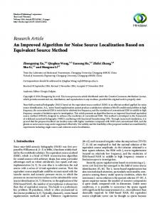
The simulation (with 100 ordinary nodes) results are shown by the Figure2. 7 LSM LSM-DS

6

A. The Analysis of Derivation Process According to expressions in part IV, when the error appears, the (4) and (5) are changed to (8) and (9). (8) AX = B * + E . T −1 T * (9) X = ( A A) A ( B + E ) . where B = B* + E .

And the (10) can be transformed to (10).

X = ( AT A) −1 AT B + ( AT A) −1 AT E .

(10) In order to expound clearly, we suppose the fellows:

F = ( AT A) −1 AT . Then, we can get:

X = F ( B + E ) = X * + FE

5

4

And both sides are computed the Euclidean norm, we can get:

3

X − X*

= FE 2 .

2

By using Cauchy-Schwarz inequality, the following inequality can be obtained.

2

1

0 0

.

X − X * = FE

FE 2 = 10

20

30

40

50

60

70

80

90

n

n

∑ ∑a i =1 k =1

100

Figure2. Comparing the error between LSM and LSM_DS

≤



n

i =1

Comparing the errors between LSM and LSM_DS, we get the results are shown in Figure.2. The ordinate represents the error; the abscissa represents the number of nodes; the solid line represents the error curve of LSM, and the dashed line represents the error curve of LSM_DS. We can see from the Figure2 that the LSM_DS algorithm only improves a part of the precision, but the


n

∑ (∑ a k =1

ik

n

n

i =1

k =1

∑ (∑ a

e ≤

ik k

2

ik

ek ) 2

n 2  )(∑ ek ) k =1 

.

= F F E2 Based on the above conclusion, we can get: X − X * = FE 2 ≤ F F ⋅ E 2 . 2

When the Euclidean norm of error vector E is the minimum, the Euclidean norm of vector FE can be smaller, that is to say:


113

X − X* ∝ E 2. 2

Because the Euclidean norm of vector (X-X*) equals that of EF, and the Euclidean norm of vector (X-X*) can be transformed to (11).

x  x  =   −  *  y   y  *

X − X*

2

x − x  =  *  y − y  2 .

In the measuring range, the impact factor caused by the distance measurement errors can be approximately set to the same value, so let γ i = γ j = γ . Equation (14) can be transformed to (15).

2 ei' = ( − 1)(ei2 − e 2j ) .

*

2

(11)

And the error vector can be got.

e12 − e 2j   2  E = ( )  ...  . γ  2 2 en − e j 

= (x − x ) + ( y − y ) * 2

* 2

According to (11), the Euclidean norm of vector (X- X*) is just the error between the calculating value of the node and the real value of it. Based on the above proof, the lower the error measurement is, the higher the recognition precision can be got. So a theorem can be given. Theorem 1: If the Euclidean norm of E is the smallest, the error between the calculating value of the node and the real value of it can be lower. So the problem is transformed to find an anchor node, the measurement error of which can make the Euclidean norm of E be the minimum. In (7), when the equation of benchmark node minus the equation of other nodes, the right expression of (7) is:

( x12 − x 2j ) + ( y12 − y 2j ) + (d1 + e1 ) 2 − (d j + e j ) 2   2  2 2 2 2 2 ( x2 − x j ) + ( y2 − y j ) + (d 2 + e2 ) − (d j + e j )  . B=  ....   ( x 2 − x 2 ) + ( y 2 − y 2 ) + ( d + e ) 2 − ( d + e ) 2  j n j n n j j  n  In order to discourse clearly, let the following expression be: bi = ( xi2 − x 2j ) + ( yi2 − y 2j ) + (d i2 − d 2j ) i = 1,2,3..., n .  ' 2 2 ei = (2d i ei − 2d j e j ) + (ei − e j ) So the B can be transformed to (13).

c1 + (2d1e1 − 2d j e j ) + (e12 − e 2j )    2 2 c2 + (2d 2e2 − 2d j e j ) + (e2 − e j )  . B=  ....   c + ( 2 d e − 2 d e ) + (e 2 − e 2 )  n n j j n j   n

(13)

B = B* + E .

e1'  c1    B * = ...  , E = ...  . e '  cn   n As we know, measurement error is proportional to the distance, and let ei = γ i d i .

γi

=(

2

γi

2

γj

e 2j ) + (ei2 − e 2j )

− 1)e − ( 2 i


.

2

γj

− 1)e

e12 − e 2j   2  = ( )  ...  γ  2 2 en − e j 

2 j

.

(16)

2 n = ( )∑ (ei2 − e 2j ) 2

γ

i =1

And both the right and left of (16) are squared.

(E )

2

(

E2∝ E

2 n = ( )∑ (ei2 − e 2j ) 2 .

γ

)

2

2

i =1

n

∝ J = ∑ ek2 − e 2j . i =1

B. Algorithm process • Step1: Find the all anchor nodes in the perception of distance • Step2: For each anchor node, compute its distance from the rest nodes, and get its J i .

J i , i = 1,2...n

and its corresponding node is the benchmark node. • Step4: Degree reduction. • Step5: Refinement using the least square algorithm. We choose the anchor node with minimum related distance as benchmark anchor node. In the LSM_DR algorithm, the anchor node which has the smallest J i is chosen to be the benchmark node, and the simulation is shown by the Figure3.

So the (12) can be transformed to (14).

ei2 −

2

• Step3: Choose the minimum from

where

2

E

e12 − e 2j   2  = ( )  ...  γ  2 2 en − e j 

According to the Theorem 1, only if the Euclidean norm of E can be the smallest, Node identification accuracy will be higher.

Let

ei' = (

Because:

2

(12)

(15)

γ

(14)

114


-

5

As shown in table I, we can see that the average error of LSM_DR is the smallest among the three algorithms; the simulation has proved that the LSM_DR can obtain more accurate localization while making the algorithm concise.

4

VII. CONCLUSIONS

7 LSM LSM- DR

6

3

2

1

0 0

10

20

30

40

50

60

70

80

90

100

Figure3. Comparing the error between LSM and LS_DR.

In Firure3, the ordinate represents the error; the abscissa represents the number of nodes; the red solid line represents the error curve of LSM; the dashed line represents the error curve of LSM_DR. As shown in Figure3, we can see that the majority of nodes’ localization error is reduced. VI. SIMULATION By using random deployed 100 ordinary nodes with seven anchor nodes around them, the distances between the ordinary node and the anchor nodes are unequal and disproportionate, the distance error is a random positive number and it is less than the 30% of the distance. The simulation by using LSM, LSM_DS and LSM_DR about localization is shown as the Figure4 and the Table1. 7

LSM LSM- DS

6

LSM- DR 5

4

3

2

1

0 0

10

20

30

40

50

60

70

80

90

100

Figure4. Comparing the errors among LSM, LS_DS and LS_DR.

As shown in Figure4, the ordinate represents the error; the abscissa represents the number of nodes; the red solid line represents the error curve of LSM; the dashed line represents the error curve of LSM_DS; the dotted line represents the error curve of LSM_DR. TABLE I. THE ERRORS OF THE THREE METHODS Algorithm

LSM

Average error

1.4044


LSM_DS 1.7691

LSM_DR 0.9784

This paper aims at improving the localization precision of nodes when using the least squares algorithm in WSN. Firstly the paper analyses the reasons why the extra error exists when subtracting the equation of distance between the anchor nodes and the ordinary nodes from the others in the LSM algorithm, and then proposes the principle of choosing the benchmark anchor nodes by using the distance’ errors of the benchmark anchor nodes in order to reduce the errors. The localization errors of these three algorithms are compared by using simulation in MATLAB, the result shows that the coordinator’s errors of the nodes decrease, and the improved algorithm proposed in this paper can effectively improve the precision of the nodes localization. ACKNOWLEDGMENT This research was supported by the Research and Development Project of Science and Technology of Yichang (Grant No.A2011-302-14); the National Natural Science Foundation of China (Grant No. 60972162);the National Natural Science Foundation of China (Grant No.41172298). REFERENCES [1] K. Lorincz, D. Malan, T.R.F. Fulford-Jones, A. Nawoj, A. Clavel, V.Shnayder, G. Mainland, M. Welsh, S. Moulton, Sensor networks for emergency response: challenges and opportunities, Pervasive Computing for First Response (Special Issue), IEEE Pervasive Computing ,2004. [2] T. Gao, D. Greenspan, M. Welsh, R.R. Juang, A. Alm, Vital signs monitoring and patient tracking over a wireless network, Proceedings of the 27th IEEE EMBS Annual International Conference, 2005. [3] G. Wener-Allen, K. Lorincz, M. Ruiz, O. Marcillo, J. Johnson, J. Lees, and M. Walsh, Deploying a wireless sensor network on an active volcano. Data-Driven Applications in Sensor Networks (Special Issue), IEEE Internet Computing, 2006. [4] He T, Huang CD, Blum B.M, range-free localization schemes in large scale sensor networks, Proc of the 9th Annual Int’l Conf on Mobile Computing and Networking. San Diego: ACM Press, 2003:81-95. [5] Qun, Wan, Wanlin, Yang, A fast algorithm for wireless sensor networks localization based on metric least squares scaling, IET International Conference on Wireless Mobile and Multimedia Networks Proceedings, ICWMMN 2006. [6] Born, Alexander; Timmermann, Dirk; Bill, Ralf A distributed linear least squares method for precise localization with low complexity in wireless sensor networks Distributed Computing in Sensor Systems Second IEEE International Conference, DCOSS 2006, Proceedings. [7] Zenon Chaczko, Ryszard Klempous, Jan Nikodem, Michal Nikodem, Methods of Sensors Localization in Wireless Sensor Networks, Proceedings of the 14th Annual IEEE


[8]

[9]

[10]

[11]

[12]

[13]

[14]

[15]

[16]

International Conference and Workshops on the Engineering of Computer-Based Systems (ECBS07), 2007. Savarese C, Rabaey JM, Beutel J, Localization in distributed ad-hoc wireless sensor network, Proceeding of the 2001 IEEE International Conference on Acoustics, Speech, and Signal Salt Lake, 2001. Avvides A, Park H, Srivastava M.B, The bits AND flops of the N-hop multilateration primitive for node localization problems, Proceeding of the 1st ACM International Workshop on Wireless Sensor Networks and Applications, Atlanta, 2002. Savarese C, Rabaey JM, Langendoen K, Robust Localization Algorithms for Distributed Ad Hoc Wireless Sensor Networks, Proceedings of the USENIX Technical Annual Conference, Monterey, USA, 2002. Bergamo P, Mazzini G.: Localization in sensor networks with fading and mobility. Processing of the 13th IEEE International Symposium on Personal, Indoor and Mobile Radio Communications, NJ, USA, 2002. Guha S, Murty R N, Sirer E G, A unified node and event localization framework using non-convex constraints, Proceeding of the 6th ACM International Symposium on Mobile Ad Hoc Networking and Computing, IL USA, 2005. Cao M, Anderson B D O, Morse A.S, Sensor network localization with imprecise distances, Systems and Control Letters, 2006. Srirangarajan S, Tewfik A H, Luo Z Q, Distributed sensor network localization with inaccurate anchor positions and noisy distance information. IEEE International Conference on Acoustics, Speech and Signal Processing, HI, USA, 2007. Xiaohui Chen, Jing He, Jinpeng Chen, An Improved Localization Algorithm for Wireless Sensor Network, Intelligent Automation and Soft Computing, Vol. 17, No. 5, pp. 507-517, 2011. Xiaohui Chen, Jing He, Jinpeng Chen, Localization of Node in Wireless Sensor Network Based on Conjugate Algorithm, 2011 International Conference on Computer Science and Service System, 2011.


115

Xiaohui Chen was born in Sichuan province, China in 1967, he received his master’s degree from Huazhong University of Science and Technology (HUST) , Wuhan, China, in 1996, He is currently an associate professor in the college of computer and information technology, China Three Gorges University. His research interests include wireless sensor networks, data mining, and intelligent control. Jing He was born in Hubei province, China in 1987, he received his bachelor's degree from Huazhong University of Science and Technology (HUST) , Wuhan, China,in 2010, and he is seeking for his master’s degree in the college of computer and information technology , China Three Gorges University now. His research fields include wireless sensor networks, embedded system. Bangjun Lei was born in 1973. he got his Ph.D title from TUDelft, the Netherlands In 2003. He is professor at the College of Computer and Information Technology, China Three Gorges University. He is active in low-level image processing, 3-D imaging and computer vision. He enjoys developing practical multimedia applications. Tingyao Jiang was born in 1969. He received the Ph.D. degree in College of Computer Science and Technology, Huazhong University of Science and Technology, Wuhan, China, in 2004. He is a professor in the College of Computer and Information Technology, China Three Gorges University. His research interests include fault-tolerant computing, network security, software engineer.