Hindawi Publishing Corporation Journal of Applied Mathematics Volume 2013, Article ID 734020, 9 pages http://dx.doi.org/10.1155/2013/734020
Research Article An Inverse Problem of Temperature Optimization in Hyperthermia by Controlling the Overall Heat Transfer Coefficient Seyed Ali Aghayan,1 Dariush Sardari,1 Seyed Rabii Mahdi Mahdavi,2 and Mohammad Hasan Zahmatkesh3 1
Faculty of Engineering, Science and Research Branch, Islamic Azad University, P.O. Box 14515-775, Tehran, Iran Medical Physics, Tehran University of Medical Science, Tehran, Iran 3 Medical Physics, Shahid Beheshti University, Tehran, Iran 2
Correspondence should be addressed to Seyed Ali Aghayan; ali
[email protected] Received 14 January 2013; Revised 1 July 2013; Accepted 8 July 2013 Academic Editor: Tin-Tai Chow Copyright © 2013 Seyed Ali Aghayan et al. This is an open access article distributed under the Creative Commons Attribution License, which permits unrestricted use, distribution, and reproduction in any medium, provided the original work is properly cited. A novel scheme to obtain the optimum tissue heating condition during hyperthermia treatment is proposed. To do this, the effect of the controllable overall heat transfer coefficient of the cooling system is investigated. An inverse problem by a conjugated gradient with adjoint equation is used in our model. We apply the finite difference time domain method to numerically solve the tissue temperature distribution using Pennes bioheat transfer equation. In order to provide a quantitative measurement of errors, convergence history of the method and root mean square of errors are also calculated. The effects of heat convection coefficient of water and thermal conductivity of casing layer on the control parameter are also discussed separately.
1. Introduction Hyperthermia treatment is recognized as an adjunct cancer therapy technique following surgery, chemotherapy, and radiation techniques. In hyperthermia, the tumor cells will be overheated, typically 40–45∘ C, to damage or kill the cancer cells [1, 2]. The determination of temperature distribution throughout the biological tissue by solving the simple Pennes bioheat Equation (Eq) and increment of tumor temperature to therapeutic value avoiding the overheating of the healthy tissue are important issues of investigation in hyperthermia [3]. Because of obvious reasons, which are not going to be discussed here, the water (or any other dielectric liquid) bolus is known as a necessary element of all contact applicators used in clinics in order to provide local heating of malignant tumors by means of electromagnetic (EM) energy [4]. There are numerous papers discussing the effect of the water coupling bolus on the temperature of surface and tissue specific absorption rate (SAR) during hyperthermia treatment [5, 6]. Sherar et al. [7] presented a new way to design the water
bolus for external microwave applicators which increased the available treatment field size by removing the central hotspot caused by the increased power from the applicator in this region. They also used beam shaping bolus with an array of saline-filled patches inside the coupling water bolus for superficial microwave hyperthermia [8]. Ebrahimi-Ganjeh and Attari [9] numerically computed and compared both the SAR distributions and effective field size in the presence and absence of water bolus. Neuman et al. [10] examined the effect of the various thickness of water bolus coupling layers on the SAR patterns from dual concentric conductor based on the conformal microwave array superficial hyperthermia applicators. One aspect of our investigation is optimal control theory, which is defined as a mathematical approach of manipulating the parameters affecting the behaviour of a system to produce the desired or optimal outcome. A recent development in this field is the optimal control of systems with distributed parameters which especially include the biological tissue in course of the hyperthermia treatment planning [11]. Butkovasky [11]
2 I
II
Casing layer a
0
2.1. Governing Equations and Model Geometry. Schematic diagram of the studied control zone is shown in Figure 1. In order to simplify demonstrating the methodology, heat transfer model is assumed to be one-dimensional. It should be noted that although we could develop a model with an irregular shape of a tumor embedded in the healthy tissue,
X
Figure 1: Schematic diagram of control zone. Cooling system consists of water bolus embedded in a casing layer which is placed between the applicator and biomedia. Regions I and II represent the healthy tissue and tumor region, respectively.
a homogeneous slab of tissue, including the tumor region, is considered. Temperature distribution inside the tissue could be obtained by solving the Pennes bioheat equation [19] as follows: 𝜌𝑡 𝑐𝑡
𝜕𝑇𝑡 (𝑥, 𝑡) = ∇ (𝑘𝑡 ∇𝑇𝑡 (𝑥, 𝑡)) + 𝜔bl 𝜌bl 𝑐bl (𝑇𝑎 − 𝑇𝑡 (𝑥, 𝑡)) 𝜕𝑡 + 𝑄𝑚 + 𝑄𝑟 (𝑥, 𝑡)
0 < 𝑥 < 𝑎, (1)
𝑇𝑡 (𝑥, 𝑡) = 𝑇𝑐 −𝑘𝑡
𝑥 = 0,
𝜕𝑇𝑡 (𝑥, 𝑡) = 𝑈 (𝑇∞ − 𝑇𝑡 (𝑥, 𝑡)) 𝜕𝑥 𝑇𝑡 (𝑥, 𝑡) = 𝑇𝑖
(2) 𝑥 = 𝑎,
0 < 𝑥 < 𝑎 , 𝑡 = 0,
(3) (4)
where 𝑈 is the overall heat transfer coefficient, which defines the effectiveness of the cooling system. Because the temperature distribution is very sensitive to the heat transfer between the cooling liquid and the so-called tissue, its numerical value must be properly estimated. It is shown that the expression of 𝑈 is [20] as follows: 𝑈=
2. Optimization Scheme
Water bolus
I
Radiating antenna
treated the fundamentals in the theory of optimal control of systems with distributed parameters. Wagter [12] studied an optimization procedure to calculate the transient temperature profiles in a plane tissue by multiple EM applicators. Kuznetsov [13] used the minimum principle of Pontryagin to solve an optimum control problem for heating a layer of tissue in order to destroy a cancerous tumor. Although the Levenberg-Marquardt and simplex methods are common techniques for solving optimization problems, we tend to develop a methodology to numerically optimize hyperthermia treatments based on an inverse heat conduction problem by using the conjugate gradient method with an adjoint equation (CGMAE). One of the advantages of the CGMAE is its insensitivity to initial variables; however, it requires a numerical method for each iteration to determine the temperature fields, which involves computing the gradients of objective function. In the last two decades, CGMAE has been widely used in the solution of the general inverse heat transfer problems (IHTPs) regarding the optimization procedure [14] especially in therapeutic applications [15–17]. The most common approach for determining the optimal estimation of the model parameters, functions, or boundary conditions is to minimize an objective function. In this study, the objective function to be minimized is based on the criterion of minimal square root of the difference between the desired temperature and the computed one. We demonstrate that optimum heating conditions inside the biological tissue, which is caused by an applied radiofrequency (RF) heat source, can be numerically attained within the total time of the process by means of controlling the overall heat transfer coefficient associated with the cooling system. To do this and to reach the appropriate configuration of cooling system, thermal properties of water bolus and casing layer are considered as variable parameters. Recently, few studies have been conducted with the aim of beam-forming in hyperthermia which are based on utilizing the saline patches inserted in the cooling system or the solid absorbing blocks between the applicator and water bolus [7, 8, 18]. However, best to our knowledge, none of them has used an inverse model to control the thermal or electrical properties of these additional patches or blocks. In the perspective of the model, we believe that the desired temperature profile inside the tumor according to its shape and size can be achieved by inversely optimizing the shape, thickness, electrical, and thermal properties of solid or liquid patches which are inserted in the cooling system. Therefore, the proposed algorithm developed in this study could be effectively used by physicians to design an optimal treatment plan in a large variety of therapeutic treatments.
Journal of Applied Mathematics
1 . 1/ℎ + l/𝑘cl
(5)
Here, ℎ is the heat convection coefficient of water and 𝑙 and 𝑘cl are the thickness and thermal conductivity of the casing layer, respectively. For the inverse problem proposed here, the overall heat transfer coefficient of cooling system is considered as an unknown function, while the other quantities within the formulation of the direct problem presented previously are
Journal of Applied Mathematics
3
assumed to be known precisely. Moreover, the temperature distribution inside the tissue region is considered available. The optimization procedure includes maximizing the temperature inside the tumor while minimizing it in the normal surrounding tissue via a proposed objective function. In other words, we tend to achieve the desired temperature, 𝑌𝑡 (𝑥𝑗 , 𝑡), at 𝑁 points whether in the tumor region or in the healthy one, by optimal control of 𝑈 within the total time 𝑡𝑓 of the treatment process. Therefore, the following function must be minimized: 𝑁
𝑡𝑓
2
𝐺 (𝑈) = ∑ ∫ [𝑇𝑡 (𝑥𝑗 , 𝑡, 𝑈) − 𝑌𝑡 (𝑥𝑗 , 𝑡)] 𝑑𝑡, 𝑗=1 0
The iterative procedure of CGMAE for the optimization of 𝑈 is given by 𝑈𝑙+1 = 𝑈𝑙 − 𝛽𝑙 𝑑𝑙
Here, 𝛽𝑙 is the step size and 𝑑𝑙 is the descent direction of the 𝑙th iteration which is defined as follows: 𝑑𝑙 = ∇𝐺𝑙 + 𝛾𝑙 𝑑𝑙−1
(6)
𝑑0 = 0.
2 ∇𝐺 (𝑈𝑙 ) 𝛾 = ∇𝐺 (𝑈𝑙−1 )2 𝑙
(11)
𝛾0 = 0.
(12)
Then, the step size could be derived from the following equation: 𝑡
𝐿 (𝑇𝑡 , Ψ𝑡 , 𝑈) = 𝐺 (𝑈)
𝑙
𝛽 =
𝑡𝑓
𝑎
0
0
+ ∫ ∫ Ψ𝑡 (𝑥, 𝑡) [𝑘𝑡
2
𝜕 𝑇𝑡 (𝑥, 𝑡) 𝜕𝑥2
− 𝜌𝑡 𝑐𝑡
𝜕𝑇𝑡 (𝑥, 𝑡) 𝜕𝑡
+ 𝜔bl 𝜌bl 𝑐bl (𝑇𝑎 − 𝑇𝑡 (𝑥, 𝑡)) +𝑄𝑚 + 𝑄𝑟 (𝑥, 𝑡) ] 𝑑𝑥 𝑑𝑡,
𝑓 ∑𝑁 𝑗=1 ∫0 {𝑇𝑡 (𝑥𝑗 , 𝑡) − 𝑌𝑡 (𝑥𝑗 , 𝑡)} Δ𝑇𝑡 (𝑥𝑗 , 𝑡) 𝑑𝑡
where Ψ𝑡 (𝑥, 𝑡) is the Lagrange multiplier obtained by solving the adjoint problem which is defined by the following set of equations: 𝜕2 Ψ𝑡 (𝑥, 𝑡) 𝜕Ψ (𝑥, 𝑡) + 𝜌𝑡 𝑐𝑡 𝑡 − 𝜔bl 𝜌bl 𝑐bl Ψ𝑡 (𝑥, 𝑡) 𝜕𝑥2 𝜕𝑡
Ψ𝑡 (𝑥, 𝑡) = 0
Here, Δ𝑇𝑡 (𝑥𝑗 , 𝑡) is the answer to the sensitivity problem. As mentioned in the appendix, we present the methodology used to analytically derive the sensitivity, the adjoint problems, and the gradient equation. The iteration procedure is repeated until it satisfies the following truncation criteria and then leads to optimal control of the overall heat transfer coefficient as follows: 𝑈𝑙+1 − 𝑈𝑙 ≤ 𝑒, 𝑈𝑙
(8)
where 𝑒 is a small number (10−4 ∼10−5 ). The computational algorithm for the foregoing procedure is given by the following.
(4) Solve the adjoint problem. (5) Compute the gradient equation. (6) Compute the conjugate coefficient 𝛾𝑙 and the direction of descent 𝑑𝑙 .
𝑥 = 𝑎,
(7) Solve the sensitivity problem.
where 𝛿 is the Dirac function. Adjoint problem can also be solved by the same method as the direct problem of (1), that is, by using the finite difference time domain method (FDTD). It can be shown that the gradient of residual functional, ∇𝐺, could be expressed by the following analytical expression: ∇𝐺 (𝑈) = ∫ Ψ𝑡 (𝑎, 𝑡) (𝑇𝑡 (𝑎, 𝑡) − 𝑇∞ ) 𝑑𝑡. 0
(14)
(3) Examine (14), and if convergence is satisfied, stop; otherwise, continue.
Ψ𝑡 (𝑥, 𝑡) = 0 0 < 𝑥 < 𝑎, 𝑡 = 𝑡𝑓 ,
𝑡𝑓
. (13)
(2) Solve the direct problem.
𝑥 = 0,
𝜕Ψ𝑡 (𝑥, 𝑡) = Ψ𝑡 (𝑥, 𝑡) 𝑈 𝜕𝑥
2
(1) Give an initial guess for 𝑈.
+ 2 [𝑇𝑡 (𝑥𝑗 , 𝑡) − 𝑌𝑡 (𝑥𝑗 , 𝑡)] × 𝛿 (𝑥 − 𝑥𝑗 ) = 0 0 < 𝑥 < 𝑎,
𝑡
𝑓 ∑𝑁 𝑗=1 ∫0 {Δ𝑇𝑡 (𝑥𝑗 , 𝑡)} 𝑑𝑡
(7)
𝑘𝑡
(10)
The coefficient of conjugate gradient, 𝛾𝑙 , is given by
where 𝑇𝑡 (𝑥𝑗 , 𝑡, 𝑈) is the computed temperature. In order to minimize 𝐺(𝑈) under the constraints mentioned in (1)–(4), we introduce a new function called the “Lagrangian function” (𝐿) which associates (6) and (1) with the following equation:
𝑘𝑡
𝑙 = 0, 1, 2, . . . .
(9)
(8) Compute the search step size 𝛽𝑙 . (9) Increment the controlling parameter using (10) and return to Step 1. 2.2. Model Parameters 2.2.1. Electromagnetic Model. The spatial and temporal behaviors of the EM field inside the tissues and are governed
4
Journal of Applied Mathematics
by Maxwell’s equations. In a homogeneous tissue, these equations are expressed by [21] the following: ∇ × 𝐸 = 𝑖𝜔𝜇𝐻, ∇ ⋅ 𝐸 = 0, ∇ ⋅ 𝐻 = 0,
Table 1: Biophysical characteristics of model. Component Blood
(15)
∇ × 𝐻 = −𝑖𝜔𝜀∗ 𝐸, where 𝐸 and 𝐻 are, respectively, complex electric and magnetic fields, 𝜔 is the angular frequency, and 𝜀, 𝜎 and 𝜇 are the electrical permittivity, the electrical conductivity, and the magnetic permeability of tissue, respectively. 𝜀∗ is the complex permittivity which is defined by 𝑖𝜎 (16) . 𝜔 The volumetric EM power deposition, which averaged over time, is calculated by 𝜀∗ = 𝜀 +
𝜎|𝐸|2 (17) , 𝑄𝑟 = 2 where |𝐸| is the root mean square magnitude [V/m] of the incident electric field in a point which could be calculated through (15). 2.2.2. Cooling System and Tissue Properties. Thermophysical properties of tissue and blood, pertaining to the model for numerical simulation, are provided in Table 1 [3, 22, 23]. The thickness of water is set at 10−2 m and the electrical permittivity and electrical conductivity of water, related to an RF applicator operating at 432 MHz, are 78 and 0.0300 S/m, respectively [23]. Moreover, thicknesses of 0.03 m and 1.5 × 10⁻⁴ m are used, respectively, for tissue and casing layer which are typically made of thin flexible Silicon layers. Temperature of the cooling system, 𝑇∞ , is set at 15∘ C.
3. Assumptions In order to simplify demonstrating the methodology, heat transfer is assumed to be one-dimensional with a constant rate of tissue metabolism and blood perfusion. The target temperatures, after the elapse of allowed heating period, are set between 42 and 45∘ C for tumoral region and 42∘ C or lower for normal tissues. In addition, we consider three different nodes: one in the tumor region with 𝑌(0.007, 𝑡𝑓 ) = 43∘ C and two others in the normal tissue with 𝑌(0.002, 𝑡𝑓 ) and 𝑌(0.021, 𝑡𝑓 ) = 39∘ C as the desired temperatures. As the thickness of the casing layer is much smaller than its wavelength, it could be neglected in the EM analysis. Moreover, the thermal contact between the casing layer and tissue is assumed to be perfect so that the thermal contact resistance between these layers is negligible.
4. Results and Discussions In the present work, FDTD method is used for numerical solution of the direct, sensitivity, and adjoint problems. A
Tissue
Parameter 𝑐bl 𝜌bl 𝜔bl 𝑐𝑡 𝑘𝑡 𝑄𝑚 𝑇𝑎 𝑇𝑐 𝑇𝑖 𝜀𝑡 𝜌𝑡 𝜎𝑡
Value 4200 1000 0.0005 3770 0.5 33800 37 37 34 55 998 1.1
Units j/kg ∘ C kg/m3 mL/s/mL j/kg ∘ C W/m ∘ C W/m3 ∘ C ∘ C ∘ C — kg/m3 S/m
uniform grid of 31 × 31 mesh in space and time is utilized for all the results presented hereafter. The optimization algorithm presented previously is programmed in Fortran 90, compiled through the software Compaq Visual Fortran Professional Edition on a computer with an Intel Core i7 3.5 GHz and 16 Gb of RAM. The final time, 𝑡𝑓 , is chosen equal to 1800 s. Moreover, the computational precision (𝑒) is set at 10−5 . In the following simulation, the desired temperature distribution is determined by precisely prescribing a known 𝑈. Figure 2 indicates the sensitivity of the temperaturetime curve for variations in 𝑈 for three different values of 𝑈. Because of the large values of the sensitivity with respect to 𝑈, obviously the proposed optimization model is “well-conditioned.” To illustrate the accuracy of the present inverse analysis, the initial approximations of 𝑈 were either increased or decreased from its known value. Figure 3 shows the number of convergent iterations with different initial guesses for 𝑈. Changing the initial value, for example, by 15% and 30% of its known value does not affect the solution and the optimization object is still satisfied. Moreover, it is clear that the number of convergent iterations is reduced when the initial guess value varies within a 15% deviation from the known one. In addition, this figure shows that the minimization of the objective function is valid when 𝑈 varies between 125 and 200 W/m2∘ C. In order to provide a quantitative measurement of errors, the convergence history of the presented model is also calculated. Figure 4 compares the convergence history is of three different initial guesses. Convergence history is measured by the relative error at each iteration, that is, |𝑈retrieved − 𝑈prescribed |/𝑈prescribed . The computed temperature distribution is obtained when the minimization of the objective function is satisfied, that is, when the optimal value of 𝑈 is achieved. Figure 5 shows the computed temperature distribution with initial guess of 𝑈 = 200 W/m2∘ C as well as the desired one, which is obtained from the application of a known 𝑈 at 𝑡 = 1000 s. It is observed that the recovered temperature distribution is in good agreement with the desired one. In addition, the computed RMS error is equal to 0.24. Figure 6 presents the desired temperature distributions result from the solution of
Journal of Applied Mathematics
5
0.7
10−0
0.6
10−1 Relative error
ΔT (∘ C)
0.5 0.4 0.3 0.2
10−2 10−3 10−4 10−5
0.1 0 0
0.1
0.2
0.3
0.4
U = 150 W/m2 ∘ C U = 175 W/m2 ∘ C U = 200 W/m2 ∘ C
0.5 t/tf
0.6
0.7
0.8
0.9
10−6
1
2
4
6
8
10 12 Iteration
14
16
18
20
Figure 4: Comparison of convergence histories of CGM for different initial guesses— ◊: 125, ◻: 150, and I: 200 W/m2∘ C for 𝑈.
Figure 2: Temperature sensitivity resulting from variations in 𝑈. I
43
II
I
Temperature (∘ C)
U (W/m2 ∘ C)
200
175
40
37
150 34 125 2
4
6
8 10 12 14 Number of iterations
16
18
0
0.01 0.02 Depth of tissue (m)
20
0.03
Prescribed temperature distribution Recovered temperature distribution
Figure 3: Convergence curve for different initial guesses of 𝑈.
Figure 5: A comparison between recovered and desired temperature distribution at 𝑡 = 1000 s.
43
Temperature (∘ C)
the nonstationary thermal problem during the total heating process. It is found to be sufficient to elevate the temperature inside the tumor to 42∘ C within approximately 20 minutes, while the temperature on the surface remains approximately constant in this period of time. According to the foregoing discussion, as (5), and in order to enhance the performance of the cooling system, the thermal conductivity of casing layer and the heat convection coefficient of water have been considered as variable parameters. Although the casing layer is very thin, as shown in Figure 7, the influence of thermal conductivity of casing layer is remarkable. It could be observed that a slight increase in thermal conductivity reduces significantly the temperature at the skin surface. In addition, the position of the maximum temperature is shifted slightly toward the skin. The second possibility to control the effectiveness of the cooling system is through the variation of the heat convection coefficient of water. Figure 8 indicates the influence of two different values of ℎ on the temperature of tissue. It could be observed that a 75% increase in ℎ results in a decrease of about 2.5∘ C in the skin and only 2∘ C in the maximum. The same results could be obtained by only 20% of the variation in the thermal
40
37
34
31 0
0.01 0.02 Depth of tissue (m) t= t= t= t=
200 s 500 s 600 s 1000 s
0.03
t = 1200 s t = 1600 s t = 1800 s
Figure 6: Transient spatial temperature distribution inside the tissue.
6
Journal of Applied Mathematics
40
such as 𝑈 = 𝑓(𝑦, 𝑧), it has the potential to provide a more comprehensive understanding of the cooling system ability for the purposes of beam-forming in two or three dimensions. This modified optimization algorithm is then implemented to the tumor and its surrounding tissue to determine the optimal properties of cooling system.
37
5. Conclusions
Temperature (∘ C)
43
34 0
0.01 0.02 Depth of tissue (m)
0.03
Figure 7: Temperature distribution at 𝑡 = 1000 s for two different thermal conductivities of casing layer. Solid line: 𝑘cl = 0.14 W/m∘ C, 𝑈 = 175 W/m2∘ C; dashed line: 𝑘cl = 0.11 W/m∘ C, 𝑈 = 150 W/m2∘ C.
Temperature (∘ C)
43
40
37
In this paper, we demonstrated the validity of the CGMAE in the optimization of the temperature distribution inside the tissue by optimal control of the overall heat transfer coefficient associated with the cooling system. The temperature distribution inside the tissue, based on the bioheat transfer equation, has also been numerically computed. In order to evaluate the effectiveness of the cooling system, the thermal conductivity of casing layer and the heat convection coefficient of water have been considered separately. According to results, the presented model allows obtaining the best properties of water and casing layer in the light of optimization and therefore significantly improves the treatment outcome. However, this method shows great promise for further extensions in both model and clinical performances for any shaped targeted tumor in hyperthermia treatments.
Appendix
34
31 0
0.01 0.02 Depth of tissue (m)
0.03
Figure 8: Temperature distribution at 𝑡 = 1000 s for two different heat convection coefficients of water. Solid line: ℎ = 200 W/m2∘ C,𝑈 = 175 W/m2∘ C; dashed line: ℎ = 350 W/m2∘ C, 𝑈 = 200 W/m2∘ C.
conductivity of casing layer. However, depending on the technical facilities, one can make an optimal decision in this case. Although the thickness and the electrical conductivity of water can also be optimized in the treatment process, we did not consider them in this study and we mainly focused on the influence of the overall heat transfer coefficient on the temperature field inside the tissue. In the perspective of the present model, we believe that the desired temperature profile inside the tumor, according to its shape and size, can be achieved by inversely optimizing the shape, thickness, electrical, and thermal properties of solid or liquid patches which are inserted in the cooling system. Such an optimization problem should also incorporate the best configuration of the additional patches which reasonably must resemble the tumor shape, for example, L-form patches for L-form tumors. However, the clinician will first scan the geometry of the tumor and measure the tumor size and depth using an MRI or CT or other noninvasive imaging techniques. Although the present model is based on the 1D heat transfer, but with some modifications in the governing formulations,
In order to find the minimum of the residual function by gradienttype method, it is required to derive its gradient by the following processes first, computation of the variation problem when the unknown has a small variation, and second, inspection of the conditions under which we obtain a stationary point for the Lagrange functional. To compute the variation problem, the unknown function 𝑈 is perturbed by Δ𝑈; that is, 𝑈𝜀 = 𝑈 + Δ𝑈.
(A.1)
Then, the temperature undergoes the variation Δ𝑇𝑡 (𝑥, 𝑡) as follows: 𝑇𝑡𝜀 (𝑥, 𝑡; 𝑈) = 𝑇𝑡 (𝑥, 𝑡; 𝑈) + Δ𝑇𝑡 (𝑥, 𝑡; 𝑈) ,
(A.2)
where 𝜀 refers to the perturbed variables. By inserting the a aforementioned equations in the direct problem and subtracting the original (1)–(4) from the resulting expressions and ignoring the second order terms, the following direct problem in variation is obtained: 𝜌𝑡 𝑐𝑡
𝜕Δ𝑇𝑡 (𝑥, 𝑡) 𝜕2 Δ𝑇𝑡 (𝑥, 𝑡) = 𝑘𝑡 𝜕𝑡 𝜕𝑥2 − 𝜔bl 𝜌bl 𝑐bl Δ𝑇𝑡 (𝑥, 𝑡)
(A.3) 0 < 𝑥 < 𝑎,
Δ𝑇𝑡 (𝑥, 𝑡) = 0 𝑥 = 0, −𝑘𝑡
(A.4)
𝜕Δ𝑇𝑡 (𝑥, 𝑡) = Δ𝑈 (𝑇∞ − 𝑇𝑡 (𝑥, 𝑡)) 𝜕𝑥 − 𝑈Δ𝑇𝑡 (𝑥, 𝑡)
(A.5)
𝑥 = 𝑎,
Δ𝑇𝑡 (𝑥, 𝑡) = 0 0 < 𝑥 < 𝑎, 𝑡 = 0.
(A.6)
Journal of Applied Mathematics
7
The second step is to calculate the variation of the objective function, Δ𝐺(𝑈), which is given by 𝑡𝑓
𝑎
0
0
Δ𝐺 (𝑈) = ∫ ∫ 2 Δ𝑇𝑡 (𝑥𝑗 , 𝑡) [𝑇𝑡 (𝑥𝑗 , 𝑡) −𝑌𝑡 (𝑥𝑗 , 𝑡)]
of the mathematical terms) the final form of (A.8) can be written as follows: Δ𝐿 = ∫
𝑡𝑓
𝑎
∫ [𝑘𝑡 0
0
𝜕2 Ψ𝑡 (𝑥, 𝑡) 𝜕Ψ (𝑥, 𝑡) + 𝜌𝑡 𝑐𝑡 𝑡 2 𝜕𝑥 𝜕𝑡
(A.7)
− 𝜔bl 𝜌bl 𝑐bl Ψ𝑡 (𝑥, 𝑡)
× 𝛿 (𝑥 − 𝑥𝑗 ) 𝑑𝑥 𝑑𝑡.
+ 2 [𝑇𝑡 (𝑥𝑗 , 𝑡) − 𝑌𝑡 (𝑥𝑗 , 𝑡)]
We obtain the variation of the augmented functional, Δ𝐿(𝑇, Ψ𝑡 , 𝑈), by considering the variation problem given by (A.3) and the variation of the objective function, (A.7), as follows: 𝑡𝑓
× 𝛿 (𝑥 − 𝑥𝑗 ) ] Δ𝑇𝑡 (𝑥, 𝑡) 𝑑𝑥 𝑑𝑡 𝑡𝑓
− ∫ 𝑘𝑡 Ψ𝑡 (0, 𝑡) 0
𝑎
Δ𝐿 = ∫ ∫ 2 Δ𝑇𝑡 (𝑥𝑗 , 𝑡) [𝑇𝑡 (𝑥𝑗 , 𝑡) − 𝑌𝑡 (𝑥𝑗 , 𝑡)]
𝑡𝑓
0
0
𝑎
0
0
+ ∫ ∫ Ψ𝑡 (𝑥, 𝑡) [𝑘𝑡
0
𝑎
− ∫ 𝜌𝑡 𝑐𝑡 Ψ𝑡 (𝑥, 𝑡𝑓 ) Δ𝑇𝑡 (𝑥, 𝑡𝑓 ) 𝑑𝑥
2
𝜕 Δ𝑇𝑡 (𝑥, 𝑡) 𝜕𝑥2 − 𝜌𝑡 𝑐𝑡
0
𝑡𝑓
+ ∫ Δ𝑈 Ψ𝑡 (𝑎, 𝑡) (𝑇𝑡 (𝑎, 𝑡) − 𝑇∞ ) 𝑑𝑡.
𝜕Δ𝑇𝑡 (𝑥, 𝑡) 𝜕𝑡
0
−𝜔bl 𝜌bl 𝑐bl Δ𝑇𝑡 (𝑥, 𝑡) ] 𝑑𝑥 𝑑𝑡. (A.8)
(A.11)
To satisfy the optimality condition, that is, Δ𝐿(Δ𝑇, Ψ𝑡 , Δ𝑈) = 0, it is required that all coefficients of Δ𝑇𝑡 (𝑥, 𝑡) are to be vanished. Finally, the following term is left: 𝑡𝑓
Using integration by parts in (A.8),
Δ𝐿 (𝑇, Ψ𝑡 , 𝑈) = ∫ Δ𝑈 Ψ𝑡 (𝑎, 𝑡) (𝑇𝑡 (𝑎, 𝑡) − 𝑇∞ ) 𝑑𝑡. 0
𝜕2 Δ𝑇𝑡 (𝑥, 𝑡) Ψ𝑡 (𝑥, 𝑡) 𝑑𝑥 𝑑𝑡 ∫ ∫ 𝜕𝑥2 0 0 𝑡𝑓
𝜕Ψ𝑡 (𝑎, 𝑡) ) Δ𝑇𝑡 (𝑎, 𝑡) 𝑑𝑡 𝜕𝑥
+ ∫ (Ψ𝑡 (𝑎, 𝑡) 𝑈 − 𝑘𝑡
× 𝛿 (𝑥 − 𝑥𝑗 ) 𝑑𝑥 𝑑𝑡 𝑡𝑓
𝜕Δ𝑇𝑡 (0, 𝑡) 𝑑𝑡 𝜕𝑥
(A.12)
𝑎
𝑡𝑓
𝜕Ψ (𝑎, 𝑡) 𝜕Δ𝑇𝑡 (𝑎, 𝑡) Ψ𝑡 (𝑎, 𝑡) − 𝑡 Δ𝑇𝑡 (𝑎, 𝑡) 𝜕𝑥 𝜕𝑥
=∫ [ 0
𝑎
𝑡𝑓
0
0
𝐿 (𝑇, Ψ𝑡 , 𝑈) = 𝐺 (𝑈) ,
(A.13)
Δ𝐿 (𝑇, Ψ𝑡 , 𝑈) = Δ𝐺 (𝑈) .
(A.14)
−
𝜕Δ𝑇𝑡 (0, 𝑡) Ψ𝑡 (0, 𝑡) 𝜕𝑥
and then
+
𝜕Ψ𝑡 (0, 𝑡) Δ𝑇𝑡 (0, 𝑡)] 𝑑𝑡 𝜕𝑥
Based on the definition, the variation of the functional 𝐺(𝑈) can be written as follows:
𝑡𝑓
𝑎
0
0
+∫ ∫
∫ ∫
Since we know that 𝑇𝑡 (𝑥, 𝑡) and Ψ𝑡 (𝑥, 𝑡) are, respectively, the direct and the adjoint problem solutions, it follows that
𝜕2 Ψ𝑡 (𝑥, 𝑡) Δ𝑇𝑡 (𝑥, 𝑡) 𝑑𝑥 𝑑𝑡, 𝜕𝑥2
Δ𝐺 (𝑈) = ⟨∇𝐺, Δ𝑈⟩ , (A.9)
𝜕Δ𝑇𝑡 (𝑥, 𝑡) Ψ𝑡 (𝑥, 𝑡) 𝑑𝑡 𝑑𝑥 𝜕𝑡
where the associated inner scalar product ⟨, ⟩ of two functions 𝑓(𝑡) and 𝑔(𝑡) in the Hilbert space of 𝐿 2 (0, 𝑡𝑓 ) is defined by 𝑑
⟨𝑓 (𝑡) , 𝑔 (𝑡)⟩𝐿 2 = ∫ 𝑓 (𝑡) 𝑔 (𝑡) 𝑑𝑡. 𝑐
𝑎
= ∫ [Δ𝑇𝑡 (𝑥, 𝑡𝑓 ) Ψ𝑡 (𝑥, 𝑡) − Δ𝑇𝑡 (𝑥, 0) Ψ𝑡 (𝑥, 0)] 𝑑𝑥 0
𝑎
𝑡𝑓
0
0
− ∫ ∫
Δ𝑇𝑡 (𝑥, 𝑡)
𝜕Ψ𝑡 (𝑥, 𝑡) 𝑑𝑡 𝑑𝑥, 𝜕𝑥
(A.10)
and by using the boundary conditions of the direct problem in variations (Equations (A.3)–(A.6) and the rearrangement
(A.15)
(A.16)
From the definition of the scalar product, the variation of the functional 𝐺(𝑈) can be written as follows: Δ𝐺 (𝑈) = ⟨∇𝐺 (𝑈) , Δ𝑈⟩𝐿 2 = ∇𝐺 (𝑈) Δ𝑈.
(A.17)
A comparison between (A.12), (A.14), and (A.17) reveals that the gradient of the residual functional is given by (9). More details about the derivation of the equations are mentioned in [24–26].
8
Journal of Applied Mathematics
Nomenclature 𝑐: 𝑑: 𝑒: 𝐸: 𝐺(𝑈): Δ𝐺(𝑈): ∇𝐺(𝑈): ℎ: 𝐻: 𝑘: 𝑙: 𝐿: 𝑁: 𝑄𝑚 : 𝑄𝑟 : 𝑇: 𝑡: 𝑈: 𝑥: 𝑌:
Heat capacity Vector of descent direction Computational precision Complex electric field Residual functional Residual functional variation Gradient of residual functional Heat convection coefficient Complex magnetic field Thermal conductivity Thickness of casing layer Lagrangian functional Number of nodes Tissue metabolism Volumetric heat source Temperature Time Overall heat transfer coefficient Space Desired temperature.
Greek Symbols 𝛽: 𝛾: 𝛿: 𝜀: 𝜌: 𝜇: 𝜎: Ψ: 𝜔: 𝜔:
Descent parameter Descent direction parameter Dirac function Electrical permeability Density Magnetic permeability Electrical conductivity Lagrange multiplier Angular frequency Blood perfusion.
Subscripts 𝑎: bl: 𝑐: cl: 𝑓: 𝑖: 𝑡: ∞:
Arterial Blood Core Casing layer Final Initial time Tissue Ambient.
Superscripts 𝑙: Iteration number.
References [1] S. R. H. Davidson and D. F. James, “Drilling in bone: modeling heat generation and temperature distribution,” Journal of Biomechanical Engineering, vol. 125, no. 3, pp. 305–314, 2003. [2] W. G. Sawyer, M. A. Hamilton, B. J. Fregly, and S. A. Banks, “Temperature modeling in a total knee joint replacement using patient-specific kinematics,” Tribology Letters, vol. 15, no. 4, pp. 343–351, 2003.
[3] R. Dhar, P. Dhar, and R. Dhar, “Problem on optimal distribution of induced microwave by heating probe at the tumor site in hyperthermia,” Advanced Modeling and Optimization, vol. 13, no. 1, pp. 39–48, 2011. [4] E. A. Gelvich and V. N. Mazokhin, “Resonance effects in applicator water boluses and their influence on SAR distribution patterns,” International Journal of Hyperthermia, vol. 16, no. 2, pp. 113–128, 2000. [5] M. de Bruijne, T. Samaras, J. F. Bakker, and G. C. van Rhoon, “Effects of waterbolus size, shape and configuration on the SAR distribution pattern of the Lucite cone applicator,” International Journal of Hyperthermia, vol. 22, no. 1, pp. 15–28, 2006. [6] E. R. Lee, D. S. Kapp, A. W. Lohrbach, and J. L. Sokol, “Influence of water bolus temperature on measured skin surface and intradermal temperatures,” International Journal of Hyperthermia, vol. 10, no. 1, pp. 59–72, 1994. [7] M. D. Sherar, F. F. Liu, D. J. Newcombe et al., “Beam shaping for microwave waveguide hyperthermia applicators,” International Journal of Radiation Oncology Biology Physics, vol. 25, no. 5, pp. 849–857, 1993. [8] J. C. Kumaradas and M. D. Sherar, “Optimization of a beam shaping bolus for superficial microwave hyperthermia waveguide applicators using a finite element method,” Physics in Medicine and Biology, vol. 48, no. 1, pp. 1–18, 2003. [9] M. A. Ebrahimi-Ganjeh and A. R. Attari, “Study of water bolus effect on SAR penetration depth and effective field size for local hyperthermia,” Progress in Electromagnetics Research B, vol. 4, pp. 273–283, 2008. [10] D. G. Neuman, P. R. Stauffer, S. Jacobsen, and F. Rossetto, “SAR pattern perturbations from resonance effects in water bolus layers used with superficial microwave hyperthermia applicators,” International Journal of Hyperthermia, vol. 18, no. 3, pp. 180–193, 2002. [11] A. G. Butkovasky, Distributed Control System, American Elsevier, New York, NY, USA, 1969. [12] C. De Wagter, “Optimization of simulated two-dimensional temperature distributions induced by multiple electromagnetic applicators,” IEEE Transactions on Microwave Theory and Techniques, vol. 34, no. 5, pp. 589–596, 1986. [13] A. V. Kuznetsov, “Optimization problems for bioheat equation,” International Communications in Heat and Mass Transfer, vol. 33, no. 5, pp. 537–543, 2006. [14] C. Huang and S. Wang, “A three-dimensional inverse heat conduction problem in estimating surface heat flux by conjugate gradient method,” International Journal of Heat and Mass Transfer, vol. 42, no. 18, pp. 3387–3403, 1999. [15] P. K. Dhar and D. K. Sinha, “Temperature control of tissue by transient-induced-microwaves,” International Journal of Systems Science, vol. 19, no. 10, pp. 2051–2055, 1988. [16] T. Loulou and E. P. Scott, “Thermal dose optimization in hyperthermia treatments by using the conjugate gradient method,” Numerical Heat Transfer A, vol. 42, no. 7, pp. 661–683, 2002. [17] T. Loulou and E. P. Scott, “An inverse heat conduction problem with heat flux measurements,” International Journal for Numerical Methods in Engineering, vol. 67, no. 11, pp. 1587–1616, 2006. [18] H. Kroeze, M. Van Vulpen, A. A. C. De Leeuw, J. B. Van De Kamer, and J. J. W. Lagendijk, “The use of absorbing structures during regional hyperthermia treatment,” International Journal of Hyperthermia, vol. 17, no. 3, pp. 240–257, 2001. [19] H. H. Pennes, “Analysis of tissue and arterial blood temperatures in the resting human forearm,” Journal of Applied Physiology, vol. 1, pp. 93–122, 1948.
Journal of Applied Mathematics [20] J. P. Holman, Heat Transfer, McGraw Hill, New York, NY, USA, 9th edition, 2002. [21] C. Thiebaut and D. Lemonnier, “Three-dimensional modelling and optimisation of thermal fields induced in a human body during hyperthermia,” International Journal of Thermal Sciences, vol. 41, no. 6, pp. 500–508, 2002. [22] Z. S. Deng and J. Liu, “Analytical study on bioheat transfer problems with spatial or transient heating on skin surface or inside biological bodies,” Journal of Biomechanical Engineering, vol. 124, no. 6, pp. 638–649, 2002. [23] N. K. Uzunoglu, E. A. Angelikas, and P. A. Cosmidis, “A 432 MHz local hyperthermia system using an indirectly cooled, water-loaded waveguide applicator,” IEEE Transactions on Microwave Theory and Techniques, vol. 35, no. 2, pp. 106–111, 1987. [24] O. M. Alifanov, “Solution of an inverse problem of heat conduction by iteration methods,” Journal of Engineering Physics, vol. 26, no. 4, pp. 471–476, 1974. [25] O. M. Alifanov, Inverse Heat Transfer Problem, Springer, New York, NY, USA, 1994. [26] M. N. Ozisik and H. R. B. Orlande, Inverse Heat Transfer Fundamentals and Applications, Taylor & Francis, New York, NY, USA, 2000.
9
Advances in
Operations Research Hindawi Publishing Corporation http://www.hindawi.com
Volume 2014
Advances in
Decision Sciences Hindawi Publishing Corporation http://www.hindawi.com
Volume 2014
Journal of
Applied Mathematics
Algebra
Hindawi Publishing Corporation http://www.hindawi.com
Hindawi Publishing Corporation http://www.hindawi.com
Volume 2014
Journal of
Probability and Statistics Volume 2014
The Scientific World Journal Hindawi Publishing Corporation http://www.hindawi.com
Hindawi Publishing Corporation http://www.hindawi.com
Volume 2014
International Journal of
Differential Equations Hindawi Publishing Corporation http://www.hindawi.com
Volume 2014
Volume 2014
Submit your manuscripts at http://www.hindawi.com International Journal of
Advances in
Combinatorics Hindawi Publishing Corporation http://www.hindawi.com
Mathematical Physics Hindawi Publishing Corporation http://www.hindawi.com
Volume 2014
Journal of
Complex Analysis Hindawi Publishing Corporation http://www.hindawi.com
Volume 2014
International Journal of Mathematics and Mathematical Sciences
Mathematical Problems in Engineering
Journal of
Mathematics Hindawi Publishing Corporation http://www.hindawi.com
Volume 2014
Hindawi Publishing Corporation http://www.hindawi.com
Volume 2014
Volume 2014
Hindawi Publishing Corporation http://www.hindawi.com
Volume 2014
Discrete Mathematics
Journal of
Volume 2014
Hindawi Publishing Corporation http://www.hindawi.com
Discrete Dynamics in Nature and Society
Journal of
Function Spaces Hindawi Publishing Corporation http://www.hindawi.com
Abstract and Applied Analysis
Volume 2014
Hindawi Publishing Corporation http://www.hindawi.com
Volume 2014
Hindawi Publishing Corporation http://www.hindawi.com
Volume 2014
International Journal of
Journal of
Stochastic Analysis
Optimization
Hindawi Publishing Corporation http://www.hindawi.com
Hindawi Publishing Corporation http://www.hindawi.com
Volume 2014
Volume 2014