and Network-level Scheduling for Distributed Time-Triggered Systems

Published in Journal of Real-Time Systems, Volume 52, Issue 2, pp. 161-200, Springer, 2016

Combined Task- and Network-level Scheduling for Distributed Time-Triggered Systems∗ Silviu S. Craciunas

Ramon Serna Oliver

TTTech Computertechnik AG Sch¨onbrunner Strasse 7 1040 Vienna, Austria {scr, rse}@tttech.com

Abstract Ethernet-based time-triggered networks (e.g. TTEthernet) enable the cost-effective integration of safety-critical and real-time distributed applications in domains where determinism is a key requirement, like the aerospace, automotive, and industrial domains. Time-Triggered communication typically follows an offline and statically configured schedule (the synthesis of which is an NP-complete problem) guaranteeing contention-free frame transmissions. Extending the end-to-end determinism towards the application layers requires that software tasks running on end nodes are scheduled in tight relation to the underlying time-triggered network schedule. In this paper we discuss the simultaneous co-generation of static network and task schedules for distributed systems consisting of preemptive time-triggered tasks which communicate over switched multi-speed time-triggered networks. We formulate the schedule problem using first-order logical constraints and present alternative methods to find a solution, with or without optimization objectives, based on Satisfiability Modulo Theories (SMT) and Mixed Integer Programming (MIP) solvers, respectively. Furthermore, we present an incremental scheduling approach, based on the demand bound test for asynchronous tasks, which significantly improves the scalability of the scheduling problem. We demonstrate the performance of the approach with an extensive evaluation of industrialsized synthetic configurations using alternative state-of-the-art SMT and MIP solvers and show that, even when using optimization, most of the problems are solved within reasonable time using the incremental method. ∗

This paper is an extended version of [13]. The research leading to these results has received funding from the European Union Seventh Framework Programme (FP7/2007- 2013) under grant agreement no 610640 (DREAMS). The final publication is available at Springer via http://dx. doi.org/10.1007/s11241-015-9244-x.

1

1

Introduction

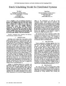
The design and development of distributed embedded systems driven by the TimeTriggered paradigm [33] has proven effective in a diversity of domains with stringent demands of determinism. Examples of time-triggered systems successfully deployed in the real world include the TTP-based [34] communication systems for the flight control computer of Embraer’s Legacy 450 and 500 jets and the distributed electric and environmental control of the Boeing 787 Dreamliner, whereas TTEthernet (SAE AS6802, [55]) has been selected for the NASA Orion Multi-Purpose Crew Vehicle [24], which successfully completed the Exploration Flight Test-1 (ETF-1) [41]. Ethernet-based time-triggered networks are key to enable the integration of mixed-criticality communicating systems in a scalable and cost-effective manner. Ongoing efforts within the IEEE 802.1 Time Sensitive Networking (TSN) task group [27] include the addition of time-triggered capabilities as part of Ethernet in the scope of the IEEE 802.1Qbv project [26]. TTEthernet is an extension to standard Ethernet currently used in mixed-criticality real-time applications. In TTEthernet a global communication scheme, the tt-network-schedule, defines transmission and reception time windows for each time-triggered frame being transmitted between nodes. The tt-network-schedule is typically built offline, accounting for the maximum end-to-end latency, message length, as well as constraints derived from resources and physical limitations, e.g., maximum frame buffer capacity. At runtime, a network-wide fault-tolerant time synchronization protocol [56] guarantees the cyclic execution of the schedule with sub-microsecond precision [31, p. 186]. The combination of these two elements allows for safety-critical traffic with guaranteed end-to-end latency and minimal jitter in co-existence with rate-constrained flows bounded to deterministic quality of service (QoS) and non-critical traffic (i.e. besteffort). In this paper we focus on TTEthernet as a key technology for safety-related networks and dependable real-time applications within the aerospace, automotive and industrial domains. The work we present throughout this paper, which is based on the work of Steiner [53], considers the typical case of multi-hop switched TTEthernet networks, such as the one depicted in Figure 1, in which the end-systems execute software tasks (i.e. tt-tasks1 ) following a similar time-triggered scheme (through static tabledriven CPU scheduling) communicating via the time-triggered message class of TTEthernet2 (i.e. tt-messages). The end-to-end latency is then subject to both scheduling domains: on the one hand the distributed network schedule, tt-networkschedule; and on the other hand the multiple dependent end-system schedules, tttask-schedules. The composition of the two scheduling domains is crucial to extend the end-to-end deterministic guarantees to include the application level, without disrupting the high determinism achieved at the network level. 1

The terms task and tt-task as well as message and tt-message will be used interchangeably in this paper. 2 Note that TTEthernet supports three traffic classes, namely time-triggered (TT), rateconstrained (RC), and best-effort (BE). We explicitly base this work on the TT traffic class in order to establish a time-triggered paradigm across the network and application domains. Extending the results presented in this paper to accommodate other traffic classes is a concern currently being addressed in the context of mixed-criticality systems (e.g.[54], [57])

2

Separate sequential schedule synthesis, either by scheduling the network first (e.g. [53]) and using the result as input for the task schedule synthesis [14], or the complementary approach [23], does not cover the whole solution space. Considering tasks and communication as part of the same scheduling problem enables an exhaustive search of the whole solution space guaranteeing that, if a feasible schedule exists, it will be found. We address this issue by considering the simultaneous co-synthesis of tt-network-schedules for TTEthernet as well as tt-task-schedules for the respective end-system CPUs. This approach broadens the scope of the timetriggered paradigm to include preemptable interdependent application tasks with arbitrary communication periods over multi-speed TTEthernet networks. We model the CPUs as self-links on the end-systems and schedule virtual frames representing non-preemptable chunks of preemptable tt-tasks. With this abstraction we formulate a general scheduling problem as a set of first-order logical constraints, the solving of which is known to be an NP-complete problem. We show that satisfying the end-to-end constraints and finding a solution for the whole problem set (using a one-shot approach) is possible for small system configurations, but does not scale well to large networks. Therefore, we present a novel incremental approach based on the utilization demand bound analysis for asynchronous tasks [7] using the earliest deadline first (EDF) algorithm [37], significantly improving the scalability factor with respect to the one-shot method. We introduce two alternative mechanisms for the resolution of the one-shot and incremental scheduling problems, based on Satisfiability Modulo Theories (SMT) and Mixed Integer Programming (MIP). In the first case, we transform the set of logical constraints into an SMT problem and allow the solver to synthesize a feasible schedule. We complement our evaluation using two state-of-the-art SMT solvers and provide a rough performance comparison in the orders of magnitude. For the second case, we introduce an optimization criteria as part of the scheduling constraints and formulate the problem as an MIP problem3 . The scalability of the two methods when solved with either SMT or MIP formulation suggests different performance trends, which we analyze with an open discussion summarizing the suitability of each approach. We specifically show that, even when using optimization, most of our problem sizes are solvable using the incremental demand method, which provides significant better scalability than prior existing methods. Thus, we claim to solve significantly harder problems of larger size, both when using SMT and when optimizing certain global problem objectives. This paper is an extended version of our previous work [13] which we broaden as follows. We have enhanced the network model to allow end-to-end latencies of periodic communication flows larger than the period. We also address in more detail the inherent problems introduced by limited resource availability, like memory, during the scheduling process. Moreover, we show how to transform the first-order logical constraints into a Mixed Integer Programming (MIP) problem, thus enabling optimization criteria to be specified as part of the scheduling formulation. This step enables us to extend the evaluation and scalability analysis providing performance figures for both approaches, which we complement using two alternative state-of3

We have identified a clear performance disparity between available MIP solvers, which in practice has limited our evaluation scope to a single one of the state-of-the-art MIP solver.

3

the-art SMT solvers and an additional MIP solver. Finally, we present an extended scalability discussion based on the evaluation results for both approaches (SMT and MIP) and show how the algorithm scales in each case. In Section 2, we define the system model that we later use to formulate logical constraints describing a combined network and task schedule in Section 3. In Section 4 we introduce two scheduling algorithms based on SMT, which we evaluate in Section 6 using industry-sized synthetic benchmarks. In Section 5 we show how to transform the logical constraint formulation into an optimization problem and discuss the feasibility using an MIP implementation of our method (Section 6). We review related research in Section 7 and conclude the paper in Section 8.

2

System Model

A TTEthernet network is in essence a multi-hop layer 2 switched network with full-duplex multi-speed Ethernet links (e.g. 100 Mbit/s, 1 Gbit/s, etc.). We formally model the network, similar to [53], as a directed graph G(V, L), where the set of vertices (V) comprises the communication nodes (switches and end-systems) and the edges (L ⊆ V × V) represent the directional communication links between nodes. Since we consider bi-directional physical links (i.e. full-duplex), we have that ∀[va , vb ] ∈ L ⇒ [vb , va ] ∈ L, where [va , vb ] is an ordered tuple representing a directed logical link between vertices va ∈ V and vb ∈ V. In addition to the network links, we also consider tasks running on the end-system nodes. We model the CPU of these nodes as directional self-links, which we call CPU links, connecting an end-system vertex with itself. A network or CPU link [va , vb ] between nodes va ∈ V and vb ∈ V is defined by the tuple h[va , vb ].s, [va , vb ].d, [va , vb ].mti, where [va , vb ].s is the speed coefficient, [va , vb ].d is the link delay, and [va , vb ].mt is the macrotick. In the case of a CPU link, the macrotick represents the hardwaredependent granularity of the time-line that the real-time operating system (RTOS) of the respective end-system recognizes. Typical macroticks for time-triggered RTOS ranges from a few hundreds of microseconds to several milliseconds [10, p. 266]. In the case of a network link the macrotick is the time-line granularity of the physical link, resulting from e.g. hardware properties or design constraints. Typically, the TTEthernet time granularity is around 60ns [32] but larger values are commonly used. The link delay refers to either the propagation and processing delay on the medium in case of a network link or the queuing and software overhead for a CPU link. The speed coefficient is used for calculating the transmission time of the frame on a particular physical link based on its size and the link speed. For a network link the speed coefficient represents the time it takes to transmit one byte. Considering the minimum and maximum frame sizes in the Ethernet protocol of 84 and 1542 bytes (including the IEEE 802.1Q tag), respectively, the frame transmission time, for example, on a 1Gbit/sec link would be 0.672µsec and 12.336µsec, respectively. For a CPU link, the speed coefficient is used to allow heterogeneous CPUs with different clock rates, resulting in different WCETs for the same task. 4

TT

EA

TT

TT

TT E-S wit ch

1

EB

E-S wit ch

TT

2

TT TT

EC

EE

ED

physical link communication path

Figure 1: A TTEthernet network with 5 end-systems and 2 switches. We denote the set of all tt-tasks in the system by Γ. A tt-task τiva ∈ Γ running on the end-system va is defined, similar to the periodic task model from [37], by the tuple hτiva .φ, τiva .C, τiva .D, τiva .T i, where τiva .φ is the offset, τiva .C is the WCET, τiva .D is the relative deadline, and τiva .T is the period of the task. Note that, a tt-task is pre-assigned to one end-system CPU and does not migrate during run-time4 . Hence, all task parameters are scaled according to the macrotick and speed of the respective CPU link. We denote the set of all tasks that run on end-system va by Γva . We model time-triggered communication via the concept of virtual link (VL), where a virtual link is a logical data-flow path in the network from one sender node to one receiver node. This concept is similar to [5] extended to include the tt-tasks associated with the generation and consumption of the message data running at the end-systems5 . We distinguish three types of tt-tasks, namely, producer, consumer, and free tt-tasks. Producer tasks generate messages that are being sent on the network, consumer tasks receive messages that arrive from the network, and free tasks have no dependency towards the network. Note that we assume that the actual instant of sending and receiving tt-messages occurs at the end and at the beginning of producer and consumer tasks, respectively. Considering the exact moment in the execution of a task where the communication occurs (cf. [17]) may improve schedulability, but remains out of the scope of this work. A typical virtual link vli ∈ VL from a producer task running on end-system va to a consumer task running on end-system vb , routed through the nodes (i.e. switches) v1 , v2 , . . . , vn−1 , vn is expressed, similar to [53], as vli = [[va , va ], [va , v1 ], [v1 , v2 ], . . . , [vn−1 , vn ], [vn , vb ], [vb , vb ]]. Note, however, that through this model it is also possible to exclude the tasks from the represented system in order to obtain network-only schedules. This is of particular interest for systems in which a synchronization between the CPU and 4

The assignment of tasks to CPUs is completely done during design time and corresponds to system requirements as well as other physical constraints (e.g. sensing tasks assigned to the node where the sensors are physically connected). 5 Note that in [5] virtual links are defined as multicast, e.g. with one sender and one or more receivers whereas in this work we constrain VLs to being unicast, e.g. one sender and one receiver. Our model can be extended to support multicast VLs without compromising the validity of the methods. For the sake of simplicity we leave this trivial extension as future work.

5

network domains is not established and the time-triggered paradigm is applied at the network level (e.g. [53]), or those in which the combined schedule is performed iteratively (e.g. [14]). Additionally vli .max latency denotes the maximum allowed end-to-end latency between the start and the end of the VL. Each task, regardless if it is a consumer, producer or free task, is associated with a virtual link. For communicating tasks, a virtual link is composed by the path through the network and the two end-system CPU links [va , va ] and [vb , vb ]. For a free task τiva ∈ Γ, a virtual link vli is created offline with vli = [[va , va ]]. Please note that, in TTEthernet, the VLs are statically specified and modelled and are not dynamically added in the system at runtime. Our goal is to schedule virtual links considering the task- and network-levels combined. Hence, we take both the tt-message that is sent over the network and the computation time of both producer and consumer tt-tasks and unify these through the concept of frames. Let M denote the set of all tt-message in the system. We model a tt-message mi ∈ M associated with the virtual link vli by the tuple hTi , Li i, where Ti is the period and Li is the size in bytes. For the network links, a frame is understood as the instance of a tt-message scheduled on a particular link. For CPU links, we model tasks as a set of sequential virtual frames that are transmitted (or dispatched) on the respective CPU link. Since we consider preemptive execution, we split the WCET of each task into virtual frames units based on the CPU macrotick and speed. Hence, we defined τiva .C to be the WCET of the task scaled according to the macrotick and speed of its CPU link. Therefore we have τiva .C non-preemptable chunks (i.e. virtual frames) of a task τiva . The split in non-preemptable chunks happens naturally through the macrotick of the underlying runtime system. In order to generalize frames scheduled on physical links and virtual frames scheduled on CPU links we say that a virtual link vli will generate sets of frames on every link (CPU or network) along the communication path. In the case of a network link the set will contain only one element, which is the (non-preemptable) frame instance of tt-message mi , whereas in the case of a CPU link the cardinality of the set will be given by the computation time of the task generating the virtual frames. Let F be the set of all frames in the system. We denote the ordered set of [v ,v ] all frames fi,ja b of virtual link vli scheduled on a (CPU or network) link [va , vb ] by [v ,v ] Fi a b ∈ F, the ordering being done by frame offset. Furthermore, we denote the [v ,v ] [v ,v ] [v ,v ] first and last frame of the set Fi a b with fi,1a b and last(Fi a b ), respectively. [v ,v ] [v ,v ] We use a similar notation to [53] to model frames. A frame fi,ja b ∈ Fi a b is defined by the tuple [v ,vb ]

hfi,ja

[v ,vb ]

.φ, fi,ja

[v ,vb ]

.π, fi,ja

[v ,vb ]

.T, fi,ja

.Li,

[v ,v ]

[v ,v ]

where fi,ja b .φ is the offset in macroticks of the frame on link [va , vb ], fi,ja b .π is [v ,v ] the initial period instance, fi,ja b .T is the period of the frame in macroticks, and [v ,v ] fi,ja b .L is the duration of the frame in macroticks. For a network link we have [v ,v ] fi,1a b .T

   Ti Li × [va , vb ].s [va ,vb ] , fi,1 .L = . = [va , vb ].mt [va , vb ].mt 

6

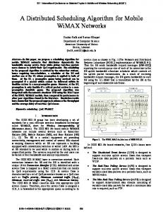
Note that in practical TTEthernet implementations, the scheduling entities are not frames but frame windows. A frame window can be larger than the actual transmission time of the frame, in order to account for the possible blocking time of low-priority (e.g. BE- or RC-) frames whose transmission was initiated instants before the TT-frame is scheduled. Since TTEthernet does not implement preemption of frames, methods like timely block or shuffling have been implemented in practice [62, p. 42-5]. With shuffling the scheduling window of TT-frames includes the maximum frame size of other frames that might interfere with the sending of TT-frames, while the timely block method will prevent any low-priority frame to be send if it would delay a scheduled TT-frame [62, p. 42-5], [55]. We consider the second mechanism although our findings can be applied to both algorithms. [v ,v ] A tt-task τivl ∈ Γ yields a set of frames fi,jl l , j = 1, 2, . . . , τivl .C, where each frame has size 1 (macrotick) and a period equal to the scaled task period, i.e., v τ l .T [v ,v ] fi,jl l .T = d [vl ,vi l ].mt e. The division in chunks comes naturally from the system macrotick, i.e., preemptive tasks can only be preempted with a granularity of 1 macrotick, allowing us to define sets of frames (chunks of task execution) for each task, essentially transforming the preemptive task model into a non-preemptive one with no loss of generality. Consequently, with this model, it is also possible to specify non-preemptive tasks by means of generating a single frame with length equal to its WCET. Our approach therefore implicitly supports non-preemptive task schedule synthesis (cf. [30], [61]) as it is a subproblem of preemptive task schedule synthesis. [v ,v ] The initial period instance (denoted by fi,ja b .π) is introduced to allow end-toend communication exceeding the period boundary. We model the absolute moment in time when a frame is scheduled by the combination of the offset –bounded within [v ,v ] [v ,v ] [v ,v ] the period interval– and the initial period instance, i.e., fi,ja b .φ+fi,ja b .π×fi,ja b .T . To better illustrate the concept of the initial period instance consider the two examples depicted in Figure 2. For communication with end-to-end latency (E2E) smaller than or equal to the period length, the initial period instance is 0 for all frames involved in the communication. In essence, the first and last frame instances of a message are transmitted within the same period instance. However, if the end-to-end latency is allowed to be greater than or equal to the period, the initial period instance can be larger than one. In the example depicted in Figure 2 with E2E ≥ T , the initial period instance for the frame on Linki+1 is 1, hence, the first frame instance of the VL on the link is scheduled at time 1 relative to its period but at time 6 relative to time 0.

3

Scheduling Constraints

Creating static time-triggered tt-schedules for networked systems, like the one described in this paper, generally reduces to solving a set of timing constraints. In this section we formulate, based on our system model, the mandatory constraints to correctly schedule, in the time-triggered sense, both tt-tasks and tt-messages. Some of our constraints (namely those in Sections 3.2, 3.3, 3.4, and 3.8) are similar to the contention-free, path-dependent, end-to-end transmission, and memory constraints from [53] but generalized according to our system definition to include virtual frames

7

Start period instance (Link i+1) = 0

Start period instance (Link i+1) = 1

Link i

0

5

10

15

0

5

10

15

0

5

10

15

5

10

15

Link i+1

0

E2E > T

E2E < T T (Period)

Figure 2: Communication over two links with different start period instances. generated by tasks, arbitrary macrotick granularity, and multiple link speeds.

3.1

Frame constraints

For any frame scheduled on either a network or CPU link, the offset cannot take any negative values or any value that would result in the scheduling window exceeding the frame period. Therefore, we have [v ,v ]

[v ,v ]

∀vli ∈ VL, ∀[va , vb ] ∈ vli , ∀fi,ja b ∈ Fi a b :     [v ,v ] [v ,v ] [v ,v ] [v ,v ] fi,ja b .φ ≥ 0 ∧ fi,ja b .φ ≤ fi,ja b .T − fi,ja b .L . The constraint bounds the offset of each frame to the period length, ensuring that the whole frame fits inside the said period. Note that if the end-to-end latency is allowed to be larger than the period, this constraint restricts CPU frames of a tt-task to remain within the same period instance, hence discarding placements in which the task execution starts in one period instance and extends to a following one. While this restriction reduces the search space and may potentially deem a valid configuration unfeasible, it simplifies by a significant amount the complexity involved in guaranteeing that no two tasks scheduled on the same CPU overlap. Relaxing this restriction would imply extending the non overlapping constraint to incorporate the subsequent period instances, which potentially leads to very complex formulations when the overlap can occur across the boundaries of the hyperperiod. If we consider end-to-end latencies less than or equal to the period, the initial period for each frame is always initialized at 0 (i.e. ∀f ∈ F : f.π = 0). Otherwise, we have to bound them such that the maximum end-to-end latency of the respective VL is not exceeded. We therefore have [v ,v ]

[v ,v ]

∀vli ∈ VL, ∀[va , vb ] ∈ vli , ∀fi,ja b ∈ Fi a b : ' ! &   vli .max latency [v ,v ] [v ,v ] −1 . fi,ja b .π ≥ 0 ∧ fi,ja b .π ≤ [v ,v ] fi,ja b .T

3.2

Link constraints

The most essential constraint that needs to be fulfilled for time-triggered networks is that no two frames that are transmitted on the same link are in contention, i.e., 8

they do not overlap in the time domain. Similarly, for CPU links, no tasks running on the same CPU may overlap in the time domain, i.e., no two chunks from any [v ,v ] [v ,v ] task may be scheduled at the same time. Given two frames, fi,ja b and fk,la b , that are scheduled on the same link [va , vb ] we need to specify constraints such that the frames cannot overlap in any period instance. [v ,v ]

[v ,v ]

[v ,v ]

[v ,v ]

[v ,v ]

[v ,vb ]

∀[va , vb ] ∈ L, ∀Fi a b , Fk a b ⊂ F, ∀fi,ja b ∈ Fi a b , ∀fk,la b ∈ Fk a # " # " k,l k,l HPi,j HPi,j ∀α ∈ 0, [va ,v ] − 1 , ∀β ∈ 0, [va ,v ] − 1 : fi,j b .T fk,l b .T   [v ,v ] [v ,v ] [v ,v ] [v ,v ] [v ,v ] fi,ja b .φ + α × fi,ja b .T ≥ fk,la b .φ + β × fk,la b .T + fk,la b .L ∨   [va ,vb ] [va ,vb ] [va ,vb ] [va ,vb ] [va ,vb ] fk,l .φ + β × fk,l .T ≥ fi,j .φ + α × fi,j .T + fi,j .L , def

[v ,v ]

,

[v ,v ]

k,l where HPi,j = lcm(fi,ja b .T, fk,la b .T ) is the hyperperiod of the two frames being compared. Please note that the contention-free constraints from [53] compare two frames over the cluster cycle (the hyperperiod of all frames in the system) whereas our approach only considers the hyperperiod of the two compared frames. The macrotick is typically set to the granularity of the physical medium. However, we can use this parameter to reduce the search space simulating what in [53] is called a scheduling “raster”. Hence, increasing the macrotick length –for a network or CPU link– reduces the search space for that link, making the algorithm faster, but also reduces the solution space. Additionally, a large macrotick for network links will waste bandwidth since the actual message size will be much smaller than the scaled one. A method employed by some applications, but not considered in our approach, is to aggregate similar VLs (similar in terms of sender/receiver nodes and period) into one message consuming one macrotick slot in order to reduce the amount of wasted bandwidth. Note, however, that the typical macrotick lengths of network and CPU links are several orders of magnitude apart, and that taking advantage of the scheduling raster for network links may be more beneficial than for CPU links. On one hand, the transmission of frames on a network link is non-preemptable and, therefore, using a scheduling raster smaller than the size of a frame transmission may increase significantly the required time to find a valid schedule with only a marginal increase on the number of feasible solutions. Moreover, for low utilized network links, which are not uncommon, larger rasters may still lead to valid solutions with a much reduced search space. The utilization on CPU links, on the other hand, is typically higher and requires tighter scheduling bounds, which are not possible with large rasters. Moreover, tasks are preemptable, and therefore, using a larger raster size than the operating system macrotick reduces the possible preemption points significantly decreasing the chances of success.

3.3

Virtual link constraints

We introduce virtual link constraints which describe the sequential nature of a communication from a producer task to a consumer task. The generic condition that 9

applies for network as well as for CPU links is that frames on sequential links in the communication path have to be scheduled sequentially on the time-line. Virtual frames of producer or consumer tasks are special cases of the above condition. All virtual frames of a producer task must be scheduled before the scheduled window on the first link in the communication path. Conversely, all virtual frames of the consumer task must be scheduled after the scheduled window on the last network link in the communication path. End-to-end communication with low latency and bounded jitter is only possible if all network nodes (which have independent clock sources) are synchronized with each-other in the time domain. TTEthernet provides a fault-tolerant clock synchronization method [56] encompassing the whole network which ensures clock synchronization. On a real network, the precision achieved by the synchronization protocol is subject to jitter in the microsecond domain. Hence, we also consider, similar to [61], the synchronization jitter which is a global constant and describes the maximum difference between the local clocks of any two nodes in the network. We denote the synchronization jitter (also called network precision) with δ, where typically δ ≈ 1µsec [31, p. 186]. ∀vli ∈ VL, ∀[va , vx ], [vx , vb ] ∈ vli : [v ,vb ]

[vx , vb ].mt × fi,1x

.φ − [va , vx ].d − δ ≥ [va ,vx ]

[va , vx ].mt × (last(Fi

[va ,vx ]

).φ + last(Fi

).L).

[v ,v ]

We remind the reader that last(Fi a x ) represents the last frame in the ordered set [v ,v ] Fi a x . The constraint expresses that, for a frame, the difference between the start of the transmission window on one link and the end of the transmission window on the precedent link has to be greater than the hop delay for that link plus the precision for the entire network. For end-to-end latencies larger than the period (i.e. non-zero initial period instance) we extend the previous condition as follows: ∀vli ∈ VL, ∀[va , vx ], [vx , vb ] ∈ vli : [v ,vb ]

([vx , vb ].mt × fi,1x

.φ − [va , vx ].d − δ ≥ [va ,vx ]

[va , vx ].mt × (last(Fi [v ,v ] (fi,1x b .π

>

[va ,vx ]

).φ + last(Fi

).L))∨

[v ,v ] last(Fi a x ).π).

As mentioned briefly in Section 2, the virtual link constraints are pessimistic for the CPU links in the sense that it is assumed that the sending and receiving of messages happens at the end and at the beginning of a producer and a consumer task, respectively. Schedulability may improve if the assumption is relaxed by considering the exact moment in the execution of a task where the message is sent or received. An example of such an approach can be found in [17] where schedulability in LETbased fixed-priority systems is improved at the expense of portability. This requires analysis and annotation of the project-specific source code and is outside the scope of this paper. However, the extension to allow such methods is trivial since it only 10

implies a change in constraints that would allow overlapping frames between task virtual frames and the transmission window of the associated communication frames.

3.4

End-to-End Latency constraints

Let src(vli ) and dest(vli ) denote the CPU links on which the producer task and, respectively, the consumer task of virtual link vli are scheduled on. We introduce latency constraints that describe the maximum latency of a communication from a producer task to a consumer task, namely ∀vli ∈ VL : dest(vli )

dest(vli ).mt × (last(Fi src(vli ).mt ×

src(vl ) fi,1 i .φ

dest(vli )

).φ + last(Fi

).L) ≤

+ vli .max latency.

In essence, the condition states that the difference between the end of the last chunk of the consumer task and the start of the first chunk of the producer task has to be smaller than or equal to the maximum end-to-end latency allowed. For the experiments in this paper we consider the maximum end-to-end latency to be smaller than or equal to the message period (which is the same as the period of the associated tasks). For non-zero start period instances we extend the previous constraint as follows: ∀vli ∈ VL : dest(vli )

dest(vli ).mt × (last(Fi src(vli )

src(vli ).mt × (fi,1

3.5

dest(vli )

).φ × last(Fi

src(vli )

.φ × fi,1

dest(vli )

).π + last(Fi

).L) ≤

.π) + vli .max latency.

Task constraints

For any sequence of virtual frames scheduled on a CPU link, the first virtual frame has to start after the offset defined for the task and the last virtual frame has to be scheduled before the deadline specified for the task. In order to finish the computation before the deadline, the offset has to be at most the deadline minus the computation time. Hence, we have     [v ,v ] [v ,v ] ∀va ∈ V, ∀τiva ∈ Γva : fi,1a a .φ ≥ τiva .φ ∧ last(Fi a a ).φ ≤ τiva .D − τiva .C .

3.6

Virtual frame sequence constraints

For a CPU link, we check in the condition in Section 3.2 that the scheduling windows of virtual frames generated by different tasks do not overlap. Additionally, we have to check that virtual frames generated by the same task do not overlap in the time domain. This condition can be expressed similar to the condition in Section 3.2, however, we express it, without losing generality, in terms of the ordering of the virtual frame set. h  i [va ,va ] [v ,v ] [v ,v ] [va ,va ] va va .φ ≥ fi,ja a .φ + fi,ja a .L. ∀va ∈ V, ∀τi ∈ Γ , ∀j ∈ 1, Fi − 1 : fi,j+1 11

3.7

Task precedence constraints

Task dependencies are usually expressed as precedence constraints [11], e.g., if task τiva and τjvb have precedence constraints (τiva ≺ τjvb ) then τiva has to finish executing before τjvb starts. Even though these dependencies arise typically between tasks co-existing on the same CPU, we generalize dependencies between tasks executing on any end-system. Task dependencies are partially expressed in [53] as frame dependencies in the sense that one frame is scheduled before another frame, which can be used to specify aspects of the existing task schedule. We introduce constraints for simple task precedences in our model as follows [v ,vb ]

τiva ≺ τjvb ⇒ [vb , vb ].mt × fj,1b [va , va ].mt ×

[v ,v ] (last(Fi a a ).φ

.φ ≥ [va ,va ]

+ last(Fi

).L).

Note that, in our model, both tasks have the same period or “rate”. Including multi-rate precedence constraints (extended precedences as they are called in [19]) for periodic tasks is a restriction of our implementation and model rather than a restriction of our method. Extending the model to handle extended precedences for periodic tasks, even if the periods differ from one another, implies that tasks are not represented by a sequence of frames that repeats with the period but by multiple instances of the frames that repeat with the hyperperiod of the two dependent tasks. The dependency is then expressed as constraints between individual frames from the multiple instances of the tasks where the pattern of dependency is selected by the system designer. We elaborate on one example. If a “slow” task τi with period Ti = n · Tj must consume the output of a “fast” task τj with period Tj , the system designer may choose, for example, that n outputs of τj are selected as inputs for one instance of τi or that only the last output of τj is considered as input for τi . In both cases, the implementation of task τi is responsible for representing this dependency. In terms of logical constraints, these are easily added since they imply adding logical constraints between frames, i.e., each nth frame of task τj has to be scheduled before the corresponding frame of τi . Note, however, that this only applies to periodic tasks since aperiodic tasks cannot be represented by a finite set of frame instances.

3.8

Memory constraints

Resource constraints come into play when the generated schedule is deployed on a particular hardware component. One such constraint is derived from the availability of physical memory necessary to buffer frames at each network switch. Taking as an example a message forwarded through a switch, the incoming frame needs to be buffered from the moment when it arrives in the ingress port (i.e. scheduled arrival time6 ) until the following frame is transmitted via the egress port (i.e. end of the scheduled transmission window). During runtime, at any instant each device shall satisfy that the memory demand for all buffered frames fits within their available physical memory. 6 Note that despite we do not implicitly synthesize a schedule for the incoming frames the arrival schedule is a trivial transformation of the related schedules of the predecessor frames.

12

fin fout H Network cycle

Figure 3: Simplified example of a memory demand histogram. 3.8.1

Offline buffer demand calculation

As a property of the time-triggered paradigm, the arrival and departure times of tt-frames are known from the schedule. Therefore, a buffer demand histogram, similar to [51], for each network device can be constructed offline. The range of the histogram shall cover the entire network cycle and the interval size be equal to the raster size. Let H(hp) be an array, where hp is the network cycle length defining the number of bins, the following post-analysis performed on a given switch x upon generation of a valid schedule populates the histogram Hx with the buffer demand at each macrotick along the network cycle (i.e. histogram bin): ∀x ∈ V, ∀vli ∈ VL, ∀k, 0 ≤ k ≤ hp : X [v ,v ] [v ,v ] [v ,v ] hit(fi,1a x .φ, last(Fi x b ).φ + last(Fi x b ).L, k) Hx (k) = ∀[va ,vx ],[vx ,vb ]∈vli

where ( 1 if tin ≤ k ≤ tout hit(tin , tout , k) = 0 else Figure 3 depicts the memory demand histogram for a simplified example. Note that fin represents the set of scheduled windows for incoming frames in the analyzed device with independence of their VL and incoming port, respectively, fout shows the scheduled windows for the outgoing frames. Arrows indicate the sequence relation between incoming and outgoing frames. The memory histogram, below, increases for each scheduled incoming frames and decreases for each outgoing frame. Note that the model of the memory management system assumes the ability of allocating and releasing memory buffers at, respectively, the beginning and end of every macrotick. We also assume the size of buffers constant and fixed (e.g. maximum frame size). Note, however, that since the analysis is done offline accounting for variable buffer sizes as well as discrete instants of time (e.g. at the beginning or end of a period) are trivial extensions. Once the histogram is built, the following condition must hold to guarantee that

13

the buffer demand will be satisfied at runtime, ∀vx ∈ V, ∀k, 0 ≤ k ≤ hp : Hvx (k) ≤ vx .ω, where vx .ω is the maximum number of buffers that the device vx can simultaneously allocate. 3.8.2

Online time-based buffer demand constraint

Unfortunately, including the above condition as part of the SMT constraint formulation and force the scheduling process to maintain the buffer demand below a given bound is non-trivial. The derived constraints require the use of quantifiers, which degrade significantly the solver performance and are not widely supported by all SMT engines. To circumvent this limitations, we introduce an alternative online memory constraint, similar to [53], based on the same principle used for the construction of the buffer demand histogram. In essence, we introduce vx .b, a parameter defining an upper bound on the time that node vx ∈ V is allowed to buffer any given ingress frame before scheduling the corresponding egress frame. Limiting the time a frame can be buffered essentially reduces the maximum number of frames that may simultaneously coexist within the device memory, hence lowering the buffer demand bound. The time-based memory constraint for any given device remains as follows: ∀vli ∈ VL, ∀[va , vx ], [vx , vb ] ∈ vli : [v ,vb ]

[vx , vb ].mt × fi,1x

[v ,vx ]

.φ − [va , vx ].mt × fi,1a

.φ ≤ vx .b

While this condition does not directly reflect the maximum buffer demand it allows a straight forward formulation as SMT constraint. An offline analysis based on the memory demand histogram as described in 3.8.1 allows to adjust b for those nodes exceeding the resource capacity in an iterative process. However, it is also possible to pre-calculate a pessimistic upper bound for the memory demand based on the worst case scenario. Starting from an initial state without any buffer being allocated at instant t0 and assuming the set Lvx ⊂ L, and ∀va ∈ V, vx ∈ V ⇒ [va , vx ] ∈ Lvx . We define a maximum flow schedule in which for every link [va , vx ] ∈ Lvx a frame f [va ,vx ] is scheduled at every following macrotick [va , vx ].mt with f [va ,vx ] .L = 1 and buffered for the maximum allowed time. In essence, this is equivalent of assuming that for each ingress port of a device (i.e. physical link towards the device7 ), there will be a continuous burst of incoming frames, which remain buffered for the maximum allowed time. Note that the relation of frames and virtual links is irrelevant since we only care about the flow of incoming frames. Figure 4 illustrate an example of a device vx ∈ V with 4 ingress ports and the respective maximum flows characterized by the respective frames f [vα ,vx ] ,f [vβ ,vx ] , f [vγ ,vx ] , f [vδ ,vx ] . Since the time-based memory constraint ensures that frames remain buffered at most b units of time, at time t0 +b the accumulated buffer demand will be maximum. 7

Note that physical links and by extension also ports are full-duplex, and therefore, each ingress port has an egress port as counterpart. For this analysis we only need to consider incoming traffic.

14

f

[vα ,vx]

f

[vβ ,vx]

f

[vδ ,vx]

Vx

f

[vγ ,vx]

Figure 4: Example of a device (vx ) with four ingress ports. From that moment on, for every additional incoming frame there will be one frame leaving the device. In essence, the memory bound m ˜ for device vx results from   X vx .b m(v ˜ x) = [va , vx ].mt ∀[va ,vx ]∈Lvx

Note, however, the pessimism in this estimation as not only it assumes the maximum concurrent communication flow (e.g. full link utilization), but also the frame length equal to one macrotick. In practice, the utilization of physical links will remain at a lower capacity and frame length may exceed the macrotick length, hence lowering the total number of incoming frames during the burst interval.

3.9

Schedule and constraints example

We present a simplified example of a schedule in Figure 5 to better illustrate our model and the various constraints described above. We consider a simple network with two end-systems va and vb (and the CPU links on the end-systems [va , va ] and [vb , vb ]) connected through a network link ([va , vb ]). For the CPUs and the link we assume that all are defined by the tuple h1, 1, 1i, i.e., speed, delay and macrotick are 1. There are 4 tasks (2 consumers and 2 producers) in the system. τ1 and τ3 run in va (scheduled on the CPU link [va , va ]), and τ2 and τ4 run in vb (scheduled on the CPU link [vb , vb ]). τ1 with computation time 3 macroticks communicates to τ2 with 2 macroticks computation time through message m1 (vl1 ). τ3 with 2 macroticks computation time communicates to τ4 which has a WCET of 2 macroticks through message m2 (vl2 ). All tasks and the associated messages have period 20 macroticks. Both messages have a message length which translates to 1 macrotick on the link. Additionally, there is a precedence constraint specifying that τ4 has to run before τ2 . The tasks generate virtual frames (chunks) on the respective links proportional [v ,v ] [v ,v ] [v ,v ] to their computation time, e.g. τ1 generates 3 virtual frames f1,1a a , f1,2a a , f1,3a a [v ,v ] [v ,v ] (pictured). Messages m1 and m2 generate one frame each, i.e., f1,1a b and f2,1a b , respectively.

15

[va,va]

f1[,1va ,va ]

f1[,2va ,va ]

f1[,3va ,va ]

0

5

10

f2[,v1a ,vb ]

[va,vb]

15

20

f1[,1va ,vb ]

0

5

10

15

20

0

5

10

15

20

[vb,vb]

Virtual link constraints

Precedence constraint

End-to-end latency constraint

τ1(0,3,7,20)

m1

τ2(3,2,20,20)

vl1

τ3(1,2,6,20)

m2

τ4(2,2,14,20)

vl2

Figure 5: Example of a schedule with 2 CPUs, 1 link, 2 VLs, and 4 tasks. The end-to-end latency constraint specifies that the time between the start of the producer task (e.g. τ1 ) and the end of the consumer task (e.g. tau2 ) of a VL has to be smaller than or equal to a certain value. In our example, the end-to-end latency constraint of vl2 is 12 macroticks. Hence, the schedule of the first frame (chunk) of τ3 and the last frame (chunk) of task τ4 are scheduled at most 12 macroticks apart. The virtual link constraint ensures that the gap between the last frame of τ3 and the frame of the message m2 on the link are at least δ (network precision) apart and in the correct order. The CPU and network delays (set to 1 in the example) result in the scheduled frames of the same virtual link on sequential (CPU or network) links [v ,v ] [v ,v ] (e.g. f1,3a a and f1,1a b ) to be at least 1 macrotick apart.

4

SMT-based co-synthesis

Satisfiability Modulo Theories (SMT) checks the satisfiability of logic formulas in first-order formulation with regard to certain background theories like linear integer arithmetic (LA(Z)) or bit-vectors (BV) [6], [50]. A first-order formula uses variables as well as quantifiers, functional and predicate symbols, and logical operators [40]. Scheduling problems are easily expressed in terms of constraint-satisfaction in linear arithmetic and are thus suitable application domains for SMT solvers; a good use-case presentation of using SMT for job-shop-scheduling can be found in [16]. Naturally, time-triggered scheduling fits well in the SMT problem space since infinite sequences of frames (and task jobs) can be represented through finite sets 16

Algorithm 1: One-shot SMT schedule synthesis Data: G(V, L), VL, M, Γ Result: S (tt-schedule) begin S ← ∅; if Check(V, Γ) ∧ Check(VL, M) then C ← Assert(G(V, L), VL, M, Γ); S ← SMTSolve (C); return S;

that repeat infinitely with a given period. However, event-based and non-periodic systems (which are out of scope of this paper) cannot be scheduled through SMT directly since their arrival patterns cannot be represented through a finite set. At its core, our scheduling algorithm generates assertions (boolean formulas) for the logical context of an SMT solver based on the constraints defined in Section 3 where the offsets of frames are the variables of the formula. For a satisfiable context, the SMT solver returns a so-called model which is a solution (i.e. a set of variable values for which all assertions hold) to the defined problem.

4.1

One-shot scheduling

The one-shot method (Algorithm 1) considers the whole problem set including all tt-tasks on all end-systems as well as all tt-messages. The inputs of the algorithm are the network topology G(V, L), the set of virtual links VL, the set of tt-messages M, and the set of tt-tasks Γ. The output is the set S of frame offsets or the empty set if no solution exists. First, the utilization on each end-system is verified (through the Check function) to be lower than 100% using the simple polynomial utilization-based test (cf. [37]) ∀va ∈ V :

X τ va .C i τiva ∈Γva

τiva .T

≤ 1.

This test is necessary but not sufficient, i.e., if the test fails, the system is definitely not schedulable since the demand of the task set exceeds the CPU bandwidth on at least one end-system, however, if the test passes, the system may or may not be schedulable. A similar check is employed for all network links and the corresponding frames since, in general, the density of feasible systems is less than or equal to 1 [36]. If the check is successful, the algorithm adds the constraints defined in Section 3 to the solver context C (Assert) and invokes the SMT solver (SMTSolve) with the constructed context as described above. The solution S (the solver model), if it exists, contains the values for the offset variables of all frames and is used to build the tt-schedule. The producer, consumer, and free tt-tasks as well as the tt-messages may generate, depending on the system configuration, a very large number of frames that need to be scheduled. It is known that such scheduling problems (which reduce to the 17

bin-packing problem) are NP-complete [53]. Hence, the scalability of the one-shot approach may not be suitable for applications with hundreds of tt-messages and large network topologies. In order to improve the performance and scalability of network-only schedule synthesis, Steiner [53] proposes an incremental backtracking approach which takes only a subset of the frames at a time and adds them to the SMT context. If a partial solution is found, additional frames and constraints are added until either the complete tt-network-schedule is found or a partial problem is unfeasible. In the case of un-feasibility, the problem is backtracked and the size of the increment is increased. In the worst case the algorithm backtracks to the root, scheduling the complete set of frames in one step. The performance improvement due to the incremental backtracking method may be sufficient when only scheduling network messages. However, when co-scheduling messages and tasks in large systems, the number of virtual frames due to tasks running on end-systems renders the problem impracticable. Moreover, our experiments with an incremental version of our one-shot algorithm have shown that it performs best when the utilization is low (which is often true for network links) since there is enough space on the links to incrementally add new frames without having to move the already scheduled ones. However, on CPU links, the utilization due to tasks is usually high, resulting in the incremental backtracking method performing worse than in the average case. Hence, the incremental backtracking approach proposed by Steiner is not suitable for our purpose. We present in the next section a novel incremental algorithm specifically tailored for task scheduling that reduces the runtime of combined task/network scheduling for the average case by taking into account the different types of tasks executing on end-systems.

4.2

Demand-based scheduling

Free tasks account for a significant amount of the total frames that need to be scheduled. However, these tasks do not present any dependency towards the network nor other end-system tasks. Hence, they do not need to be considered from the network perspective, but only from the end-system perspective. The main idea behind the demand-based method (Algorithm 2) is to schedule only communicating tasks via the SMT solver and check, afterward, if the resulting schedule on all end-systems is feasible when adding the corresponding free tasks. In [14] we have introduced a method to generate optimal static schedules using dynamic priority scheduling algorithms. We considered tasks as being asynchronous with deadlines less than or equal to periods (i.e., constrained-deadline task systems) and generated static schedule by simulating the EDF algorithm until the hyperperiod. We employ a similar method here for scheduling free tasks. In this way, free tasks do not add to the complexity of the SMT context but are scheduled separately, resulting in improved performance for the average case. This improvement does not come at the expense of schedulability. We guarantee this by doing an incremental approach that in a first step schedules communicating tasks and checks if, for any end-system, the resulting schedule after adding the free tasks would be schedula-

18

Algorithm 2: Demand-based SMT schedule synthesis Data: G(V, L), VL, M, Γ Result: S (tt-schedule) begin S ← ∅; if Check(V, Γ) ∧ Check(VL, M) then f ← f alse; Γedf ← Γf ree ; Γsmt ← Γ \ Γf ree ; while f 6= true do C ← Assert(G(V, L), VL, M, Γsmt ); S ← SMTSolve (C); if S = 6 ∅ then Γd ← DemandCheck(V, S, Γedf ); if Γd 6= ∅ then Γedf ← Γedf \ Γd ; Γsmt ← Γsmt ∪ Γd ; else f ← true; if Γedf 6= ∅ then S ← S ∪ EDFSim(V, S, Γedf ); else f ← true; return S;

ble. If this is the case, the free tasks are scheduled by simulating EDF until the hyperperiod. If the resulting system is not schedulable the algorithm increases the SMT formulation by adding only those free tasks that make the solution unfeasible and runs the solver over the increased set. This is done incrementally until either a solution is found or the whole set of free tasks has been added to the SMT problem without finding a solution. The inputs of the algorithm are, as before, the network topology G(V, L), the set of virtual links VL, the set of messages M, and the set of tasks Γ (cf. Algorithm 2). Like in the one-shot method, the utilization on all end-systems and all network links is verified (Check function) first. We define the following helper sets. The set of free tasks Γf ree is the set containing all tasks that are neither producer nor consumer tasks and which are not dependent on other tasks. We also introduce the set of tasks scheduled with SMT (Γsmt ) and the set of tasks scheduled with EDF (Γedf ). Initially, Γedf is equal to the set of free tasks Γf ree and Γsmt = Γ \ Γf ree is the set of remaining tasks from Γ. We repeat the following steps until either a solution is found or the set Γedf is empty. First, we add the constraints defined in Section 3 based on the tasks in Γsmt to the solver context C (Assert) and then invoke the 19

SMT solver (SMTSolve) with the constructed context. If no solution exists we exit from the loop and return the empty set. If there exists a partial solution S = 6 ∅, we check (via the function DemandCheck) the demand of the resulting system together with the tasks which have not yet been scheduled (the tasks in Γedf ). The demand check is based on the necessary and sufficient feasibility condition for constrained-deadline asynchronous tasks with periodic execution under EDF (cf. [7]). The test constructs a set of intervals between any release and any deadline over a certain time-window. In each of these intervals the demand of the executing tasks is checked to be smaller than or equal to the supply (the length of the interval). In our case, for every end-system, the set of tasks is derived from the already scheduled tasks in Γsmt and the tasks in Γedf . The already scheduled tasks in Γsmt have fixed scheduled intervals according to their virtual frames whereas the tasks in Γedf will be treated as EDF tasks. e va For every end-system va ∈ V the function DemandCheck generates a set Γ of virtual periodic tasks, where every virtual task τek va is defined by the tuple hτek va .φ, τek va .C, τek va .D, τek va .T i, consisting, as before, of the offset, the WCET, the relative deadline, and the period of the virtual task, respectively. For every task τiva ∈ Γedf we generate a virtual task τek va with a one to one translation of the task [v ,v ] parameters. Additionally, for every frame offset8 fi,ja a .φ ∈ S we generate a virtual [v ,v ] [v ,v ] task τek va with τek va .φ = fi,ja a .φ, τek va .C = 1, τek va .D = 1, and τek va .T = fi,ja a .T . We use the necessary and sufficient feasibility condition from [7], [45] for every eva , namely generated virtual task set Γ ∀va ∈ V, ∀t1 ∈ Φva , ∀t2 ∈ ∆va , t1 < t2 :      X t2 − τei va .φ − τei va .D t1 − τei va .φ va τei .C × − + 1 ≤ t2 − t1 , τei va .T τei va .T 0

e va τei va ∈Γ

where def eva , j ≥ 0, ava ≤ λva }, τi va ∈ Γ Φva = {avi,ja = τei va .φ + j × τei va .T |e i,j def

eva , j ≥ 0, dva ≤ λva }, τi va ∈ Γ ∆va = {dvi,ja = avi,ja + τei va .D|e i,j eva }). eva }) + 2 × lcm({e τ i va ∈ Γ τi va .T |e τi va ∈ Γ λva = max({e τi va .φ|e The sets Φva and ∆va of arrivals and absolute deadlines, respectively, define intervals in which the demanded execution time of running tasks has to be less than or equal to the processor capacity [7], [45]. If the test is fulfilled on every end-system, we know that applying EDF to the task sets will result in a feasible schedule. In this case, the function DemandCheck returns an empty set. We schedule the remainder of the tasks by running an EDF simulation (EDFSim) on each end-system of the entire virtual task set (composed of both scheduled and unscheduled tasks) until the hyperperiod. The EDF simulation will return the static schedule for the tasks in Γedf which will complete the partial solution S. If the schedulability condition is not fulfilled on some end-system, the function DemandCheck returns the set (Γd ) 8

Frames of the same task scheduled sequentially on the time-line can be joined into a bigger virtual task to increase the performance of the feasibility test.

20

of tasks that have contributed to the intervals where the demand was greater than the supply. These tasks are removed from the set Γedf and added to the set Γsmt and the procedure is repeated. The loop terminates (f ← true) when either a full solution is found or the SMT solver could not synthesize a partial schedule for Γsmt . In our current implementation, the decision of which tasks to move from Γedf to Γsmt in the case that the schedulability test is not fulfilled is taken based on the intervals in which the demand exceeds the available CPU bandwidth. More precisely, we select all tasks that run in the overloaded intervals. This decision criteria is an intuitive but not an optimal one since it may be that other tasks, which are not scheduled in the overloaded intervals, are actually causing the overload. However, an optimal criteria cannot be determined due to the domino effect (cf. [10, p. 37] or [52, p. 87]) in overload conditions. Nevertheless, since the DemandCheck function can be replaced with another method, heuristics can be employed to find decision criteria which better suit particular scheduling scenarios. Note that in the worst case, the algorithm may perform worse than the one-shot method due to the intermediary steps in which partial solutions were unfeasible. If none of the partial solutions were feasible, in the last step, the demand-based algorithm has to solve the same input set as the one-shot method. The feasibility test9 is known to be co-NP-hard [35, p. 615]. Therefore, the underlying scheduling problem still remains exponential in the worst case. However, the run-time of the test is highly dependent on the properties of the tasks (periods, harmonicity of periods, hyperperiod, etc.) which, in practice, are not that pessimistic. Moreover, with the one-shot method, all free tasks were considered in the same problem space even if they are running on separate end-systems and are thus independent of each-other. With the demand-bound method, we can evaluate the demand bound function for the free tasks on each end-system separately thus reducing the size of the problem even further. Hence, in the average case, the demand method may be more practicable than solving the entire problem using SMT, since splitting the problem and solving it using an incremental approach reduces the runtime for the average case in which only a few incremental steps are needed. Naturally, we do not improve the scalability of the underlying SMT solver, rather, we reduce, regardless of the algorithm complexity and without sacrificing schedulability, the size of the SMT problem and hence the number of assertions and frames that place a burden on the solver. Through this we can tackle medium to large problems even in the extended scenario of co-scheduling preemptive tasks together with messages in a multi-hop switched network. Moreover, finding a schedule with the SMT solver becomes harder the more utilized the links become. By eliminating subsets of tasks from the input of the SMT solver we make it easier for the SMT solver to place the (virtual) frames of the remaining tasks, thus shifting the complexity from the SMT solver to the schedulability test. We show in the experiments section that the demand method outperforms the one-shot and results in significant performance improvements leading to better scalability for medium to large input configurations. 9 Note that other tests with pseudo-polynomial complexity [44], [7] could be used instead, but these are only sufficient or deal with restricted task sets.

21

5

Optimized co-synthesis

The algorithms presented in the previous section, which are based on SMT, will retrieve a solution, if one exists, for the given scheduling problem. However, the solution is an “arbitrary” one10 out of a set of (potentially) multiple valid solutions. Each of these valid solutions might have a different impact with regard to several key schedulability and system properties. Examples of such key properties are endto-end latencies (which influence system performance and correctness) and memory consumption in switches (which enables efficient design of switch-hardware). For some systems the user might want to optimize one or several of these key properties. Generally, problems that have constraints on variables, like our scheduling problem, but also optimize some property of the system are known as constrained optimization problems. The basic constraint formulation as well as the scheduling model are not specific to SMT solvers but can be re-formulated to be compatible with different problem types. We can transform the task- and network-level schedule co-synthesis into a Mixed Integer Programming (MIP) problem with different objectives to minimize, such as end-to-end latency or memory buffer utilization. Virtual link, latency, precedence and frame constraints can be readily transformed into a MIP formulation since they do not contain any logical clauses. Logical either-or constraints, like the ones used in the link constraints (Section 3.2), express that at least one of the constraints must hold but not both. To transform this condition to a single inequality in MIP formulation we use the alternative constraints method (cf. [9, p. 278] or [8, p. 79]). The same method is used in [61]. Consider, [v ,v ] [v ,v ] as before, two frames, fi,ja b and fk,la b , that are scheduled on the same link [va , vb ] and cannot overlap in any period instance. For every contention-free assertion, as introduced in Section 3.2, we introduce a binary variable z ∈ {0, 1}, and formulate the either-or constraint as follows [v ,v ]

[v ,v ]

[v ,v ]

[v ,v ]

[v ,v ]

[v ,v ]

∀[va , vb ] ∈ L, ∀Fi a b , Fk a b ⊂ F, ∀fi,ja b ∈ Fi a b , ∀fk,la b ∈ Fk a b , # " # " k,l k,l HPi,j HPi,j ∀α ∈ 0, [va ,v ] − 1 , ∀β ∈ 0, [va ,v ] − 1 : fi,j b .T fk,l b .T   [v ,v ] [v ,v ] [v ,v ] [v ,v ] [v ,v ] fk,la b .φ − fi,ja b .φ − z × Ω ≤ α × fi,ja b .T − β × fk,la b .T − fk,la b .L ∧   [v ,v ] [v ,v ] [v ,v ] [v ,v ] [v ,v ] fi,ja b .φ − fk,la b .φ + z × Ω ≤ β × fk,la b .T − α × fi,ja b .T − fi,ja b .L + Ω , def

[v ,v ]

[v ,v ]

k,l where HPi,j = lcm(fi,ja b .T, fk,la b .T ), is, as before, the hyperperiod of the two frames and Ω is a constant that is large enough (in our case we choose the hyperk,l period HPi,j ) such that the first condition is always true for z = 1 and the second condition is always true for z = 0. The downside of this approach is that a lot of binary variables are introduced into the problem since link constraints represent a significant subset of all needed constraints. 10 By “arbitrary” we mean that the SMT solver will return the first valid solution that it finds which, depending on the implementation, is not chosen according to schedulability criteria but rather depends on the specific generic search mechanism of the solver.

22

Most industrial applications require the end-to-end latency of communication to be minimized (e.g. [20, p. 143], [42, p. 411], [43]). A minimal end-to-end latency may also reduce buffer utilization in switches since the duration of how long messages are stored for forwarding in switch buffers is minimized (cf. Section 3.8). We implemented this transformation on top of our previously presented algorithms and set as an objective to minimize the accrued end-to-end (E2E) communication latency, i.e., the sum of the E2E latencies of all virtual links in the network. We denote Λi to be the end-to-end communication latency of virtual link vli ,   dest(vli ) dest(vli ) src(vl ) Λi = dest(vli ).mt × last(Fi ).φ + last(Fi ).L − src(vli ).mt × fi,1 i .φ. Hence, the optimization problem can be specified as minimize,

X

vli ∈VL

Λi , subject to the constraints presented in Section 3.

vli ∈VL

We are not interested in minimizing any property of the free tasks, hence they are not present in the aforementioned objective. However, there may be properties of free tasks that are of interest for an optimization objective, like number of context switches which would reduce cache misses and system overhead, but these are beyond the scope of this paper. Since the transformation is built on top of the existing algorithms, both one-shot and demand-based algorithms can be employed with the difference that the SMTengine is replaced by an optimization engine. However, if the optimization objective includes properties of free tasks, the demand-based approach might not be suitable anymore or might require a more complex feedback loop to be implemented. In such cases a sequential schedule synthesis providing a solution with local optimization for the free tasks (cf. [14]) may be more practicable.

6

Evaluation

We implemented a prototype tool, called TT-NTSS, for task- and network-level static schedule co-generation based on the system model, constraint formulation, and scheduling algorithms described above. We introduced a generic solver interface enabling the abstraction of logical constraint formulation from the underlying SMT (or optimization) solver engine. In this way, we are able to reproduce the experiment with alternative SMT solvers and with different optimization engines without modifying core functionalities.

6.1

Configuration Set-Up

For the experimental evaluation with SMT solvers (see Section 6.2) in this paper, we have selected Yices v2.3.1 (64bit) [12] and Z3 v4.4.0 (64bit) [15] using linear integer arithmetic (LA(Z)) without quantifiers as the background theory. We show the results using both solver libraries running on a 64bit 8-core 3.40GHz Intel Core-i7 PC with 16GB memory. Note, however, that using alternate back-end solvers is not 23

Figure 6: Example network topologies: (a) Ring–size 6, (b) Mesh–size 6, (c) Tree– depth 2. All examples with 3 end systems per switch (leaf nodes only). Name P1 P2 P3

Periods (ms) {10, 20, 25, 50, 100} {10, 30, 100} {50, 75}

Hyperperiod (ms) 100 300 150

Table 1: Sets of periods and their respective hyperperiod. intended as a performance comparison between the solvers but rather a reinforcement of the feasibility claims to use SMT for scheduling problems. We aim, in this way, at confirming a similar trend with independence of the selected library and avoid, to some extent, unnoticed effects due to bugs or limitations inherent to one particular solver. The optimization results (see Section 6.3) were obtained using the 64bit version of the Gurobi11 Optimizer [22] v6.0 running on the same platform. For the sake of completeness, we intended to use the open-source GNU Linear Programming Kit [21] (GLPK) package on its version 4.54. However, during our evaluation we found out that the performance of GLPK is several orders of magnitude below that of Gurobi12 and the SMT approach, hence rendering the comparison uninteresting. Therefore, we reduce the comparison of the two to a minimum, and center our evaluation between the remaining three engines. We analyze the performance of TT-NTSS over a number of industrial-sized synthetic scenarios following the network topologies depicted in Figure 6. For each case we evaluate four network sizes which range from small (i.e. a couple of switches) to huge (i.e. several tens of switches). We scale proportionally the number of connected end systems and therefore the number of tasks to be scheduled. Table 2 summarizes the configuration for each scenario. For the experiments we use 3 different sets of communication periods, as listed in Table 1. Each end-system runs a total of 16 tasks without precedence constraints, of which 8 are communicating and 8 free. We choose this ratio as a representative proportion of free and communicating tasks based on our experience. Note, however, that the performance of the methods evaluated in this section is subject to the ratio between the accumulated utilization of free and communicating tasks, rather than the particular number of tasks. Therefore, the WCET of tasks is set 11

We thank Gurobi Optimization, Inc for their generous licensing support. This finding is reaffirmed in [38], in which the authors present a detailed performance comparison of several commercial and open-source MIP solvers for a particular problem domain. 12

24

Size Small (S) Medium (M) Large (L) Huge (H)

Topology Mesh, Ring Tree, depth = 1 Mesh, Ring Tree, depth = 2 Mesh, Ring Tree, depth = 3 Mesh, Ring Tree, depth = 2

Num Switches 2 4 4 13 8 15 16 43

Num End-Systems 4 6 16 36 48 48 192 432

Table 2: Configuration parameters for network configurations of each size. proportionally to the period and the desired CPU utilization bound, rounded to the nearest macrotick multiple. It is a common pattern in industrial applications that communicating tasks (e.g. sensing and actuating) are sensibly smaller than non-communicating ones (e.g. background computation and core functionality). Therefore, we choose to model free tasks to account for approximately 75% of the utilization and communicating tasks for 25%13 . We define virtual links between pairs of communicating tasks executing on distinct randomly-selected end systems. Among the communicating tasks, the producer or consumer role is decided randomly upon generation of the end-to-end communication. Message sizes are chosen randomly between the maximum and minimum Ethernet packet sizes, while the periods of tasks as well as their respective VLs are randomly distributed among the selected predefined set (see Table 1). For convenience, the end-to-end latency for all VLs is bounded to the period, i.e., the initial period instance is 0 for all frames. Allowing the initial period instance to be different from 0 for frames implies that an additionally variable for each instance of a message on a link is introduced into the SMT context which increases the runtime of the SMT solver. The memory constraint is set implicitly to one period for each link and can be discarded from the solver assertions. Naturally, for each consumer task, there will be a producer task, as well as a VL providing a logical communication path between the two. Both tasks, and VL will be configured with the same period and message length. The time-out for each experiment was set to 10 hours after which the unfinished problems were deemed unfeasible. We have fixed a 1µsec granularity for the network links, and defined two different network speeds (100Mbit/s for links towards end systems and 1Gbit/s for links between switches).

6.2

SMT Results

Figures 7, 8 and 9 depict the runtime of the demand-based algorithm compared to the one-shot for all period configurations and, respectively, the mesh, ring, and tree 13

This ratio is chosen as a representative figure based on the author’s experience. Note, however, that the evaluation and validity of the presented method is not bound to these values and can be generalized to any proportion between free and communicating tasks.

25

1 min

1 min

time

1h

1 sec

time

10 h

1h

1 sec Yices demand Yices one-shot Z3 demand Z3 one-shot

10 ms S (2, 4, 64, 16)

time-out

time-out

10 h

M (4, 16, 256, 64)

L (8, 48, 768, 192)

Yices demand Yices one-shot Z3 demand Z3 one-shot

10 ms

H (16, 192, 3072, 768)

S (2, 4, 64, 16)

M (4, 16, 256, 64)

H (16, 192, 3072, 768)

(b) P2 time-out

(a) P1

L (8, 48, 768, 192)

10 h 1h

time

1 min 1 sec Yices demand Yices one-shot Z3 demand Z3 one-shot

10 ms S (2, 4, 64, 16)

M (4, 16, 256, 64)

L (8, 48, 768, 192)

H (16, 192, 3072, 768)

(c) P3

10 h 1h

1 min

1 min

time

1h

1 sec

1 sec Yices demand Yices one-shot Z3 demand Z3 one-shot

10 ms S (2, 4, 64, 16)

time

10 h

time-out

time-out

Figure 7: Runtime for the mesh topology with M T = 250µsec, U = 50%.

M (4, 16, 256, 64)

L (8, 48, 768, 192)

Yices demand Yices one-shot Z3 demand Z3 one-shot

10 ms

H (16, 192, 3072, 768)

S (2, 4, 64, 16)

M (4, 16, 256, 64)

H (16, 192, 3072, 768)

(b) P2 time-out

(a) P1

L (8, 48, 768, 192)

10 h 1h

time

1 min 1 sec Yices demand Yices one-shot Z3 demand Z3 one-shot

10 ms S (2, 4, 64, 16)

M (4, 16, 256, 64)

L (8, 48, 768, 192)

H (16, 192, 3072, 768)

(c) P3

Figure 8: Runtime for the ring topology with M T = 250µsec, U = 50%.

26

1 min

1 min

time

1h

1 sec

time

10 h

1h

1 sec Yices demand Yices one-shot Z3 demand Z3 one-shot

10 ms S (4, 6, 96, 24)

time-out

time-out

10 h

M (13, 36, 576, 144)

Yices demand Yices one-shot Z3 demand Z3 one-shot

10 ms

L (15, 48, 768, 192) H (43, 432, 6912, 1728)

S (4, 6, 96, 24)

M (13, 36, 576, 144)

(b) P2 time-out

(a) P1

L (15, 48, 768, 192) H (43, 432, 6912, 1728)

10 h 1h

time

1 min 1 sec Yices demand Yices one-shot Z3 demand Z3 one-shot

10 ms S (4, 6, 96, 24)

M (13, 36, 576, 144)

L (15, 48, 768, 192) H (43, 432, 6912, 1728)

(c) P3

Figure 9: Runtime for the tree topology with M T = 250µsec, U = 50%.

topologies. For these experiments we fixed the macrotick on each end-system to 250µs with an average task utilization of 50%. The y-axis showing the runtime has a logarithmic scale and the x-axis shows the 4 different sizes for each topology (see Table 2). For convenience, each size is labeled with the tuple (number of switches, total number of end-systems, total number of tasks, number of VLs). Observe that, with independence of the solver engine, often the one-shot algorithm reaches the 10 hour time-out, even in some cases (e.g. Figure 9(c)) for the small sized networks (S). The demand-based algorithm outperforms significantly the one-shot, and in most cases provides a schedule within 1 hour. We also appreciate a similar trend for both SMT solvers, with a noticeable better performance of Yices over Z3. Nevertheless, note that a comparison of the two is not intended in this paper and certainly out of the scope of this work. We explicitly introduced the huge sized network as a means to explore the scalability limits. To this respect, we observe that with exception of the mesh topology (P1 and P3 configurations), all results involving huge sized networks either time-out (in the case of tree topology or P2 configurations) or take over 1 hour to solve (ring topologies with P1 and P3 configurations). We explain the significant better performance for the mesh topology due to being a fully connected mesh (i.e. each VL needs to cross at most two switches) and hence deeming a significantly lower link utilization than other topologies. Nevertheless, the trend suggests that even this topology would soon reach the limits of scalability for slightly bigger networks or more complex period configurations (like the P2 configuration). In Figure 10 we compare the runtime of the one-shot and demand-based al27

time-out

P={10, 20, 25, 50, 100}[ms], HP=100ms, Size=S, U=50%, T=MESH 10 h 1h

time

1 min 1 sec Yices demand Yices one-shot Z3 demand Z3 one-shot

10 ms

50

100

250

500

macrotick [µsec]

Figure 10: Runtime as a function of the macrotick.

time-out

P={10, 20, 25, 50, 100}[ms], HP=100ms, MT=250µsec, Size=S, T=MESH 10 h 1h

time

1 min 1 sec Yices demand Yices one-shot Z3 demand Z3 one-shot

10 ms

25

50

75

average end-system utilization [%]

Figure 11: Runtime as a function of the average end-system utilization. gorithm (logarithmic y-axis) as a function of the macrotick length (x-axis). The RTOS developed internally at TTTech (see [14] for a short description) running on a TMS570 MCU [58] with a 180 MHz ARM Cortex-R4F processor has a configurable macrotick in the range of 50µs to 1ms. Smaller macroticks increase the responsiveness of the system but introduce more overhead due to more frequent timer interrupt invocations and context switches. The macrotick also has an impact on the runtime of our method, a bigger macrotick leads to tasks generating less virtual frames (i.e. tasks can only be preempted at the beginning of a macrotick instant) but decreases the solution space (similar to the raster method for network links). All plotted values were obtained using the small mesh topology with 50% task utilization, period set P1 , and macrotick values between 50µs and 500µs. As can be seen, the smaller the macrotick is, the longer it takes to find a schedule due to the increasing number of virtual frames generated by the tasks on the end-system CPUs. In Figure 11 we compare the runtime of the demand and one-shot methods (logarithmic y-axis) as a function of the average end-system utilization (x-axis) for a 28

MT=250µsec, ALG=DEMAND 10000

1x106

1000

100000

100

10000

10

frames

assertions

1x107

assertions (left y-axis) frames (right y-axis) 1000

1 100 ms

1 sec

1 min runtime

1h

5h

Figure 12: Assertions and frames as a function of the runtime. small mesh topology where each end-system has a macrotick of 250µs and period set P1 . With this experiment we show that the more utilized the end-systems becomes the harder it is for the SMT solver to find a solution. We remind the reader that free tasks account for approximately 75% of the utilization and communicating tasks for around 25%. The demand-based algorithm eliminates, in the best case, up to 75% of virtual frames and therefore, even for a highly utilized end-system, the size of the SMT problem becomes significantly smaller. The runtime of the scheduling method is dependent on a number of factors, the most important of them being the number of frames that need to be scheduled. However, as can be seen from the previous figures, there is a non-monotonic relationship between the various variables and the runtime of the algorithm. The number of frames has a complex dependency on the macrotick, the hyperperiod, the relation and length of the periods, the topology, etc. It is therefore hard to find a monotonic relationship between these variables and the complexity of the problem. However, the two best indicators of the complexity of the runtime are the number of assertions and the number of frames to be scheduled. In Figure 12 we plot the number of logical assertions (logarithmic left y-axis) and frames (logarithmic right y-axis) as functions of the runtime (logarithmic x-axis). The values were obtained from all previous experiments with the 3 topologies and period sets, scheduled with the demand-based algorithm with a macrotick of 250µs. We omitted from the figure the one-shot method since most of the experiments reached the time-out, as well as the experiments where the demand-based algorithm needed more than one incremental step due to failed demand checks. For this figure we plot only the runtime for Yices, although a similar trend with slightly higher scale would result from Z3. Please note that the runtime performance of the different solvers is also impacted, among other parameters, by the order in which the constraints are introduced to the context of the solver. A more detailed analysis on how scheduling problems like the one presented in this paper impact the performance of SMT solvers may improve 29

one-shot (left y-axis) demand (left y-axis)

reduction (right y-axis)

100

7000 80

6000 5000

60

4000 40

3000 2000

reduction [%]

SMT-scheduled frames

8000

20

1000 0 1

0 retries

0 P3 ge lar P2 e EE TR E larg P1 e E 3 TR E larg m P E diu 2 TR E me m P E diu 1 TR E me m P E diu TR E me P3 E all TR E sm P2 ll E ma P1 TR s EE all TR E sm P3 e E TR larg P2 e NG RI larg P1 e 3 NG RI larg m P NG diu 2 RI me m P NG diu RI me m P1 NG diu RI me P3 ll NG RI sma P2 ll NG RI sma P1 ll NG RI sma 3 P NG ge RI H lar P2 S ge 1 ME lar SH ge P 3 ME H lar um P S di 2 ME H me um P S di 1 ME H me um P S di ME H me l P3 S al ME H sm l P2 S al ME H sm l P1 S al ME H sm S ME

Figure 13: SMT-scheduled frames with the one-shot and demand methods. the average runtime beyond what was presented in this paper. The reduction of virtual frames on the demand-based algorithm, and therefore in the number of logical assertions, accounts for a significant average increase in performance with respect to the one-shot algorithm. In Figure 13 we show the total number of frames (virtual frames corresponding to tt-tasks as well as frame instances of tt-messages) scheduled with the two methods. In parallel, we show how many incremental steps were needed (i.e. retries sub-plot) with the demand method for each network configurations of sizes small, medium and large presented before. Note that we omitted the huge network size since it leads to time-out for most cases. The significant performance improvements result directly from the reduction on the number of frames (on average 65% less) that need to be scheduled with the SMT solver in each case. For the sake of simplicity we only plot, as before, the results based on Yices.

6.3

Optimization results

Figures 14, 15 and 16 show the runtime of the demand and one-shot methods using the MIP and SMT solvers Gurobi and Yices, respectively, where the Gurobi solver is set to retrieve the optimal solution. Since the MIP formulation also optimizes the end-to-end latency the figures are not meant to show a comparison between the respective solvers but rather to show that, even with optimization, the demandbased algorithm scales for small to medium networks and even for some of the large and huge configurations. As in the previous experiments (cf. Section 6.2), we fixed the macrotick on each end-system to 250µs, while the average task utilization was 50%. The y-axis shows the runtime and has a logarithmic scale while the x-axis shows, as before, the 4 different sizes for each of the three topologies used (see Table 2). For the demand-based method the experiments show that even the much harder problem of finding the optimal feasible solution can be solved for most small to 30

1 min

1 min

time

1h

1 sec

time

10 h

1h

1 sec Yices demand Yices one-shot Gurobi demand

10 ms S (2, 4, 64, 16)

time-out

time-out

10 h

M (4, 16, 256, 64)

L (8, 48, 768, 192)

Yices demand Yices one-shot Gurobi demand

10 ms

H (16, 192, 3072, 768)

S (2, 4, 64, 16)

M (4, 16, 256, 64)

H (16, 192, 3072, 768)

(b) P2 time-out

(a) P1

L (8, 48, 768, 192)

10 h 1h

time

1 min 1 sec Yices demand Yices one-shot Gurobi demand

10 ms S (2, 4, 64, 16)

M (4, 16, 256, 64)

L (8, 48, 768, 192)

H (16, 192, 3072, 768)

(c) P3

Figure 14: Comparison between MIP and SMT for the mesh topology with M T = 250µsec, U = 50%.

medium networks, and, in some cases, even for large and huge configurations. Please note that, for the huge ring and tree topologies, we had to decrease the performance of Gurobi by changing certain parameters (we set the NodeFileStart14 to 0.1 and reduced the thread count from 4 to 1) in order to avoid an out-of-memory error. As before, the huge sized network shows the scalability limits since all configurations, except the mesh topology with P1 period configuration (Figure 14(a)), time out. As with the SMT experiments, the link utilization plays a significant role in scalability. We chose not to show the Gurobi experiments with the one-shot method since they reach the 10-hour time-out for small-sized topologies when searching for the optimal solution. This result was expected since finding the optimal solution is a much harder problem than finding the first feasible solution as is the case with SMT solvers. Since, even with SMT, the time-out was reached for most small topologies and period configurations, we expected that all small problems are too hard for the MIP formulation. The Gurobi optimizer offers information on the difference between the objective value of the best current feasible solution and the global lower objective bound [22, p. 512]. Through this parameter we can tell the optimizer at which threshold we consider a solution to be optimal. This feature may improve the runtime of certain inputs for which a close-to-optimal solution is acceptable. In Figure 17 we compare the time it took to solve the mesh topology with 14

The parameter specifies that after a certain threshold, nodes are to be compressed and written to disk instead of stored in memory [22, p. 497].

31

time-out

time-out

10 h 1h

1 min

1 min

time

1h

1 sec

time

10 h

1 sec Yices demand Yices one-shot Gurobi demand

10 ms S (2, 4, 64, 16)

M (4, 16, 256, 64)

L (8, 48, 768, 192)

Yices demand Yices one-shot Gurobi demand

10 ms

H (16, 192, 3072, 768)

S (2, 4, 64, 16)

M (4, 16, 256, 64)

H (16, 192, 3072, 768)

(b) P2 time-out

(a) P1

L (8, 48, 768, 192)

10 h 1h

time

1 min 1 sec Yices demand Yices one-shot Gurobi demand

10 ms S (2, 4, 64, 16)

M (4, 16, 256, 64)

L (8, 48, 768, 192)

H (16, 192, 3072, 768)

(c) P3

Figure 15: Comparison between MIP and SMT for the ring topology with M T = 250µsec, U = 50%.

the P2 period configuration using different gaps for the MIP solver, namely, within 10%, 5%, 1%, and 0% of the global lower objective bound. Please note that, as in the previous figures, the y-axis is logarithmic and the x-axis shows the different network sizes from small to huge. We can see that at < 10% the runtime is relatively close to the Yices runtime while at < 1% the runtime converges to the runtime of the optimal run. We can also see that for the huge configuration, finding the optimal result, or a result that is within 1% of the optimal one, times out at 10 hours. However, an optimal solution within 5% or 10% of the optimal one is well within the acceptable time limit.

6.4

Scalability

As part of the evaluation, we want to remark that despite achieving reasonable performance for small to medium or even large systems, our evaluation shows clear signs that scheduling very large networks still remains an impracticable problem (unless P = NP). For inputs that generate an amount of frames and assertions beyond the ranges presented above, the problem quickly becomes intractable, making the proposed methods unfeasible. This comes from the fact that SMT solvers, which generalize SAT solvers, have exponential complexity, and even though there is an active community constantly improving their performance, for very large systems, heuristic methods or a combination of them with SMT-based methods remain the most promising approach. 32

1 min

1 min

time

1h

1 sec

time

10 h

1h

1 sec Yices demand Yices one-shot Gurobi demand

10 ms S (4, 6, 96, 24)

time-out

time-out

10 h

M (13, 36, 576, 144)

Yices demand Yices one-shot Gurobi demand

10 ms

L (15, 48, 768, 192) H (43, 432, 6912, 1728)

S (4, 6, 96, 24)

M (13, 36, 576, 144)

(b) P2 time-out

(a) P1

L (15, 48, 768, 192) H (43, 432, 6912, 1728)

10 h 1h

time

1 min 1 sec Yices demand Yices one-shot Gurobi demand

10 ms S (4, 6, 96, 24)

M (13, 36, 576, 144)

L (15, 48, 768, 192) H (43, 432, 6912, 1728)

(c) P3

Figure 16: Comparison between MIP and SMT for the tree topology with M T = 250µsec, U = 50%.

time-out

MESH P={100, 200, 600}[ms], HP=600ms, MT=250µsec, U=50%

10 h

time

1h

1 min

Yices Gurobi (Gap < 10%) Gurobi (Gap < 5%) Gurobi (Gap < 1%) Gurobi (Gap = 0%)

1 sec

S (2, 4, 64, 16)

M (4, 16, 256, 64)

L (8, 48, 768, 192)

H (16, 192, 3072, 768)

Figure 17: Runtime with different Gurobi gap parameters compared to Yices. Decreasing the solution space with the use of heuristic methods able to scale to very large systems (like e.g. the prominent system scale of the Internet of Things) remains as a trade-off which may be worth exploring. When following an optimization approach, which is less scalable than the SMT method but still achieves a reasonable performance, searching for near-optimal solutions may be an acceptable trade-off. In particular, increasing the acceptable 33

threshold after which a solution is deemed close-enough to the optimal one may suffice to boost scalability to comparable levels as those obtained with SMT solvers. In any case, we have to stress the contrast with respect to the choice of solver engines. While in the case of SMT we observed comparable performance trends for both SMT solvers, we encounter a drastic impact in the case of optimization solvers. We refer to the analysis in [38] for a performance comparison of commercial and open source solvers.

7

Related work

The starting point for our work was [53] in which the author formulates SMT message scheduling constraints for multi-hop time-triggered networks and solves them using Yices [12]. We extend the work done by Steiner as follows. First, we extend the problem definition, among other (smaller) extensions, to include preemptive tasks that run in a table-driven schedule on end-system nodes and formulate the scheduling constraints based on this model. Furthermore, we add support for different link speeds and time-line granularity for both network and CPU links. Based on this extended model, we show how to efficiently create combined task and network schedules with deterministic end-to-end latency that push the time-triggered properties of TTEthernet to the software layers. Finally, we transform the logical constraints into an MIP problem and show that, even with global optimization, our demand-based approach scales for small- to medium-sized networks. Other approaches besides [53] also discuss the generation of message schedules for time-triggered networks without factoring in the producing and consuming tasks. The problem of generating a time-triggered message schedule is extended with rateconstrained traffic considerations by either scheduling reserved slots that correspond to the rate-constrained requirements [54] or by formulating an optimization problem that minimizes the end-to-end delay of rate-constrained frames [57]. The work in [23] addresses the synthesis of time-triggered message schedules for PROFINET IO where messages depend on pre-scheduled producer and consumer tasks. Scheduling for time-triggered network-on-chip, where both scheduling points and communication routes of messages are assigned, is studied in [25]. In [46] a branch-and-bound technique is presented that handles both task allocation to computing nodes and scheduling of those tasks that have dependencies (e.g. from communication similar to our producer - consumer relations) in distributed real-time system. The algorithm is optimal with respect to task response times (called system hazard ). There have been several approaches dealing with task and message scheduling in tandem for time-triggered communication. A recent paper [61] studies task and messages schedule co-synthesis in switched time-triggered networks using a MIP multi-objective optimization formulation. Similar to our work, the authors differentiate between communicating and free tasks, however, their task model is nonpreemptive whereas ours allows preemption which increases the solution space on the application level. Moreover, our approach (more specifically the demand-based method) can schedule larger networks even when using preemptive tasks and optimizing for end-to-end latency. Another MIP-based approach can be found in [60] where FlexRay bus scheduling is considered. Scheduling preemptive tasks together 34

with time-triggered messages has been analyzed in [48], [47] for fixed-priority scheduled tasks communicating through a TTP bus. Similarly, [39] studies a SAT-based solution for task and message scheduling on bus systems where tasks are scheduled using a fixed-priority assignment. In [2], [1] tasks are scheduled together with their communication messages on links in a distributed system, assuming bounds on the latency of message transmission (e.g. using the real time channel concept). A branch-and-bound method is employed to minimize maximum lateness and, additionally, the authors also present a method that can yield a feasible, but non-optimal, heuristic solution for larger networked systems. Task precedences in distributed systems, with or without multi-rate dependencies, have been studied extensively for example in [18], [19], [29], and [30]. In [49], a system consisting of communicating event- and time-triggered tasks running on distributed nodes is scheduled in conjunction with the associated bus messages from the dynamic and static domains respectively. A similarity to our work consists in the separate schedulability test (in this case fixed-priority) for eventtriggered tasks based on the static schedule of the time-triggered tasks. Hitherto, all presented methods for task and message schedule co-synthesis deal either with non-preemptive tasks on multi-hop networks, or with preemptive tasks on simple bus network topologies. We consider a more complex problem by including preemptive tasks that communicate in a switched multi-hop multi-speed time-triggered network. The time-triggered schedule generated for TTEthernet is strictly periodic, similar to the Syndex model (cf. [30], [28], [59]), i.e., the offset of a frame within the frame period remains the same across different period instances. The one-shot method produces combined task and network schedules that also follow this model. On the other hand, when the demand-based method is used, the generated schedule is a combination of the strictly periodic and the standard EDF periodic model, i.e., all frames (task and network frames) scheduled with SMT (or MIP) are strictly periodic whereas frames (originating from free tasks) that are scheduled by simulating EDF can have different offsets in different period instances. The application domain of our work includes avionic and industrial use-cases where TTEthernet but also other, related, technologies like AFDX are used. Scheduling problems for such domains and technologies have been also studied using optimization approaches. In [3], the authors minimize the bandwidth consumption in AFDX networks with dynamic communication using an ILP and heuristic methods. Task scheduling for periodic tasks in Integrated Modular Avionics (IMA) systems is addressed in [4] via methods derived from both ILP and Game Theory.

8

Conclusions and Future Work

We have introduced algorithms for the simultaneous co-generation of static timetriggered schedules for both network messages and preemptive tasks in switched multi-speed time-triggered distributed systems. We have defined the schedulability constraints as logical formulæ and solved them using two state-of-the-art Satisfiability Modulo Theories (SMT) solvers, namely Yices and Z3. Moreover, we have shown how to increase, in the average case, the performance of our method through 35

a novel incremental scheduling approach based on the utilization demand bound analysis for asynchronous periodic tasks from classical scheduling theory. Additionally, we transformed the logical constraints into an MIP problem optimizing accrued end-to-end latency and solved it using the Gurobi Optimizer. Our evaluation, using a variety of synthetic network topologies and system configurations, shows that our approach can tackle medium to large problems efficiently and scales for industrialsized systems, even when optimizing global system properties. The new trend for deterministic networks goes into the direction of Time-Sensitive Networks (TSN) [27] for Industrial and Audio/Video application domains. Here, the scheduling problem becomes more challenging since the size of networks may go beyond what was investigated in this paper. Dynamic incremental scheduling approaches that are designed for the size of such networks typically rely on heuristic approaches [51]. We envision support for the scale of this new application domains by combining heuristic approaches with the SMT-based solutions described in this paper. Complementary, end-systems are increasingly moving towards multi-core architectures and therefore require task scheduling for multi-core CPUs and virtualized platforms. Not only the scheduling problem but also the allocation problem needs to be taken into consideration. In order to support this, the approach presented in this paper needs to be extended by introducing into the task and system model additional constraints and variables that represent multi-core systems and partitioned environments. We also envision other extensions like the consideration of requirements for other supported traffic classes during the scheduling process (e.g. best-effort and rate-constraint traffic) as well as adding support for multicast communication.

References [1] Abdelzaher, T.F., Shin, K.G.: Optimal combined task and message scheduling in distributed real-time systems. In: Proc. RTSS. IEEE Computer Society (1995) [2] Abdelzaher, T.F., Shin, K.G.: Combined task and message scheduling in distributed real-time systems. IEEE Trans. Parallel Distrib. Syst. 10(11), 1179– 1191 (1999) [3] Al Sheikh, A., Brun, O., Ch´eramy, M., Hladik, P.E.: Optimal design of virtual links in afdx networks. Real-Time Syst. 49(3), 308–336 (2013) [4] Al Sheikh, A., Brun, O., Hladik, P.E., Prabhu, B.J.: Strictly periodic scheduling in ima-based architectures. Real-Time Syst. 48(4), 359–386 (2012) [5] ARINC Report 664P7-1: Aircraft Data Network, Part 7: Avionics Full Duplex Switched Ethernet (AFDX) Network (2009) [6] Barrett, C., Sebastiani, R., Seshia, S., Tinelli, C.: Satisfiability modulo theories. In: Handbook of Satisfiability, vol. 185. IOS Press (2009)

36

[7] Baruah, S.K., Rosier, L.E., Howell, R.R.: Algorithms and complexity concerning the preemptive scheduling of periodic, real-time tasks on one processor. Real-Time Syst. 2(4) (1990) [8] Bisschop, J.: Aimms Optimization Modeling. Paragon Decision Technology (2006) [9] Bradley, S., Hax, A., Magnanti, T.: Applied mathematical programming. Addison-Wesley (1977) [10] Buttazzo, G.C.: Hard Real-time Computing Systems: Predictable Scheduling Algorithms And Applications (Real-Time Systems Series). Springer-Verlag (2004) [11] Chetto, H., Silly, M., Bouchentouf, T.: Dynamic scheduling of real-time tasks under precedence constraints. Real-Time Syst. 2(3) (1990) [12] Computer Science Laboratory – SRI International: The Yices SMT Solver. http://yices.csl.sri.com/. Retrieved 15-Apr-2015 [13] Craciunas, S.S., Serna Oliver, R.: SMT-based task- and network-level static schedule generation for time-triggered networked systems. In: Proc. RTNS. ACM (2014) [14] Craciunas, S.S., Serna Oliver, R., Ecker, V.: Optimal static scheduling of realtime tasks on distributed time-triggered networked systems. In: Proc. ETFA. IEEE Computer Society (2014) [15] De Moura, L., Bjørner, N.: Z3: An efficient SMT solver. In: Proc. TACAS. Springer-Verlag (2008) [16] De Moura, L., Bjørner, N.: Satisfiability modulo theories: Introduction and applications. Commun. ACM 54(9), 69–77 (2011) [17] Derler, P., Resmerita, S.: Flexible static scheduling of software with logical execution time constraints. In: Proc. CIT. IEEE (2010) [18] Forget, J., Boniol, F., Grolleau, E., Lesens, D., Pagetti, C.: Scheduling dependent periodic tasks without synchronization mechanisms. In: Proc. RTAS. IEEE Computer Society (2010) [19] Forget, J., Grolleau, E., Pagetti, C., Richard, P.: Dynamic priority scheduling of periodic tasks with extended precedences. In: Proc. ETFA. IEEE Computer Society (2011) [20] Gaglio, S., Re, G.: Advances onto the Internet of Things: How Ontologies Make the Internet of Things Meaningful. Advances in Intelligent Systems and Computing. Springer (2013) [21] GLPK: GNU Linear Programming Kit. URL http://www.gnu.org/software/ glpk/. Retrieved 10-Jan-2015 37

[22] Gurobi Optimization, I.: Gurobi optimizer reference manual, version 6.0 (2014). URL http://www.gurobi.com. Retrieved 12-Jan-2015 ˇ [23] Hanzalek, Z., Burget, P., Sucha, P.: Profinet IO IRT message scheduling. In: Proc. ECRTS. IEEE Computer Society (2009) [24] Honeywell Aerospace: Application specific integrated circuits based on TTEthernet ready for first Orion test flight. http://aerospace.honeywell.com/ about/media-resources/newsroom (2014). Retrieved 22-May-2014 [25] Huang, J., Blech, J.O., Raabe, A., Buckl, C., Knoll, A.: Static scheduling of a time-triggered network-on-chip based on SMT solving. In: Proc. DATE. IEEE Computer Society (2012) [26] Institute of Electrical and Electronics Engineers, Inc: 802.1Qbv - Enhancements for Scheduled Traffic. http://www.ieee802.org/1/pages/802.1bv. html (2015). Retrieved 20-Jan-2015 [27] Institute of Electrical and Electronics Engineers, Inc: Time-Sensitive Networking Task Group. http://www.ieee802.org/1/pages/tsn.html (2015). Retrieved 20-Jan-2015 [28] Kermia, O., Cucu, L., Sorel, Y.: Non-preemptive multiprocessor static scheduling for systems with precedence and strict periodicity constraints. In: Proc. PMS (2006) [29] Kermia, O., Sorel, Y.: Load balancing and efficient memory usage for homogeneous distributed real-time embedded systems. In: Proc. ICPP-W. IEEE (2008) [30] Kermia, O., Sorel, Y.: Schedulability analysis for non-preemptive tasks under strict periodicity constraints. In: Proc. RTCSA. IEEE Computer Society (2008) [31] Kopetz, H.: Real-Time Systems: Design Principles for Distributed Embedded Applications. Kluwer Academic Publishers (1997) [32] Kopetz, H., Ademaj, A., Grillinger, P., Steinhammer, K.: The time-triggered Ethernet (TTE) design. In: Proc. ISORC. IEEE (2005) [33] Kopetz, H., Bauer, G.: The time-triggered architecture. Proceedings of the IEEE 91(1), 112–126 (2003) [34] Kopetz, H., Grunsteidl, G.: Ttp - a time-triggered protocol for fault-tolerant real-time systems. In: Fault-Tolerant Computing, 1993. FTCS-23. Digest of Papers., The Twenty-Third International Symposium on, pp. 524–533 (1993) [35] Leung, J., Kelly, L., Anderson, J.H.: Handbook of Scheduling: Algorithms, Models, and Performance Analysis. CRC Press, Inc. (2004) [36] Leung, J.Y.T., Merrill, M.: A note on preemptive scheduling of periodic, realtime tasks. Information Processing Letters 11(3), 115–118 (1980) 38

[37] Liu, C.L., Layland, J.W.: Scheduling algorithms for multiprogramming in a hard-real-time environment. Journal of the ACM 20, 46–61 (1973) [38] Meindl, B., Templ, M.: Analysis of commercial and free and open source solvers for the cell suppression problem. Transactions on Data Privacy 6(2), 147–159 (2013) [39] Metzner, A., Franzle, M., Herde, C., Stierand, I.: Scheduling distributed realtime systems by satisfiability checking. In: Proc. RTCSA. IEEE Computer Society (2005) [40] Moura, L., Bjørner, N.: Satisfiability modulo theories: An appetizer. In: Formal Methods: Foundations and Applications, vol. 5902, pp. 23–36. Springer Berlin Heidelberg (2009) [41] NASA: Orion Exploration Flight Test-1. https://www.nasa.gov/pdf/ 663703main_flighttest1_fs_051812.pdf (2014). Retrieved 24-Jun-2015 [42] Nikoletseas, S., Rolim, J.: Theoretical Aspects of Distributed Computing in Sensor Networks. Monographs in Theoretical Computer Science. An EATCS Series. Springer Berlin Heidelberg (2011) [43] Ousterhout, K., Wendell, P., Zaharia, M., Stoica, I.: Sparrow: Distributed, low latency scheduling. In: Proc SOSP. ACM (2013) [44] Pellizzoni, R., Lipari, G.: A new sufficient feasibility test for asynchronous real-time periodic task sets. In: Proc. ECRTS. IEEE Computer Society (2004) [45] Pellizzoni, R., Lipari, G.: Feasibility analysis of real-time periodic tasks with offsets. Real-Time Syst. 30(1-2), 105–128 (2005) [46] Peng, D.T., Shin, K., Abdelzaher, T.: Assignment and scheduling communicating periodic tasks in distributed real-time systems. IEEE Trans. Softw. Eng. 23(12), 745–758 (1997) [47] Pop, P., Eles, P., Peng, Z.: An improved scheduling technique for time-triggered embedded systems. In: Proc. EUROMICRO. IEEE Computer Society (1999) [48] Pop, P., Eles, P., Peng, Z.: Schedulability-driven communication synthesis for time triggered embedded systems. Real-Time Syst. 26(3), 297–325 (2004) [49] Pop, T., Eles, P., Peng, Z.: Holistic scheduling and analysis of mixed time/event-triggered distributed embedded systems. In: Proc. CODES. ACM (2002) [50] Sebastiani, R.: Lazy satisfiability modulo theories. JSAT 3(3-4), 141–224 (2007) [51] Serna Oliver, R., Craciunas, S.S., St¨oger, G.: Analysis of Deterministic Ethernet Scheduling for the Industrial Internet of Things. In: Proc. CAMAD. IEEE (2014) 39

[52] Stankovic, J.: Deadline Scheduling for Real-Time Systems: Edf and Related Algorithms. Real-time systems series. Springer US (1998) [53] Steiner, W.: An evaluation of SMT-based schedule synthesis for time-triggered multi-hop networks. In: Proc. RTSS. IEEE Computer Society (2010) [54] Steiner, W.: Synthesis of static communication schedules for mixed-criticality systems. In: Proc. ISORCW. IEEE Computer Society (2011) [55] Steiner, W., Bauer, G., Hall, B., Paulitsch, M.: TTEthernet: Time-Triggered Ethernet. In: R. Obermaisser (ed.) Time-Triggered Communication. CRC Press (2011) [56] Steiner, W., Dutertre, B.: Automated formal verification of the TTEthernet synchronization quality. In: NASA Formal Methods, Lecture Notes in Computer Science, vol. 6617. Springer (2011) [57] Tamas-Selicean, D., Pop, P., Steiner, W.: Synthesis of communication schedules for TTEthernet-based mixed-criticality systems. In: Proc. CODES+ISSS. ACM (2012) [58] Texas Instruments: TMS570LS Series 16/32-BIT RISC Flash Microcontroller. http://www.ti.com/lit/ds/symlink/tms570ls3137.pdf. Retrieved 12-Jun2014 [59] Yomsi, P.M., Sorel, Y.: Schedulability analysis for non necessarily harmonic real-time systems with precedence and strict periodicity constraints using the exact number of preemptions and no idle time. In: Proc. MISTA (2009) [60] Zeng, H., Zheng, W., Di Natale, M., Ghosal, A., Giusto, P., SangiovanniVincentelli, A.: Scheduling the flexray bus using optimization techniques. In: Proc. DAC. ACM (2009) [61] Zhang, L., Goswami, D., Schneider, R., Chakraborty, S.: Task- and networklevel schedule co-synthesis of Ethernet-based time-triggered systems. In: Proc. ASP-DAC. IEEE Computer Society (2014) [62] Zurawski, R.: Industrial Communication Technology Handbook, Second Edition. Industrial Information Technology. Taylor & Francis (2014)

40