Keywordsâ Artificial Neural Network, Fault direction estimation and distance .... The back-propagation learning rule is used in perhaps. 80â90% of practical ...
Anamika Yadav et al, / (IJCSIT) International Journal of Computer Science and Information Technologies, Vol. 2 (5) , 2011, 2426-2433
ANN Based Directional Fault Detector/Classifier for Protection of Transmission Lines Anamika Yadav*, MIET, MIEEE and A.S. Thoke#, MIEEE *#
Department of Electrical Engineering, National Institute of Technology, Raipur, C.G., India
angles between positive-sequence fault components of voltages and currents has been developed for all types of faults [8]. It does not identify the faulty phase and the distance to fault point. There are many papers which uses superimposed components, sequence components, faultgenerated high-frequency signals, wavelet transform techniques for fault detection, classification [9-13]. But the system studied in these work is composed of only one section of transmission line where direction of fault is not identified. Artificial neural network has emerged as a relaying tool for protection of power system equipments [14]. ANN has pattern recognition, classification, generalization and fault tolerance capability. ANN has been widely used for developing protective relaying schemes for transmission lines protection. There are many papers which uses artificial intelligent methods in particular artificial neural network Keywords— Artificial Neural Network, Fault direction for fault classification, faulted-phase selection and fault estimation and distance location. distance location [15–22]. However the system considered in these papers is one section line which does not deals with I. INTRODUCTION fault direction estimation one section line which does not Transmission lines are most prone to occurrence of fault. deals with fault direction estimation. Fault detection, direction estimation and faulty phase In [23] two section transmission line model has been selection play a critical role in the protection for a considered. Here separate neural networks have been transmission line. Accurate and fast fault detection and developed for each phase forward and reverse fault classification under a variety of fault conditions are detection i.e. overall 6 neural networks however it does not important requirements of any protective relaying scheme. locates the distance to fault point. A time delayed neural The methods of fault detection and classification can be network for estimation of direction of fault in a two section classified into the following three categories: line has been proposed in [24]. But it does not identify the 1) Power frequency components-based methods which faulted phase. are widely used in traditional protections for transmission This paper presents an application of artificial neural systems, such as voltage-based methods, sequence current network for phase to ground fault detection/classification components-based methods, distance measurement-based and direction estimation of a double end fed single circuit methods; transmission line using only one terminal data. The effects 2) Superimposed components-based methods; of varying fault location, fault inception angle, fault 3) Transient signals-based methods. resistance and remote source infeed. The algorithm employs Directional relays based on negative or zero sequence the fundamental components of three phase voltages and components or compensated post fault voltages are most the three phase currents measured at one end only of the common [1, 2]. These relays have inherent drawback of doubly fed single circuit line. The performance of the their inability to respond to all types of faults and slow proposed scheme has been investigated by a number of operating time. To reduce the operating time, directional offline tests. The Simulation results show that phase-torelays based on travelling waves has been proposed in [3-5]. ground can be correctly detected/classified and its can be Directional comparison protection scheme based on direction estimated within one cycle from the inception of superimposed component has been developed in [6]. fault. The algorithm is immune to the effects of remote end Further estimation of accurate fault location can reduce the infeed, fault locations, fault resistance and fault inception fault clearing time. But fault location depends upon fault angle. The proposed scheme allows the protection engineers resistance and remote end in-feed etc, which may result in to increase the reach setting i.e. greater portion of line poor discrimination between the faulty and healthy line length can be protected as compared to earlier techniques. especially in the case of faults near the remote end bus. In The technique does not require communication link to [7] the direction of the fault on a transmission line has been retrieve the remote end data and nor zero sequence current determined by the ANN based network from the relative compensation for healthy phases. Such comprehensive phase angles of instantaneous voltages and current phasors. work has not been reported earlier for fault detection, However it does not determines the fault location. A classification and location of double circuit line. directional relaying algorithm based on relative phase Abstract— An accurate fault detection, classification and direction estimation of double end fed transmission lines based on application of artificial neural networks is presented in this paper. The proposed method uses the phase voltage and current available at only the local end of line. This method is adaptive to the variation of fault inception angle, fault location and high fault resistance. The algorithm detects the type of fault, identifies the faulted phase and the direction of fault whether it is forward or reverse fault. The Simulation results show that single phase-to-ground faults (both forward and reverse) can be correctly detected within one cycle time from the inception of fault. The proposed scheme allows the protection engineers to increase the reach setting upto 95% of the line length i.e. greater portion of line length can be protected as compared to earlier techniques in which the reach setting is 85% only. Large number of fault simulations using MATLAB® has proved the accuracy and effectiveness of the proposed algorithm.
2426
Anamika Yadav et al, / (IJCSIT) International Journal of Computer Science and Information Technologies, Vol. 2 (5) , 2011, 2426-2433
II. POWER SYSTEM NETWORK SIMULATION An The system studied is composed of two sections of 400KV single circuit transmission line of 100 km length each, connected to sources at each end, its single line diagram is shown in Fig. 1.In this figure FD-1 gives forward direction in any kind of fault i.e. AG, BG, CG. Similarly FD-2 detects reverse fault when fault is in section-1 and forward fault when fault is in section-2.Short circuit capacity of the equivalent thevenin sources on two sides of the line is considered to be 1.2 GVA and X/R ratio is 8. The transmission line is simulated using distributed parameter line model. Single circuit transmission line parameters are shown in Table I.
Fig.1 Single line diagram of power system under study.
Fig. 2 shows the power system network model simulated in MATLAB® 7.01 Simulink software. It is composed of two sections of 400KV single circuit transmission line of 100 km length each, connected to sources at each end having short circuit capacity of 1.2GVA and X/R ratio=8. Another line of 100km length is feeding to a load of 400kV, 50MW and 50MVAr rating. The receiving end is directly connected to load of 400kv, 100MW and 100MVAr rating. The fault breaker is used to generate the fault and to vary the fault inception time/angle and fault resistance. The lines are bifurcated into two segments to enable us to vary the fault location. Table I. SINGLE CIRCUIT LINE PARAMETER
Positive sequence resistance R1, Ω/KM Positive sequence inductance L1, H/KM Positive sequence capacitance C1, F/KM
0.01273 0.9337e-3 12.74e-9
Fig. 3 shows the voltage and current waveforms during pre and post fault conditions when an ‘AG’-phase to ground fault occurs at 70 KM from sending end bus-1 at 62.5 ms with zero fault resistance and 45 degree fault inception
angle. During fault period voltage decreases and current increases in the phase having the fault due to short circuit leaving the other two phases unaffected. III. PROPOSED ANN BASED FAULT DETECTOR/CLASSIFIER AND DIRECTION ESTIMATOR Two neural network architectures have been developed for detection/classification and direction estimation of faults in each section. ANN based fault detector/classifier and direction estimators located at bus-1 and bus-2 are designated as FD-1 and FD-2 respectively. The basic points of the procedure used to implement neural network in the fault detection/classification and direction estimation algorithm in single circuit transmission line is described below. A. Selection of Inputs and Outputs of neural network One factor in determining the right size and structure for the network is the number of inputs and outputs that it must have. The lower the number of inputs, the smaller the network can be. However, sufficient input data to characterize the problem must be ensured. To enable the method to be implemented in both fault detection and classification devices and centralized systems, only there magnitudes recorded at one end of the line are used. The inputs to distance relay are mainly the voltages and currents. Thus the three phase voltages and three phase current are input signals, measured at the bus-1 and bus-2 were preprocessed i.e. sampled at a sampling frequency of 1 kHz and passes through 2nd-order low-pass Butterworth filter with cut-off frequency of 400 Hz. Subsequently, one full cycle Discrete Fourier transform is used to calculate the fundamental components of voltages and currents. The fundamental components of voltages and currents signals were normalized in order to reach the ANN input level (±1) [21]. The magnitudes of the fundamental components (50 Hz) of three consecutive post fault samples of each phase voltages and currents measured at the relay location e.g. Va1, Va2, Va3 and Ia1, Ia2, and Ia3for “A” phase have been selected as input to neural network. This process is repeated for phases B and C also. Thus total 6x3=18 inputs are given to neural network for fault detection/classification and direction estimation task. Thus the total no. of inputs “ X ” for the fault classification and direction estimation network are 18:
Fig. 2. Power system model simulated in MATLAB Simulink software.
2427
Anamika Yadav et al, / (IJCSIT) International Journal of Computer Science and Information Technologies, Vol. 2 (5) , 2011, 2426-2433
neuron in the hidden layer are shown in Table II.(A) and II.(B) respectively. The desired goal of 1e -4, has been obtained for FD-1with architecture of 18-4-5 and for FD-2 with architecture of 18-30-5. TABLE II. (A) COMPARISON OF ARCHITECTURES OF FD-1
Number of neurons in hidden layer 1 2 3 4 Fig.3 Three phase voltages and currents during phase A to ground fault at 70km from sending end with fault resistance of 0Ω at fault transition time 62.5ms.
X=[Va1,Va2,Va3,Vb1,Vb2,Vb3,Vc1,Vc2,Vc3,Ia1,Ia2,Ia3,I b1,Ib2,Ib3,Ic1,Ic2,Ic3] -------(1) Further the basic task of fault detection/classification and direction estimation network is to determine the type of fault along with the phase and its direction; three outputs corresponding to three phases, ground and direction of fault (total 5) were considered as outputs provided by the network. The response of the network will be high (+1) in the corresponding phases and ground which are involved in the fault loop, and the fourth output direction shows +1 for forward fault (faults in the forward direction from the relay location) and -1 for reverse fault (faults in the reverse direction from the relay location). Thus the total no. of outputs “ Y ” for the fault detection/classification and direction estimation network are five as follows: Y= [A, B, C, G, D]
------ (2)
B. Learning Rule Selection The back-propagation learning rule is used in perhaps 80–90% of practical applications. Improvement techniques can be used to make back-propagation more reliable and faster. The back-propagation learning rule can be used to adjust the weights and biases of networks to minimize the sum-squared error of the network. This is done by continually changing the values of the network weights and biases in the direction of steepest descent with respect to error. As the simple back-propagation method is slow because it requires small learning rates for stable learning, improvement techniques such as momentum and adaptive learning rate or an alternative method to gradient descent, Levenberg–Marquardt optimization, can be used. The various techniques were applied to the different network architectures tested, and it was concluded that the most suitable training method for the architecture selected was based on the Levenberg–Marquardt optimization technique. C. Artificial Neural Network Architecture Once it was decided how many input and output the network should have, the number of layers and the number of neurons per layer were considered. Various network with different no. of neurons in the hidden layer of ANN based Fault detector/classifier and direction estimator (FD-1 and FD-2) e.g.4,6….30 neurons were investigated. Comparisons of architectures of FD-1 and FD-2 with different no. of
Mean square Error 0.281 0.0170 0.00852 2.00e-5
Number Epochs
of
131 40 17 14
ANN architecture 18-1-5 18-2-5 18-3-5 18-4-5
TABLE II. (B) COMPARISON OF ARCHITECTURES OF FD-2
Number of neurons in hidden layer 4 10 15 20 25 30
Mean error
square
0.0251 0.00366 0.00203 0.00199 0.00213 9.54e-5
Number of epochs
ANN architecture
26 75 94 95 89 177
18-4-5 18-10-5 18-15-5 18-20-5 18-25-5 18-30-5
The final determination of the neural network requires the relevant transfer functions to be established. After analyzing the various possible combinations of transfer functions usually used, such as logsig, tansig and linear functions, and the pure linear function “purelin” in the output layer for fault detection/classification and direction estimation task. The Fig.4 and 5 shows the architectures of FD-1 and FD-2 respectively. IW{1,1}
LW{2,1}
--------------------------(2)
b{1}
b{2}
5 Outputs 4 Neurons Fig. 4 Architecture of ANN Based Fault detector/classifier and direction estimator (FD-1). 18 inputs
IW{1,1}
LW{2,1}
b{1}
b{2}
5 Outputs 30 Neurons Fig.5 Architecture of ANN Based Fault detector/classifier and direction estimator (FD2). 18 inputs
D. Training Process To train the network, a suitable number of representative examples of the relevant phenomenon must be selected so that the network can learn the fundamental characteristics of the problem and, once training is completed, provide correct outputs in new situations not envisaged during training. To obtain enough examples to train the network, software package MATLAB® 7.10 is used. Each type of single line to ground fault in both the sections 1 & 2 (AG1,BG1,CG1,AG2, BG2,CG2) at different fault locations between 0-100% of line length, fault resistance (0 & 100Ω) and fault inception angles (0 & 90°) have been simulated as shown below in Table III. The total number of fault cases 2428
Anamika Yadav et al, / (IJCSIT) International Journal of Computer Science and Information Technologies, Vol. 2 (5) , 2011, 2426-2433
simulated are 9(locations) x2(fault resistance) x3(type of faults) x2(fault inception angle) x2(sections) = 216.From each fault cases ten numbers of post fault samples has been extracted to form the total fault patterns 2160 and 20 samples of no fault situation are also added to form the training and testing data sets for neural network for the fault classification and direction estimation task. Thus the total number of patterns generated for training and testing are 2180 for the fault classification task. TABLE III. FAULTPATTERNS GENERATION
Parameter Fault type (Single line to ground faults) Fault location Lf (km) in both the sections Fault inception angle(Φi) ) in both the sections
Set value Section-1:AG1,BG1,CG1 Section-2: AG2,BG2,CG2 10, 20, 30, …80 and 90 km 0 & 90°
The next step is to divide the data set into training, validation and test subsets. One fourth of the data (545) for the validation set, one fourth for the test set(545) and one half for the training set (1090) has been used. The data sets were picked as equally spaced points throughout the original data. Both the networks for FD-1 and FD-2 were trained using Levenberg–Marquardt training algorithm using neural network toolbox of MATLAB with the mean squared error goal set at 1e-04. This learning strategy converges quickly to the desired set goal. The training of two networksFD-1 and FD-2 has been done separately by signals measured at respective bus 1 and 2. The mean squared error (mse) of FD-1for training data set decreases in 14epoch’s to2e-05 as shown in Fig.6 (a) by Blue line. Further the best validation data set performance curve is shown in green color having mse of 0.0043935 in 14 epochs and red line for and test data set having mse less than that of validation data set.
Fig. 6(a) Performance curve (mse) of training, testing and validation data set for FD-1.
The mean squared error (mse) of FD-2 for training data set decreases in 174 epochs to9.45e-05 as shown in Fig.6(b) by Blue line. Further the best validation data set performance curve is shown in green color having mse of 0.00079443 in 174 epochs and red line for and test Data set having mse less than that of validation data set. TABLE IV. FAULT PATTERN USED FOR TRAINING OF FD-1 AND FD-2
Fault pattern/Sample Number 0-5 6-95 96-185 186-275 276-365 366-455 456-556 557-640 641-731 731-821 821-910
Type of fault No fault A-G B-G C-G A-G B-G C-G A-G B-G C-G A-G
Section 1 1 1 2 2 2 1 1 1 2
911-1000 1001-1090
B-G C-G
2 2
Fault patterns used for training of FD-1 and FD-2 network are shown Table IV where it is indicated which type of LG fault is occurring in which section. The Desired and actual output of fault detection/classification and direction estimation network FD-2 obtained after training with the Levenberg–Marquardt training algorithm is shown in Fig.7. The left side of the Fig.7 shows the five set targets and outputs of FD-2 obtained after training. First 3 graphs depicts outputs of FD-2 of each phase A, B, C. Fourth graph from the top depicts ground G and fifth graph shows direction D. No fault samples are between sample no. 0-5. thus all outputs are low (0) during sample no. 0-5. A-G fault occurs in samples no. (6-95, 276-365, 557-640, 821910), the output of phase A should be +1 in this case as shown in Fig. 7. Similarly the output of phase B and C should be +1 for B-G and C-G respectively. B-G fault samples are between (641-731, 911-1000, 96-185, 366-455) the output B is high (+1) during these sample nos. And C-G fault samples are between sample no. (186-275, 456-556, 731-821, 1001-1090) and output C is high during these sample nos. Ground output should be high i.e. +1 during sample no. 6-1090 as the fault is single line-ground fault. Direction output should be +1 for forward fault and -1 for reverse fault. For the fault in section-2, FD-2 will show +1(high) as the fault is in forward direction. However incase the fault occurs in section-1, FD-2 will show -1 as the fault occurs in reverse direction as seen from bus-2. For FD-2 from sample no. (0-275,557-821) gives the direction output as (-1), thus it detects reverse fault, and from sample no. (276-556,822-1090) shows +1 thus forward fault is detected.
Fig. 6(b) Performance curve (mse) of training, testing and validation data set for FD-2.
2429
Anamika Yadav et al, / (IJCSIT) International Journal of Computer Science and Information Technologies, Vol. 2 (5) , 2011, 2426-2433
Fig.7 Set Targets and actual outputs of fault detection/classification and direction estimation network (FD-2) obtained after training.
IV. TEST RESULTS OF ANN BASED FAULT DETECTOR/CLASSIFIER AND DIRECTION ESTIMATOR ANN based Fault detector/classifier and direction estimator was then extensively tested using data sets consisting of fault scenarios used previously in training. For different faults of the validation/test data set, fault type, fault location, fault resistance and fault inception angle were changed to investigate the effects of these factors on the performance of the proposed network. The network was tested and validated by presenting different single phase to ground faults with varying fault locations (Lf1=0-90 km), fault resistance (Rf=0-100Ω) and fault inception angles (Φi=0-180°). A. Influence of fault resistance (Rf) To analyse the effect of fault resistance, a single line to ground fault on phase A in section-1 was examined. The fault was simulated at 95km from the sending end source with fault resistance of 100Ω at 62.5 ms (Φi=45°) sample no. (21) and δs=45°. Fig.8 shows the output of FD-2 during this situation. All the graphs are plotted against sample no. in x- axis. The ‘y’ axis of the 1st graph (at the top) to 5th graph shows the outputs of ANN based fault detector/classifier and direction estimator FD-2i.e. A, B C, G and D. It is seen from the Fig.8 that all five outputs of FD-2 are low before the inception of fault at 21 sample no. When AG fault occurs at section-1, the A phase output of ANN becomes high (0.9976) at sample no. 24 and all other phase outputs’ i.e. B and C are low (0) and Ground output is also high at sample no. 24, the fifth output direction “D”
is high (+1) at sample no. 24. Thus FD-2 has detected/classified the fault as single phase to ground type and identified the faulty phase as A of section-1 and also estimated the direction of fault as forward fault. The time of operation of ANN based fault detector/classifier can be calculated as follows: Fault occurred at sample no. 21 Fault inception time = 21x3(consecutive sample) X sampling time (1ms) =63ms Fault detected at sample no. 24 Fault detected at time = 24x3(consecutive sample) x sampling time =72ms Samples required for detection/classification and direction estimation = (24-21) x3 (consecutive sample) = 9 samples. Time of operation= samples required for detection/ classification x sampling time = 9 x 0.001 sec. = 9ms (less than half cycle time) Time of operation in terms of cycles = 9msec/20ms = 0.45 cycle time (half cycle). Reason behind the high speed response time (half cycle) inspite of the fact that ANN uses one full cycle DFT for estimation of fundamental components of three phase current and voltage is described below:
Fig 8 Test result of FD-2 during phase to ground AG fault in section-1 at 95 KM with Rf=100Ω, Φi=45° (fault inception time 62.5ms) 2430
Anamika Yadav et al, / (IJCSIT) International Journal of Computer Science and Information Technologies, Vol. 2 (5) , 2011, 2426-2433
We have used one full cycle DFT for estimation of fundamental components of three phase currents and voltages which are fed to ANN as inputs. The DFT estimates the fundamental components and gives its value at discrete intervals as per sampling time. The final correct estimate is obtained after one cycle time i.e. at 26 sample no. from the inception of fault (21 sample no.) as shown in Fig. 9. However estimation of fundamental components is continuous at each sample. ANN detects the changes in the estimates of current (increase) and voltage (decrease) just after the instant of fault, and gives the output correctly showing which of the phase is faulty within half cycle time as depicted in Fig. 8.
Ground output should be high i.e. +1 as the fault is single line-ground fault. Direction output should be +1 for forward fault and -1 for reverse fault. All outputs should be low when there is no fault. For the fault in section-2, FD-1 and FD-2 will show +1(high) as the fault is in forward direction. However in case the fault occurs in section-1, FD-1 will show +1 as the fault is in forward direction as seen from bus-1 and FD-2 will show -1 as the fault occurs in reverse direction as seen from bus-2.FD2 sample no.(201110) is -1 & Sample no.(1111-2180) is +1.Thus it detects forward and reverse fault targets and actual outputs of FD-1 and FD-2 are compared and shown in Fig. 9. TABLE V. FAULT PATTERNS USED FOR TRAINING, TESTING AND VALIDATION
Sample Number 0-20 20-380 380-740 740-1110 1110-1460 1460-1820 1820-2180
Fig.9 Fundamental component of “A” phase current and volatge of section-1 (in pu)
B. Overall Testing, Training and Validation Result The overall input for testing, training and validation is of size 5*2180. The Fig. 10 shows overall result of training, testing and validation. Samples between (20-380, 11101460) are of AG fault, BG samples(380-740, 1460-1820) the output samples are high(+1).Thus for C-G samples(7401110, 1820-2180) Ground output should be high i.e. +1 as the fault is single line-ground fault. Direction output should be +1 for forward fault and -1 for reverse fault. All outputs should be low when there is no fault. For the fault in section-2, FD-1 and FD-2 will show +1(high) as the fault is in forward direction. However in case the fault occurs in section-1, FD-1 will show +1 as the fault is in forward direction as seen from bus-1 and FD-2 will show -1 as the fault occurs in reverse direction as seen from bus-2.
Type of fault No fault A-G B-G C-G A-G B-G C-G
Section 1 1 1 2 2 2
V. PERFORMANCE ANALYSIS The performance of ANN based single phase to ground fault detector and classifier can be measured to some extent by the errors on the training, validation and test sets, but it is often useful to investigate the network response in more detail. One option is to perform a regression analysis between the network response and the corresponding targets. The routine “postreg” has been used to perform this analysis. Here we pass the network output and the corresponding targets to postreg. It returns three parameters. The first two, m and b, correspond to the slope and the yintercept of the best linear regression relating targets to network outputs. If we had a perfect fit (outputs exactly equal to targets), the slope would be 1, and the y-intercept would be 0. The third variable returned by “postreg” is the correlation coefficient (R-value) between the outputs and targets. It is a measure of how well the variation in the output is explained by the targets. If this number is equal to 1, then there is perfect correlation between targets and outputs.
Fig.10 Set Targets and actual outputs of fault detection/classification and direction estimation network (FD2) obtained after training, testing and validation
2431
Anamika Yadav et al, / (IJCSIT) International Journal of Computer Science and Information Technologies, Vol. 2 (5) , 2011, 2426-2433
A linear regression analysis between the network outputs and the corresponding targets has been done for the entire data set obtained through the network training, validation and test. However few results are shown in this paper due to space limitations. The network outputs are plotted versus the targets as open circles. The best linear fit is indicated by a dashed line. The perfect fit (output equal to targets) is indicated by the solid line. In the following figures, it is difficult to distinguish the best linear fit line from the perfect fit line, because the fit is so good. As we can see Fig 11 shows the regression analysis plot of Direction output “D” for FD1 m (slope) =1; b (Intercept) =0.0027; And R (Co-relation coefficient) =0.97446;
scheme has been investigated by a number of offline tests. The complexity of the possible types of faults (AG, BG, CG), fault locations (0-95%), fault resistance (0-100Ω), fault inception angles (0 & 90°) and remote end in-feed are solved. The proposed scheme has significant advantage over more traditional direction relaying algorithms viz. it is suitable for high resistance fault and is not affected by varying fault inception angle, remote end faults. It has the operating time of less than 1cycles as it uses the one cycle DFT. The technique does not require communication link to retrieve the remote end data. The proposed scheme allows the protection engineers to increase the reach setting upto 95% of the line length i.e. greater portion of line length can be protected as compared to earlier techniques in which the reach setting is 85% only. REFERENCES [1]
Further Fig. 12 shows the regression analysis of output phase A of FD-2; here the slope, intercept and Co-relation coefficient are given below: m=1 And b=0.00038; R=0.99993; Thus this is a good linear fit i.e. output is linearly equal to target.
[2] [3] [4]
[5]
[6]
[7]
Fig.11 Regression analysis of output direction “ D” of FD-1
[8]
[9] [10]
[11] [12] Fig.12 Regression analysis of output phase “A” of FD-2.
VI. CONCLUSIONS An accurate algorithm for fault detection/ classification and direction estimation of phase-to-ground faults on single circuit transmission line having two sections fed from sources at both ends is presented. The algorithm employs the fundamental components of three phase voltages and currents measured at one end only. The algorithm provides automatic determination of faulted phase, type and fault direction (forward or reverse) within one cycle from the inception of fault. The algorithm effectively eliminates the effect of varying fault location, fault inception angle and remote source in feed. The performance of the proposed
[13] [14] [15]
[16]
He, J.L, Zhang, Y.H., and Yang, N.C., 1984: New type power line carrier relaying system with directional comparison for EHV transmission lines, IEEE Trans. Power Appar. Syst., Vol. 103, no. 2, 429–436. Xia, Y.Q., He, J.L., and Li, K.K., 1992: A reliable directional relay based on compensated voltage comparison for EHV transmission lines, IEEE Trans. Power Deliv., Vol. 7, no. 4, 1955–1962. Johns, A.T., 1980: New ultra-high-speed directional comparison technique for the protection of EHV transmission lines, IEE Proc. C, Gener. Power Trasns. Distrib., 127, 228–239. Johns, A.T., Barker, A., Martin, M.A., Walker, E.P., and Crossley, P.A., 1986: A new approach to EHV directional comparison protection using a digital signal processor, IEEE Trans. Power Deliv., Vol. 1, no. 2, 24–34. Lyonette, D.R.M., Bo, Z.Q., Weller, G., and Jiang, F., 2000: A new directional relay for the protection of EHV transmission lines based on the detection of transient voltage signals, IEEE PES 2000 Winter Meeting, 1827–1831. Crossley, P.A., Elson, S.F., Rose, S.J., and Williams, A., 1989: The design of a superimposed component directional comparison protection”, Int. Conf. Developments in Power System Protection, IEE Conf. Publ. 302, 151–155 T.S.Sidhu, H.Singh, M.S.Sachdev, 1995: Design, implementation and testing of an artificial neural network based fault direction discriminator for protecting transmission lines, IEEE Transaction on Power Delivery, Vol.10.No.2. H.Gao, P.A.Crossley, 2006: Design and evaluation of a directional algorithm for transmission-line protection based on positivesequence fault components, IEE Proc.-Gener, Transm. Distrib. Vol.153, No.6. D. W. P. Thomas, M. S. Jones, and C. Christopoulos, 1996: Phase selection based on superimposed components,” Proc. Inst. Elect. Eng.—Gener.,Transm. Distrib., vol. 143, 295–299,. Z. Q. Bo, R. K. Aggarwal, A. T. Johns, H. Y. Li, and Y. H. Song, 1997: A new approach to phase selection using fault generated high frequency noise and neural networks, IEEE Trans. Power Del., vol. 12, no. 1, 106–115. O. A. S. Youssef, “New algorithm to phase selection based on wavelet transforms,” IEEE Trans. Power Del., vol. 17, pp. 908–914, Oct. 2002. A. K. Pradhan, A. Routray, S. Pati, and D. K. Pradhan, 2004: Wavelet fuzzy combined approach for fault classification of a seriescompensated transmission line, IEEE Trans. Power Del., vol. 19, pp. 1612–1618. Xinzhou Dong, Wei Kong, and Tao Cui, 2009: Fault Classification and Faulted-Phase Selection Based on the Initial Current Traveling Wave, IEEE transactions on power delivery, Vol. 24, No. 2, 552-559. M. Kezunoic, 1997: A Survey of Neural Net Application to Protective Relaying and Fault Analysis, Eng. Int. Sys., Vol.5, No. 4, 185-192. Anant Oonsivilai, Sanom Saichoomdee, 2009: Distance transmission line protection based on radial basis function neural network”, World Academy of Science, Engineering and Technology, 60. Tamer S. Kamel , M.A. Moustafa Hassan, Adaptive Neuro fuzzy interface system for classification in the transmission lines, OJEEE, Vol. 2, no.1. Anamika Jain, V.S. Kale and A.S. Thoke, 2006: Application of artificial neural networks to transmission line faulty phase selection
2432
Anamika Yadav et al, / (IJCSIT) International Journal of Computer Science and Information Technologies, Vol. 2 (5) , 2011, 2426-2433 and fault distance location, Proceedings of the IASTED International conference on Energy and Power System, Chiang Mai, Thailand, Mar. 29-31, paper No. 526-803, 262-267. [17] D. V. Coury& D.C. Jorge, 1998: Artificial Neural Network Approach to Distance Protection of Transmission Lines, IEEE Trans. on Power Delivery, Vol. 13, No. 1, 102-108. [18] S.A. Khaparde, N. Warke and S.H. Agarwal, 1996: An adaptive approach in distance protection using an artificial neural network, Electric Power Systems Research, Volume 37, Issue 1, 39-46. [19] A.J. Mazon, I. Zamora, J. F. Minambres, M.A. Zorrozua, J.J. Barandiaran And K. Sagastabeitia, 2000: A new approach to fault
location in two-terminal transmission lines using artificial neural networks, Electric Power Systems Research Journal, Vol. 56, 261– 266. [20] Uttama Lahiri, A. K. Pradhan, S. Mukhopadhyaya, 2005: Modular Neural Network-Based Directional Relay for Transmission Line Protection, IEEE Trans. Power Sys., vol. 20, 2154-2155. [21] T.S.Sidhu, H.Singh, M.S.Sachdev, 1995: Design, implementation and testing of an artificial neural network based fault direction discriminator for protecting transmission lines, IEEE Transaction on Power Delivery, Vol.10.No.2.
2433