key features of accounting data and provides new insights into the relative importance of variables for particular modeling tasks. The lack of interpretability of ...
EUUL
ETWORKS
in Finance and Investing '"' Applying Neural Networks to the Extraction of Knowledge from Accounting Reports: AClassiftcation Study
R.H. Berry
Duarte Trigueiros PROBUS PUBLISHING COMPANY Chicago, Illinois Cambridge, England
P.21
6 APPLYING NEURAL NETWORKS TO THE EXTRACTION OF KNOWLEDGE FROM ACCOUNTING REPORTS: A CLASSIFICATION STUDY A. H. Berry and Duarte Trigueiros
INTRODUCTION This study develops a new approach to the problem of extracting meaningful information from samples of accounting reports. Neural networks are shown to be capable of building structures similar to finandal ratios, which are optimal in the context of the particular problem being Printed with permission of the authors.
103
P.23
104
Chapter Six
dealt with. This approach removes the need for an analyst to search for appropriate ratios before model building can begin. The internal organization of a neural network model helps identify key features of accounting data and provides new insights into the relative importance of variables for particular modeling tasks. The lack of interpretability of neural network parameters so often reported in other applications of the approach is removed in the accounting context. Much of the internal operation of the networks involves the construction of generalizations of the ratio concepts with which accountants are familiar. Thus, traditional modes of understanding can be brought to bear.
ACCOUNTING DECISION MODELS Accounting reports are an important source of information for managers, investors, and financial analysts. Statistical techniques have often been used to extract information from them. The aim of such exercises is to construct models suitable for predictive or classification purposes, or for isolating key features of the data. Well-known examples include, in the U.S. context, Altman et al1 and, in the U.K. context, Taffler.2 The procedures used in this vast body of literature are generally similar. The· first stage consists of forming a set of ratios from selected items in a set of accounting reports. This selection typically is made in accordance with the prior beliefs of researchers. Next, the normality of these ratio variables is examined and transformations applied, where necessary, to bring it about. Finally, some linear modeling technique is used to find optimal parameters in the least-square sense. Linear regression and Fisher's multiple discriminant analysis are the most popular algorithms. However, logistic regression can also be found in some studies. Foster3 provides a review of the general area of statistical modeling applied to accounting variables. The widespread use of ratios as input variables is particularly significant in the present context. This seems to be an extension of their normal use in financial statement analysis. However, there is a problem; there are many possible ratios. Consequently, some researchers utilize a large number of ratios as explanatory variables, others use representative ratios, and still others use factor analysis to cope with the mass of ratio variables and their linear dependence.
P.24
Extraction of Knowledge from Accounting Reports
105
THE STATISTICAL CHARACTERIZATION OF ACCOUNTING VARIABLES The statistical distribution of accounting ratios has been the object of considerable studJ.. The common finding is that ratio distributions are skewed. Horrigan4 in an early work on this subject, reports positive skewness of ratios and explains it as the result of effective lower limits of zero on many ratios. Bames5 in a discussion of the link between firm size and ratio values, suggests that skewness of ratios could be the result of deviations from strict proportionality between the numerator and the denominator variables in the ratio. The underlying idea here, that interest should center on the behavior of the component accounting variables, and not on the ratios that they have traditionally been used to form, is basic to the present research. Mcleay,6 in one of the few studies of distributions of accounting variables as opposed to ratios of such variables, reports that accounting variables which are sums of similar transactions with the same sign, such as Sales, Stocks, Creditors, or Current Assets, exhibit cross-section lognormality. Empirical work carried out during the current research project confirms this finding and suggests that the phenomenon of lognormality is much more widespread. Many other positive-valued accounting variables have cross-section distributions that are approximately log normal. Furthermore, where variables can take on positive and negative values, then lognormality can be observed in the subset of positive values and also in the absolute values of the negative subset. Size-related nonfinancial variables such as number of employees also seem to exhibit lognormality. Distributional evidence for 18 accounting and other items, for 14 industry groups over a five-year period, can be found in Trigueiros? In this chapter, lognormality is viewed as a universal distributional form for the cross-section behavior of those variables used as inputs to the neural networks that have been built. The lognormal distribution is characterized by a lower bound of zero and a tail consisting of a few relatively large values. In any statistical analysis of such variables, based on the least-squares criterion, these few large values will dominate coefficient estimates. Consequently, an analyst is well advised to apply the logarithmic transformation to accounting variables that are to be inputs to leastsquares-based techniques to counteract this effect. In what follows, logs
P.25
106
Chapter Six
of accounting variables will appear in various linear combinations, having the general form:
If the logarithmic transformation is reversed, this linear combination is seen to be equivalent to:
(2)
This is a complex ratio form. Had the linear combination been restricted to the difference between two variables, and the coefficients to the value one, then a simple ratio of two variables would have been produced by reversing the logarithmic transformation. The observation that a linear combination, including both positive and negative coefficients, in log space, is equivalent to a ratio form in ordinary space, is fundamental to the interpretation of the neural network coefficients presented in this chapter.
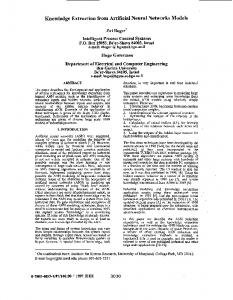
NEURAL NETWORKS A neural n~twork is a collection of simple computational elements, neurons, that are interconnected. The connections between neurons have weights attached to them. A neuron can receive inputs from other neurons or from sources outside the network, form a weighted combination of these inputs (often called NET), the weights being those assigned to the connections along with the inputs travel, and produce an output (often called OUT) that is sent to other neurons. The output may be simply the weighted combination of inputs, NET, or a nonlinear transformation of NET. This nonlinear transformation is known as a transfer, or squashing, function. The number and pattern of interconnection of the neurons in a network determine the task a network is capable of performing. The particular network form used in this chapter is known as a multilayer perceptron (MLP). A simple example is shown in Figure 6.1. There are three layers of neurons (each neuron being represented by a rectangle): an input layer, a hidden layer, and an output layer. The
P.26
Extraction of Knowledge from Accounting Reports
107
I
Figure 6.1 A Multilayer Perceptron
Input
Hidden
Output
neurons in the input layer do not perform weighting or non-linear transformation. They simply send inputs from the world outside the network to the hidden-layer neurons. In Figure 6.1, each input neuron sends its signal to each of the neurons in the hidden-layer. Each of these hidden layer neurons forms a weighted linear combination of the input values and then applies a nonlinear transformation to generate its own output. A common transfer function is the sigmoid, which generates a signal 0 s OUT s 1: OUT..
1 1 +e-NET
(3)
The signals from the hidden-layer neurons are sent to the output layer neurons. In Figure 6.1, each output-layer neuron receives input from each hidden-layer neuron. The neurons in the output layer each form linear combinations of their inputs and apply a nonlinear transforma-
P.27
108
Chapter Six
tion before sending their own signals onwards, in their case to the outside world. The sigmoid function again serves as the nonlinear transformation. The circles in Figure 6.1 do not represent neurons. They each send a signal that has a constant value of 1 along weighted connections. This weighted signal becomes part of NET for each receiving neuron. This has the effect of generating a threshold value of NET in each neuron's OUT calculation, above which OUT rises rapidly. The particular MLP shown in Figure 6.1 is capable of performing a relatively complex classification task, given that appropriate weights have been attached to the interconnections between neurons. Figure 6.2 shows a convex set of (x,y) values. The convex region is formed by the intersection of three half-spaces, each defined by a linear inequality. Each of the three linear relations that define the convex set can be represented by a linear combination of (x,y) values. Thus, each can be represented by one of the three neurons in the hidden layer of the MLP shown in Figure 6.1. Each output-layer neuron then receives over I under signals from the hidden-layer neurons, and, again by weighting and transforming the signals, carries out AND/OR operations to produce an output. In the network shown in Figure 6.1, one output neuron will produce a value close to 1 if the (x,y) pair being input lies within the convex
I
Figure 6.2 Classification Problem
y
0 X
P.28
Extraction of Knowledge from Accounting Reports
109
region. The other will produce a value close to 0 in these circumstances. The input of an (x,y) pair outside the convex region will cause a reversal of this output pattern. (Given the binary nature of the output signal required, one output neuron amid theoretically do the job. However, computational experience shows that economizing on output neurons is a mistake.) In order to model more difficult nonlinear boundaries, additional hidden layers of neurons might have to be added to the network. The problem left unresolved in the preceding description of the operation of the MLP is, where do the values of the interconnection weights come from? To carry out the classification task appropriately, each interconnection must have an appropriate weight. The network learns these weights during a training process. To build a network capable of performing a particular classification task, the following actions must be undertaken: 1. The network topology (number of layers and number of neurons in each layer) must be specified. 2. A data set must be collected to allow network training. In the example under discussion, this training set would consist of (x,y) pairs and for each pair, a target value vector (1,0) if the pair lies in the convex region of interest, (0,1) if it does not. 3. Random, small weights are assigned to each interconnection. 4. An (x,y) pair is input to the network. 5. The vector of OUT values from the output neurons is compared with the appropriate target value vector. 6. Any errors are used to revise the interconnection weights. The training set is processed repeatedly until a measure of network performance based on prediction errors for the whole training set reaches an acceptably low level. Once training has been completed, the network can be used for predictive purposes. There are two styles of training. In the first, weight updating occurs after each individual element of the training set is processed through the MLP. In the second, the entire training set is processed before updating occurs. The algorithm used to adjust interconnection weights, known as the generalized delta rule, or as the back-propagation method, is usually associated with Rumelhart et al.8 This algorithm is an enhanced version
P.29
"'···'
110
Chapter Six
of the stochastic gradient-descent optimization procedure. Its virtue is that it is able to propagate deviations backwards through more than one layer of nodes. Thus, it can train networks with one or more hidden layers. For the algorithm to work, the transfer function used in the MLP must be differentiable. Good descriptions of the algorithm exist in several sources, including Pao9 and Wasserman. 10 Wasserman's approach plays down the mathematics and emphasizes the computational steps. Minimum least-squares deviation is one possible success criterion that could be used to decide when to curtail the training process. However, there are others such as likelihood maximization. In this case the weights are adjusted to maximize the probability of obtaining the input/ output data that constitute the training set. In general, if the number of nodes in hidden layers is large compared with the number of important features in the data, the MLP behaves just like a storage device. It learns the noise present in the training set, as well as the key structures. No generalization ability can be expected in these circumstances. Restricting the number of hiddenlayer neurons, however, makes the MLP extract only the main features of the training set. Thus, a generalization ability appears. It is its hidden layers of neurons that make the multilayer perceptron attractive as a statistical modeling tool. The outputs of hidden neurons can be considered as new variables, which can contain interesting information about the relationship being modeled. Such new variables, known as. internal representations, along with the net topology, can make the modeling process self-explanatory, and so the neural network approach becomes attractive as a form of machine learning. As stated earlier, if variables are subjected to a logarithmic transformation, then a linear combination of such variables is equivalent to a complex ratio form. If the values input to an MLP are the logs of variable values, then the neurons in the (first, if there are more than one) hidden layer produce NETs that represent complex ratios. The nonlinear transformation effectively reverses the logarithmic transformation, so these complex ratios are inputs to the next layer of neurons where they are linearly combined to model the relation being investigated. The hidden layer of neurons in the MLP discussed in this chapter is, then, dedicated to building appropriate ratios. The problem of choosing the best ratios for a particular task, which has taxed so many researchers, is thus avoided. The best ratios are discovered by the modeling algorithm, not imposed by the analyst. It will be shown later
P.30
Extraction of Knowledge from Accounting Reports
111
that by using an appropriate training scheme these extended ratios can be encouraged to assume a simple and therefore potentially more interpretable form.
AN APPLICATION: MODELING INDUSTRY HOMOGENEITY The approach described above is now applied to the problem of classifying firms to industries on the basis of financial statement data. The neural network's performance is compared to that of a more traditional discriminant analysis-based approach. To ensure that the discriminant analysis exercise is more than a "straw man," an existing, reputable study based on discriminant analysis is replicated. The neural network approach is then applied using the same raw data. All companies quoted on the London Stock Exchange are classified into different industry groups· according to the Stock Exchange Industrial Classification (SEIC), which groups together companies whose results are likely to be affected by the same economic, political, and trade influencesY Although the declared criteria are ambitious, the practice seems to be more trivial, consisting of classifying firms mainly on a end-product basis. The aim here is to attempt to mimic the classification process using accounting variables. The data for exercises were drawn from the Micro-EXSTAT database of company financial information provided by EXTEL Statistical Services Ltd. This covers the top 70 percent of U.K. industrial companies. Fourteen manufacturing groups were selected according to the SEIC criteria. The list of member firms was then pruned to exclude firms known to be distressed, nonmanufacturing representatives of foreign companies, recently merged, or highly diversified. After pruning, data on 297 firms remained for a six-year period (1982-1987) and a bigger sample (502 cases) for the year 1984. The distnbution of firms by industry in this sample is shown in Table 6.1. The initial analysis of this data followed the traditional statistical modeling approach. This consisted of, first, "forming 18 financial ratios chosen as to reflect a broad range of important characteristics relating to the economic, financial and trade structure of industries." 12 Eight principal components were then extracted to form new variables. Next, these new variables were used as inputs to a multiple discriminant analysis. Only a randomly selected half of the data set was used during this estimation phase of the discriminant analysis.
P.31
112
Chapter Six
Table 6.1 Industry Groups and Number of Cases in the One-Year (1984) Data Set Group
Name
Cases
1 2 3 4 5 6 7 8 9 10
Building Mat. Metallurgy Paper, Pack Chemicals Electrical Industrial Pl. Machine Tools Electronics Motor Comp. · Clothing Wool Misc. Text. Leather Food
31
6.2
19
3.8
11
12 13
14
Percent(%)
46
9.2
45
9.0
34
6.8
17 21
3.4
79
15.7
4.2
23
4.6
42
8.4
19
3.8
30
6.0 3.2 15.9
16
80
The other half was used as a holdout sample to measure the classification accuracy of the resulting model. The exercise was repeated reversing the role of the two half data sets. Lack of consistency of results here would have raised doubts about the appropriateness of the sampling activity undertaken. A detailed description of the ratios used and the modeling procedure adopted can be found in Sundarsanam and 12 Taffler. The results of this exercise were found to be similar to those achieved by Sundarsanam and Taffler. 12 Thus, it was decided that they were an acceptable base case against which to compare the results achieved by an MLP constructed with the same data. The input data for the neural network approach consisted of eight of the accounting variables that had been building blocks for the 18 ratios previously calculated. The number eight was selected simply to mimic the number of explanatory variables in the discriminant analysis. It must be emphasized that basic accounting variables, not ratios, were used. The selected items were Fixed Assets (FA), Inventory (1), Debtors (D), Creditors (C), Long-Term Debt (DB), Net Worth (NW), Wages (W), and Operating Expenses Less Wages (EX). The variables were chosen
P.32
Extraction of Knowledge from Accounting Reports
113
to represent the key balance sheet elements and a rudimentary picture of cost structure. A logarithmic transformation was applied to these variables. Many of these accounting variables were well suited for a logarithmic transformation. However, some caused problems because of the presence of zero or negative values. In order to transform the negative values of such variables, the following rule was applied: X-> X->
log (x}, -log (lxl),
forx>O forx