as x-ray sources for l-XRF experiments and related measurements and the ... Backscatter electron micrograph of a polished section of igneous rock (150 lm in ...
X-RAY SPECTROMETRY, VOL. 26, 333È346 (1997)
Automated Segmentation of l-XRF Image Sets B. Vekemans,1 K. Janssens,1* L. Vincze,1 A. Aerts,1 F. Adams1 and J. Hertogen2 1 Department of Chemistry, University of Antwerp (UIA), Antwerp, Belgium 2 Physico-Chemical Geology, University of Leuven, Leuven, Belgium
The combined use of principal component analysis (PCA) and K-means clustering (KMC) for the segmentation and (semi-)quantitative calibration of multivariate l-XRF data sets is proposed and evaluated. The usefulness of the method is compared with that of using PCA or KMC separately by discussing image sets derived from geological and archeometric samples. ( 1997 John Wiley & Sons, Ltd. X-Ray Spectrom. 26, 333È346 (1997)
No. of Figures : 15
No. of Tables : 2
l-XRF, the microscopic equivalent of conventional (bulk) EDXRF (energy-dispersive x-ray Ñuorescence), analysis is a microanalytical technique which is still in full development.1 With respect to the variant that employs synchrotron radiation, the most signiÐcant development today and in the coming years will be the increasing availability of third-generation synchrotrons as x-ray sources for l-XRF experiments and related measurements and the consequences this will have in terms of increased sensitivity and/or lateral resolution.2 For l-XRF instruments employing laboratory-scale sources, the growing knowledge of capillary manufacture3 will also allow the extension of the analytical capabilities and of the application areas of the technique. A l-XRF image scan generates an (n ]n ]n ) col in row data cube, where n is the number ofchan channels the chan EDXRF spectrum that is collected per image pixel and n and n are the number of rows and columns in the row image. Bycolevaluating this series of (n ] n ) spectra col set row(typically either on- or o†-line,4 this extensive data 1024 ] 50 ] 50 data points) can substantially be reduced to dimensions (n ] n ] n ), where n is the col row el number of (net or gross)el elemental intensities derived from each spectrum ; in our case, n typically has values in the range 5È20. In either case, el the data cube can be considered as a multivariate data set, consisting of a number of objects (the pixels in the image) which are each characterised by a number of properties (either a complete EDXRF spectrum or vector of net elemental x-ray intensities). One of the problems associated with laboratory-scale l-XRF is the limited detectable count rate per element ; it is of the order of 10È100 times lower than what is achievable in instruments employing synchrotron radiation.5 Since during image scans usually fairly short collection times are employed per pixel (typically in the range 5È100 s), especially when one is aiming at collecting information on the distribution of trace elements in (partially) transparent samples, the photopeaks of inter-
* Correspondence to : K. Janssens. Email : koen=uia.ua.ac.be
CCC 0049È8246/97/060333È14 $17.50 ( 1997 John Wiley & Sons, Ltd.
No. of References : 30
est are often still buried in the background noise. This results in noisy images for these trace constituents. Examples are shown in Figs 1È4, where electron micrographs and l-XRF image sets of a polished rock section (Figs 1 and 2) and an archeological glass sample (Figs 3 and 4) are shown. Moreover, the noise requirements for performing precise quantitative analysis (i.e. with an uncertainty better than or equal to the accuracy o†ered by the calibration model employed) are usually more stringent than those for obtaining images from which only qualitative information on the distribution of (trace) elements on the surface of a material is to be derived. On the other hand, in most cases, the heterogeneous materials which are investigated are built up from a limited number of (quasi)homogeneous phases (see Figs 1 and 3). Elemental maps collected by means of l-XRF [or comparable methods such as electron probe x-ray microanalysis (EPXMA), l-PIXE (proton-induced x-ray emission), EELS (electron energy loss spectrometry),
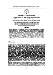
Figure 1. Backscatter electron micrograph of a polished section of igneous rock (150 lm in thickness) showing mixed mica grains (light areas), in a groundmass of microcline, a K-rich feldspar mineral (gray areas) and albite, an Na- and Ca-rich feldspar (dark areas). The small, very bright areas, inside or surrounding the Fe/Ti oxide crystals are Zn-, Cu-, Y- or Zr-rich minerals. Scale bar length, 1000 lm.
Received 9 February 1996 Accepted 20 May 1996
334
B. VEKEMANS ET AL .
Figure 2. l-XRF elemental maps obtained by scanning the sample of Fig. 1 using a 40 lm x-ray beam derived from an Mo anode operated at 40 kV. Step-size, 50 lm ; image size, 40 Ã 40 pixels or 2.00 Ã 2.00 mm ; spectrum collection time per pixel, 120 s. The maps were obtained by individual least-squares fitting of the collected spectra.
SAM (scanning Auger spectrometry) or secondary ion microscopy (SIMS)] can therefore usually be segmented into a limited number of regions, in which all pixels provide equal or similar (compositional) information, or in the multivariate sense, display a similar pattern of properties. This can clearly be seen in the elemental
Figure 3. Backscatter electron micrograph of a polished section of Roman glass showing a cut through a hemispherical corrosion growth. The complex morphology of the corrosion layer is clear. The embedding resin and the original glass are visible in the left bottom and right upper corner, respectively. Scale bar length, 100 lm. ( 1997 John Wiley & Sons, Ltd.
maps shown in Fig. 2. By segmentation of l-XRF images into a limited number of regions, it becomes possible to calculate the sum spectrum corresponding to each region (by simply adding all spectra corresponding to each of the pixels inside a region). These regionspeciÐc sum spectra feature a much lower noise level than the spectra corresponding to individual pixels and are therefore more suited for use in quantitative calculations regarding trace elements. This approach is commonly employed in l-PIXE analysis,6 but up to now its use has not been reported in the l-XRF literature. Segmentation of individual images can be done in various ways, by using e.g. edge-enhancement Ðlters or on the basis of their corresponding gray-level histograms.7,8 In the case of l-XRF (or similar) multivariate data sets it is better to employ the information in all images simultaneously during the segmentation process.8h10 This can be done by employing appropriate multivariate image processing techniques for (a) eliminating redundancies, (b) distinguishing the signiÐcant information from random noise and (c) splitting the information into mutually orthogonal (i.e. noncorrelated) components. Techniques for doing this have been reviewed recently by Bonnet8,9 and illustrated with data sets taken from electron probe microanalysis,11,12 Auger13 and EELS mapping14 and secondary ion microscopy.15 For the speciÐc case of l-XRF data sets, Cross et al.16 have described the use of principal component X-RAY SPECTROMETRY, VOL. 26, 333È346 (1997)
AUTOMATED SEGMENTATION OF l-XRF IMAGE SETS
335
Figure 4. l-XRF elemental maps obtained by scanning the sample in Fig. 3 using a 15 lm x-ray beam derived from an Mo anode operated at 45 kV. Step size, 20 lm ; image size, 50 Ã 50 pixels or 1.00 Ã 1.00 mm ; spectrum collection time per pixel, 60 s.
analysis (PCA) for collinearity removal and dimensionality reduction. By manually grouping pixels in the space of the resulting principle components (see below), semi-automated or supervised image segmentation was shown to be feasible for data sets in which a limited number of three principal components were present. This approach to segmentation is termed interactive correlation partitioning (ICP).12 In this paper, two alternative approaches to image segmentation are compared which can be automated to a higher degree than the procedure described by Cross et al.16 and which (as a result) can also be easily applied to data sets in which more than three principal components are present. With this type of procedure, automated correlation partitioning (ACP) then becomes possible.9 Also, the usefulness of these segmentation procedures for extracting from a l-XRF image data set a small number of region-speciÐc sum spectra is evaluated. Instead of attempting to reduce the dimensionality of the (n ] n ] n ) data set by looking for collinearity col row between el (or covariance) the various elemental signals within the images (as is done in PCA), the Ðrst ( 1997 John Wiley & Sons, Ltd.
approach performs image segmentation by considering all (n ] n ) pixels as objects characterized by a vectorcolof n row properties (a multivariate “ÐngerprintÏ) and by using aelsuitable clustering algorithm to generate a limited number of pixel groups having similar Ðngerprints. Since in a l-XRF image the number of pixels usually is of the order of or larger than 1000, not all clustering algorithms are suitable for this work. In this paper, the K-means clustering (KMC) algorithm was employed since it is a standard and easily understandable clustering procedure, well suited for processing the large data sets discussed here. The second approach is a combination of PCA and K-means pixel clustering : in a Ðrst step, the eigenvalues and principal component images (or eigenimages) of the original data set are calculated using PCA ; second, a limited number of these eigenimages are used as input to the KMC algorithm, allowing the original elemental maps to be segmented. In what follows, after a brief description of the experimental l-XRF set-up employed and of the mathematical principles behind some of the above-mentioned multivariate pattern recognition techniques, the X-RAY SPECTROMETRY, VOL. 26, 333È346 (1997)
336
B. VEKEMANS ET AL .
working principle of both segmentation approaches are explained by means of (the relatively simple) data set shown in Fig. 2, corresponding to the geological sample in Fig. 1. To illustrate the practical usefulness of both approaches for segmentation and (semi)quantitative l-XRF analysis of truly multi-component materials (i.e. consisting of more than three phases) such as the corroded glass sample shown in Fig. 3, the analysis of the data set shown in Fig. 4 will be discussed.
EXPERIMENTAL The l-XRF set-up used to collect the data sets shown in Figs 2 and 4 consists of a Siemens M18XHF rotating anode generator, various glass capillaries of di†erent dimensions and shape (conical and straight), an XY Zh sample translation/rotation stage, an optical microscope and an Si(Li) detector. Details of the set-up and of the capillaries employed are given elsewhere.17 The x-ray source can be operated up to a maximum power of 18 kW (400 mA/45 kV). The x-ray emerging from the anode tower are focused by a glass capillary mounted on a four-axis gimbal lens holder which allows for a precise positioning of the former. The sample stage consists of three linear stages (100 mm travel, 1 lm step size) which are mounted in an XY Z geometry and rotation unit (0.01¡ angular step). Samples are mounted directly on the rotation table, allowing the sample to be independently translated and rotated from a “measuringÏ position (in front of the capillary tip) to a “viewingÏ position in the focal plane of the optical microscope. The latter is equipped with 4 ] , 10 ] and 20 ] longworking distance objectives (2 cm) and a colour video camera. Fluorescent radiation is detected with an 80 mm2 Si(Li) detector, which is shielded by a 5 mm diameter Mo aperture. Spectrum acquisition is performed with a PC plug-in MCA card ; the PC also handles the coordinated movement of the motors. As a result of intimate integration of the spectrum acquisition, sample scanning and the spectrum evaluation software, during most of the acquisition procedure, quasi-parallel data acquisition and spectrum evaluation are possible.18
operates on (two-dimensional) data matrices, threedimensional (n ] n ] n ) l-XRF data sets Ðrst row col el need to be unfolded to two-dimensional (n ] n ) pix el matrices. [This procedure simply involves the reordering of the (n ] n ) pixel values that constitute the row col mth x-ray map into a vector V of length n \ n m pix row ] n ; the resulting set of vectors MV N forms an (n col m pix ] n ) data matrix V]. PCA achieves its goal by replael cing the original variables of this data matrix (in this case, the chemical elements) by mutually orthogonal (i.e. uncorrelated) linear combinations of the latter. These linear combinations are called principal components (PC). In the hyperspace (of dimension n ) subtended by el the original variable axes, in which each of the (n row ] n ) pixels (index i) can be represented by a point at a col location deÐned by its intensity V in each of x-ray ij maps (index j), the PCs are a new set of mutually orthogonal axes that are better suited to describe the structure of the clouds of data points (the pixels) which are present in this space (see Fig. 5). The projection of the ith data point/pixel on the kth PC axes is called the score t of that pixel. Sinceik the PCs are linear combinations of the original variables, the scores can be calculated using nel t \ ;p V jk ij ik j/1 or in matrix notation T \ VP, where T is the (n ] n ) pix (nel score matrix and P is called the loading matrix el ] n ) ; p expresses the contribution of the jth original el ij variable to the kth principal component. The set of loading vectors MP N that constitute P are calculated in k three steps : 1. First, the data matrix V is optionally scaled and/or centered. This yields the data matrix Z. This data pretreatment in our case usually involves dividing each vector V by the square root of its mean value ; m can be considered as a way of weighthis scaling step ing the contribution of each image using the uncertainty of the average intensity as weight ; an alternative is to subtract from each vector its mean value and to divide the result by its standard deviation. Both of the above pretreatment approaches
MATHEMATICAL BACKGROUND
Principal component analysis A l-XRF data set consisting of a series of x-ray maps, each corresponding to one chemical element, may contain images which are highly correlated (see Fig. 2, Ti, Mn and Fe images) and some images which do not convey any information (see Fig. 4, Si, S and Cl images). PCA is a multivariate statistical technique which is aimed at highlighting the varianceÈcovariance structure of experimental multivariate data sets, essentially through reduction of the dimensionality of the data.19,20 Since PCA is a mathematical procedure that ( 1997 John Wiley & Sons, Ltd.
Figure 5. The principle of principal component analysis : in the hyperspace of the original variables, new principal component axes are defined, which are better suited to describe the variation in the set of data points considered. X-RAY SPECTROMETRY, VOL. 26, 333È346 (1997)
AUTOMATED SEGMENTATION OF l-XRF IMAGE SETS
donÏt directly have a physical meaning but are based on statistical considerations ; another way is to divide each vector (corresponding to the x-ray map of a particular chemical element) by the appropriate thinsample sensitivity coefficient (expressed, e.g., in counts ng~1) in order to perform the multivariate data reduction in concentration space rather than in x-ray intensity space. 2. The matrix Z is multiplied with its transpose Zº (yielding an (n ] n ) real symmetric matrix ZºZ) el to tridiagonal el which is reduced form by using HouseholderÏs method.21,22 3. The n eigenvalues and eigenvectors of this matrix el are calculated using the QL algorithm.22 These eigenvectors are also called the loading vectors MP N ; k since the eigenvalue e that corresponds to each k eigenvector is proportional to the variance explained by that PC, the loading vectors are sorted accordingly. Once the loading vectors are known, the score matrix can be calculated as detailed above. By refolding the set of score vectors MT N that constitute T, a set of n score el images is obtained,k also called principal component or eigenimages. By this transformation, all pixels which were originally characterized by a vector of n x-ray el array map intensities are now redeÐned in terms of an of n score values, as illustrated graphically in Fig. 5. el the Ðrst few PC images (associated with large Usually eigenvalues) will show a high contrast and a low noise level while the remaining ones will convey less and less information (see below). The eigenvalue e corresponding to the kth score image (or loadingk vector) is a measure of the fraction of the total variance in the data set which is explained by that principal component ; usually, one plots CV E \ e /&e (CV E \ contribution k kagainst k to the variance explained) the PC index to obtain an idea how many of the PCs are necessary to explain most of the variance (say, 90%) in the data set [see Fig. 7(a)].
The K-means clustering algorithms All clustering methods employ a means of calculating the degree of similarity (or distance in property space) between two of the objects to be clustered. In our case, the objects are pixels (index i) and their properties q ij (index j) are either the net x-ray intensities derived from the spectrum of pixel i (q 4 V ) or the score values of ij PCijaxes (q 4 t ). The simithat pixel on the equivalent larity measure between two pixels iij andij k can be expressed as an Eucledian distance d : ik N N d \ ; w (q [ q )2 ; w j ij kj j ik j/1 j/1 where N is the total number of properties used for clustering and w is the weight of the jth property. j The K-means clustering algorithm is an iterative procedure that derives its name from the fact that it assumes the Ðnal number of objects classes (or pixels clusters or image segments) to be known a priori and equal to K. Each iteration is composed of three steps :
S
( 1997 John Wiley & Sons, Ltd.
N
337
1. calculate the location of centers of the K clusters in the N-dimensional space using 1 qcenter \ ; q kj ij N k i|k where k is now the cluster index and j the property index while the summation runs over all pixels i belonging to cluster k (N in total) ; k 2. reclassify all pixels in all clusters according to a nearest-neighbor strategy : pixel i is associated with cluster k if its distance to the cluster center d is the ik smallest, d \ d for all other cluster centers k@ difik ik@ ferent from k ; 3. if no pixel has changed cluster in step (2) compared with the situation in step (1), stop ; otherwise go to step (2). As initial locations of the K cluster centers, Bonnet9 suggests using (a) for the Ðrst cluster center the object which has the largest distance from the center of gravity of all objects, (b) for the second cluster center the object which is the farthest from cluster center 1 and (c) for the remaining (K [ 2) cluster centers the objects which are the farthest from the previously established cluster centers (see Ref. 9 for details). Obviously, the way of calculating the weights w directly inÑuences the “distanceÏ between two objectsj and therefore also the result of the entire clustering procedure.
RESULTS AND DISCUSSION
The granite data set Figure 1 shows an electron micrograph of an 150 lm thick polished section of igneous rock and in Fig. 2 the elemental maps obtained by Ðtting all 40 ] 40 spectra are shown. The Z (atomic number) contrast in the backscattered electron image, together with the elemental maps in Fig. 2, immediately shows that there are several distinct phases in this material : (a) the three square-like crystals contain a high weight percentage of Fe and Ti oxides and feature a high backscatter intensity in Fig. 1 ; several small areas feature an even higher backscatter intensity : one is near the right-upper face of the topmost crystal and some are inside (near the center) of the bottom crystal ; some of these small areas contain substantial amounts of either Zr, Y or Zn ; (b) a phase of intermediate backscatter intensity and mean Z (atomic number) interspersed with darker exsolution lamellae, called microcline, a K-rich feldspar ; and (c) the albite phase, (an Na- and Ca-rich feldspar mineral) shown the darkest in Fig. 1. The elemental maps in Fig. 2 were obtained with a 40 lm diameter x-ray beam and consequently the lamellae in the microcline phase are not resolved. Next to the major elements of the di†erent phases (K, Ca, Ti, Mn, Fe), also meaningful images on (trace) constituents such as Zn, Rb, Sr, Y and Zr are shown, in addition to the maps of the Compton and Rayleigh scatter peak intensities. From the Y and Zr maps, it is clear that these elements appear almost X-RAY SPECTROMETRY, VOL. 26, 333È346 (1997)
B. VEKEMANS ET AL .
338
exclusively in the small areas mentioned above. The Cu map (not shown) does not provide such a clear picture because of di†raction peaks overlapping with the characteristic lines. Di†erentiation of the few Y- and Zr-rich pixels from the rest of the image is straightforward (e.g. by threshholding) and will not be addressed here in order to simplify this Ðrst data set somewhat (see later). This type of material is similar to that described by Cross et al.16 In Fig. 6, the principal component images resulting from PCA analysis of the data in Fig. 2 (using the maps of K, Ca, Ti, Mn, Fe, Zn, Rb and Sr as starting data) are shown. The loadings of the original variables are given in Table 1, together with the CV E of each PC. In Fig. 7(a), the CV E of each PC is plotted ; clearly the Ðrst three PCs explain 90% of the total variance in the data set. The most meaningful contrast between the various phases is also visible in images
Figure 6. Score images obtained by PCA the x-ray maps in Fig. 2.
PC1ÈPC3 : PC1 more or less resembles the inverse of the K-map in Fig. 2, although the distinction between the Fe-rich and -poor areas is the most striking ; PC3 emphasizes the Zn-rich pixels ; in PC2, the distinction between K-rich and -poor areas is apparent, while the Zn-rich pixels are also visible. When the scores of all pixels on the Ðrst and second principal component axes are plotted in a scatter diagram as shown in Fig. 7(b), a clear visual distinction can be made between three pixel clusters. As pointed out by Trebbia et al.,23 the fact that these three groups can so easily be separated and in the PC1ÈPC2 plane form the vertices of an (almost) equilateral triangle is an indication that this material is mainly composed of only three mineral species (see Fig. 2 in Ref. 22 for details). Figure 7(c) shows the PC1ÈPC2 loading plot of the original variables, i.e. the chemical elements. In some cases, the loading and score plots may be superimposed to facilitate the interpretation of the clusters (or other structures) which are visible in the score plots in terms of the original variable. In principle, this is only possible when a variant of PCA called “correspondence analysisÏ24 is employed ; this involves double (i.e. row and column) scaling and centering of the original data matrix prior to the decomposition. As explained by Wold et al.,24 however, by appropriate axes scaling of the loading or score plots with respect to each other (see Ref. 24 and references cited therein for details) the same e†ect may be achieved with ordinary PCA as well. Hence it is possible qualitatively to associate (a) with the topmost cluster (] symbols) [top left quadrant in the score plot of Fig. 7(b)] a high K signal [top left quadrant in the loading plot of Fig. 7(c)], corresponding to the K-feldspar phase, (b) with the lower left cluster (\ symbols) a high Fe signal (bottom left quadrant), corresponding to the mica/biotite mineral grains, and (c) with the lower right cluster (diamond symbols) a high Ca signal which corresponds to the plagioclase phase (in view of the in-air operation of the spectrometer, the Na signal is not detectable). Also, observe the location of Rb, Sr and Ti/Mn relative to K, Ca and Fe, respectively, in Fig. 7(c), indicating strong collinearity between K/Rb, Ca/Sr and Ti/Mn/Fe. The Zn signal is not associated with one of these groups and occupies an intermediate position between the Fe and Ca group in Fig. 7(c) ; in the score plot of Fig. 7(b), a few “outlierÏ pixels (triangle symbols) are located in approximately that position also.
Table 1. Loading of the original variables on the principal components found for the granite data set [ see Fig. 7(b) and (c) ] Original variable
PC1
PC2
PC3
PC4
PC5
PC6
PC7
PC8
K Ka Ca Ka Ti Ka Mn Ka Fe Ka Zn Ka Rb Ka Sr Ka CVE a (%)
É0.32 0.33 É0.39 É0.40 É0.40 É0.12 É0.38 0.37 60.9
0.50 É0.42 É0.38 É0.35 É0.35 É0.29 0.27 É0.16 16.4
É0.08 0.12 0.17 0.17 0.15 É0.95 É0.02 0.02 11.4
É0.48 É0.36 É0.03 É0.10 É0.05 É0.04 É0.38 É0.69 4.7
0.02 É0.70 0.19 0.06 0.05 É0.02 É0.04 0.K55 3.7
0.63 0.27 0.18 0.00 É0.03 0.01 É0.67 É0.22 2.3
É0.05 0.04 0.70 É0.69 É0.07 0.00 0.16 0.01 4
0.06 0.00 É0.33 É0.45 0.82 É0.01 É0.08 0.03 1
a CVE ¼ contribution of variance explained (see text).
( 1997 John Wiley & Sons, Ltd.
X-RAY SPECTROMETRY, VOL. 26, 333È346 (1997)
AUTOMATED SEGMENTATION OF l-XRF IMAGE SETS
339
Figure 7. Scatter diagrams corresponding to the data shown in Figs 2 and 6 : (a) CVE (contribution of variance explained) of each principal component, (b) score and (c) loading plots in the PC1–PC2 plane.
It is clear that by means of Fig. 7(b), the cluster separation can easily be done manually. The symbol assignment in Fig. 7(b), however, was obtained by using the PC1 and PC2 images as input to the K-means clus( 1997 John Wiley & Sons, Ltd.
tering algorithm. As already mentioned, when starting the KMC algorithm, one needs to specify a priori the desired number of clusters. When segmentation into four clusters is desired, the results shown in Figs 7(b) X-RAY SPECTROMETRY, VOL. 26, 333È346 (1997)
340
B. VEKEMANS ET AL .
and (c) and 8 are obtained : next to the K-, Ca- and Fe-rich clusters corresponding to the microcline, albite and opaque mineral phases, respectively, a small fourth cluster of the above-mentioned outliers pixels is distinguished which is associated with a high Zn signal. Approximately the same clusters as shown in Fig. 8 can be obtained by directly applying the K-means algorithm to the data of Fig. 2, i.e. without the PCA step in between. Meaningful results are only obtained, however, when (a) one manually selects the images showing a high contrast and having low noise (i.e. the K, Ca and Fe images) and (b) when the x-ray intensities are scaled by dividing through their standard deviation within each image. Other types of data pretreatments (such as taking the logarithm or the square root of the data) are also possible but result in either non-meaningful or non-contiguous segmentation. Also, the manual preselection of images for use as input to the clustering algorithm has a strong inÑuence on the results of the clustering procedure. As an example, Fig. 9 shows the results of clustering the eight maps which were previously employed as input for the PCA procedure and by requesting the KMC procedure to divide the pixels into four [Fig. 9(a)] and six [Fig. 9(b)] clusters. It appears that in this case, at least six clusters need to be considered in order to obtain results similar to those obtained with PCA pretreatment (see Fig. 8). The distinction between the albite and microcline phases is only made after a number of outlier pixels, associated with high Ca and Zn intensities, have been separated into clusters of their own. In all cases described above, image scaling by the standard deviation of the image intensity was performed. The e†ect of various ways of data pretreatment on the Ðnal segmentation results clearly needs to be studied further, but is beyond the scope of this paper. For this case, it can be concluded that the use of the PCA pretreatment prior to the K-means clustering is not really necessary and can be replaced by simpler pretreatments operations ; the PCA pretreatment does allow one to limit the user intervention to determining (if necessary by trial and error) the number of relevant
Figure 9. Compound segmentation masks obtained by K -means clustering of the original data in Fig. 2, using the eight maps previously employed as input for PCA and by requesting grouping into (a) four and (b) six clusters.
PCs that will be used as input data to the clustering procedure. However, both PCA plus manual cluster selection or the KMC procedure alone can (after some experimentation) provide adequate results also.
The Roman glass data set Figure 8. Individual and compound segmentation masks obtained by K -means clustering on the first three score images shown in Fig. 6. ( 1997 John Wiley & Sons, Ltd.
The usefulness of combining PCA and KMC is clearer when processing the x-ray images derived from the corroded glass sample shown in Figs 3 and 4. When glass X-RAY SPECTROMETRY, VOL. 26, 333È346 (1997)
AUTOMATED SEGMENTATION OF l-XRF IMAGE SETS
Figure 10. Score images obtained by PCA of the elemental maps in Fig. 4.
is buried in soil for extended periods of time, owing to di†usion of cations out of the glass and their replacement with protons from the groundwater, a gel layer is formed. This leached layer can become extensive (up to a few 100 lm in thickness) and, since it is depleted in (voluminous) cations, has di†erent macroscopic properties from the original glass. One of the properties is the thermal expansion coefficients of the layer ; changes in temperature can therefore induce stress between the underlying glass body and the leached layer, causing cracks to appear through which water can again attack the glass, form a new leached layer, etc. Corrosion also can proceed from small air bubbles or impurities in the glass and create the hemispherical corrosion morphology shown in Fig. 3. Since the leached layer, when initially formed, is poor in cations, other ionic species (such as Mg, Mn, Fe, Cu, Zn and Ni), which are dissolved in the water surrounding the glass, can easily penetrate into the leached layer and become enriched in concentration in certain layers. Depending on the electrochemical potential and the pH of the environment, also precipitation of, e.g., MnO can take place inside 2 the corroded layer or in the cracks that have formed. All these chemical and physical changes in the glass Ðnally lead to a multi-phase material of complex morphology which can be conveniently studied by means of l-XRF.25 For the measurements, a piece of Roman glass was embedded in orthodontic resin, cut and polished to reveal the cross-section shown in Fig. 3. As shown in Fig. 4, the resulting elemental maps (50 ] 50 pixels) show a complex picture : next to the Mn-rich areas where precipitation occurred, several bands of di†erent composition can be distinguished. The top layer corre( 1997 John Wiley & Sons, Ltd.
341
sponds to the original glass (high Ca signal) while the bottom layer is the embedding resin. Many of the trace element maps (e.g., Ti, Cr, Ni, Zn, Br, Pb) however, have a noisy appearance. In Fig. 10, the Ðrst nine principal component images, resulting from PCA processing of all the original maps of Fig. 4, are shown. Clearly, images PC1ÈPC7 are contrast-rich whereas in the remaining PCs noise dominates the pictures ; together, PC1ÈPC7 explain more than 99% of the variance in the data. In Fig. 11, some score and loading scatter plot pairs are given. In contrast with the previous case, it is now impossible to Ðnd a pair of principle components where all pixel clusters can be straightforwardly separated. As can be seen in the Fig. 11(a), some pixel clusters [associated with a high Mn signal ; see Fig. 11(b) are spread out in the PC2ÈPC3 plane whereas several others are located on plane(s) perpendicular to the former such as the PC3È PC4 plane [Fig. 11(c)]. Although the use of 3D scatter diagrams would simplify manual interpretation in this case (see Bright19 for examples), manual cluster separation appears to be difficult here in one step, although it probably is possible if the results of several subsequent selections (in various 2D or 3D cross-sections of the PC hyperspace) were combined. By using the seven meaningful PCA images as input for the KMC procedure, the pixel grouping indicated in Fig. 11(a) and (c) was obtained. The resulting segment masks and sum spectra are shown in Figs 12 and 13. As could already be expected from the association of, e.g., cluster 7 [circle symbols in Fig. 11(a) and (c)] with a high Compton scatter signal [see Fig. 11(b) and (d)] and with no clear association to any of the elemental signals, this image segment corresponds to the embedding resin ; accordingly, the corresponding cluster sum spectrum (Fig. 13) shows (almost) only background and a high Compton/Rayleigh ratio. On the other hand, sum spectrum 2 shows abundant Ca, Mn and Fe signals and especially a clear Sr peak and a much lower Compton/ Rayleigh ratio ; this image segment corresponds to the original glass and is clearly separated from the others in the PC3ÈPC4 plane [see Fig. 11(c), \ symbols, and (d)]. Cluster 3 shows a similar pattern but shows clear Cu and Bi signals ; this probably corresponds to a Bi-rich precipitate in the crack between the original glass and the corroded layer. Clusters 6 and 9 contain only a few pixels of a Bi “hot spotsÏ but essentially show the same pattern. The rest of the clusters appear much less well deÐned in the scatter plots shown in Fig. 11, although in other plots (not shown here), e.g. clusters 4 and 1 (respectively the MnO precipitation area and the phase 2 Mn and Fe signals) and clusit originated fromÈhigh ters 8 and 10 (top part of the leached layer, parallel with the surface and precipitate crust formed on top of the surface, probably consisting of predominantly gypsum, CaSO É 2H O, and syngenite, K SO É CaSO É H O, 4 a high 2 2 with 4 4 2 yielding Ca signal associated a relatively low Sr signal) can be easily distinguished from the rest. It should be noted that also in this case, it was possible to obtain about the same segmentation and corresponding sum spectra by using KMC alone. These results, however, were only obtained after a fairly extensive trial-and-error procedure, during which various data pretreatments and di†erent sets of starting images X-RAY SPECTROMETRY, VOL. 26, 333È346 (1997)
342
B. VEKEMANS ET AL .
Figure 11. Scatter diagrams corresponding to the data shown in Figs 4 and 11 : (a, b) score and loading plots in the PC2–PC3 plane ; (c, d) in the PC3–PC4 plane.
were employed. When all the images in Fig. 4 are involved in the KMC procedure and image centering and scaling are performed (making the noisy images as important as the others), non-contiguous segments are obtained ; also, the resin phase did not end up in a cluster of it own. When the centering/scaling was omitted, subtle di†erences among clusters (e.g. the K/Ca ratio in clusters 8 and 10) were not recognized while others segments were divided into several subparts (e.g. cluster 4) that featured very similar sum spectra. In order to obtain approximately the same results as ( 1997 John Wiley & Sons, Ltd.
shown in Figs 12 and 13, it was found necessary to use only the K, Ca, Ti, Mn, Fe, Cu, Sr, Bi, Rayleigh and Compton maps, i.e. to eliminate manually the images with high noise content, and to scale them prior to clustering by division through their standard deviation. One can conclude again that the use of the PCA pretreatment allows for more rapid processing of the data set by elimination of noise and reduction of dimensionality prior to the clustering. Comparison of the x-ray maps of Fig. 4 and of the sum spectra in Fig. 13 indicates that, although some of X-RAY SPECTROMETRY, VOL. 26, 333È346 (1997)
AUTOMATED SEGMENTATION OF l-XRF IMAGE SETS
343
Figure 11. Continued
the x-ray maps show an excessively noisy distribution, most of the sum spectra feature (sometimes weak but) predominantly noise-free photopeaks, allowing the corresponding major and trace constituents to be determined with an uncertainty which mainly derives from the errors in the calibration model and not from counting statistics. By employing a detailed simulation model for predicting the spectral response of the l-XRF spectrometer in combination with a fundamental parameter code,26,27 the sum spectra were converted into concentration data. In this case, this process can only be done semi-quantitatively because of the complex (and largely unknown) morphology and depth ( 1997 John Wiley & Sons, Ltd.
of the various layers which constitute the hemisphere shown in Fig. 3. The issue of reliably quantifying l-XRF data obtained from heterogeneous samples is a complex one and is being addressed by us and by others elsewhere.28h30 Since the sampling depth of the various elemental signals in the glass and the various phases in the corrosion layer vary between 10 and [100 lm, an error in the thickness estimation of the phase involved directly propagates to the estimated concentration. To provide an idea on the magnitude of the errors being made, in Fig. 14, the variation in obtained quantitative data with assumed sample thicknesses in the range 10È 1000 lm is plotted for the case of cluster 4 (see Figs 12 X-RAY SPECTROMETRY, VOL. 26, 333È346 (1997)
B. VEKEMANS ET AL .
344
Figure 12. Individual and compound segmentation masks obtained by KMC on the first seven score images shown in Fig. 10.
and 13). Clearly, for elements such as Ca, all layer thicknesses above 50 lm provide the same concentration, since the layer acts as an inÐnitely thick sample for their characteristic radiation ; for the Sr and Br radiation, however, the correct choice of layer thickness is critical and, in this case, leads to a larger uncertainty on the concentration of these elements. In Table 2, the results of these (semi-quantitative calculations are listed for
some of the phases shown in Fig. 12 and for each segment the assumed average thickness of the corresponding phase is also mentioned. These thicknesses d were estimated by considering the dimensions r and r of the layers in the picture shown in Fig.0 3 and1 assuming the layers to bend spherically below the surface, as shown in Fig. 15. Based upon EPXMA analysis of the original glass (see Ref. 25, Table 2), for all
Table 2. Semi-quantitative analysis results obtained by quantifying some of the cluster sum spectra shown in Fig. 13 Cluster No. Element
1
2
3
4
5
8
K (%) Ca (%) Ti (ppm) Cr (ppm) Mn (%) Fe (%) Ni (ppm) Cu (ppm) Zn (ppm) Br (ppm) Sr (ppm) Pb (ppm) Bi (ppm) Depth (lm)
0.87 0.38 500 35 0.71 0.35 15 380 120 35 150 70 95 310
0.37 3.12 240 5 0.42 0.18 5 30 40 5 300 45 30 400
0.51 2.39 330 20 0.38 0.26 ÄMDL 240 85 15 370 80 700 150
0.88 0.52 180 50 6.72 0.44 95 390 145 45 320 165 160 200
0.99 0.36 570 15 0.13 0.40 10 60 60 25 80 40 40 600
0.83 0.74 400 10 0.78 0.31 25 90 72 20 120 70 70 150
( 1997 John Wiley & Sons, Ltd.
X-RAY SPECTROMETRY, VOL. 26, 333È346 (1997)
AUTOMATED SEGMENTATION OF l-XRF IMAGE SETS
345
Figure 15. Drawing of the approximative scheme which was used to estimate the thickness of the various layers in the hemispherical corrosion body shown in Fig. 3.
phases except the original glass, a “dark matrixÏ consisting of SiO was assumed ; in the case of the original 2 glass, a mixture of SiO (70% w/w) and Na O (17% 2 2 w/w) was employed.
CONCLUSIONS
Figure 13. Image and cluster sum spectra corresponding to the clusters shown in Fig. 12.
Figure 14. Variation of the apparent concentration of Ca, Cu, Sr and Br in the phase corresponding to cluster 4 (see Fig. 12) depending on the assumed average thickness of the layer.
By means of two l-XRF data sets derived from geological and archeometric materials of di†erent complexity, the possibility of using the KMC algorithm for automated image segmentation has been explored. When the clustering algorithm is directly applied to the net x-ray maps, care must be taken that only images with high contrast/low noise content are used and that they are appropriately scaled relative to each other. We Ðnd that division of each image through the standard deviation of the pixel intensities yields satisfactory results. An alternative pretreatment method which simultaneously takes care of scaling and the image selection/noise removal problem is to calculate, via PCA, the principal component images of the set of original x-ray maps and to use the meaningful PC images as input to the clustering procedure. This combination of PCA and KMC requires minimal user input and is able to perform meaningful segmentation of l-XRF image sets. The resulting sum spectra associated with each image segment (and the corresponding compositional information) simpliÐes the interpretation of the measurements and can be used as input for (semi-)quantitative calculations.
REFERENCES 1. A. Rindby, X -Ray Spectrom . 22, 187 (1993). 2. J. V. Smith, Conf . Ser . Inst . Phys . 160, 605 (1992). 3. D. Carpenter (Ed.), this Special Issue of X -Ray Spectrom . 26 (1997). 4. B. Vekemans, K. Janssens, L. Vincze, F. Adams and P. Van Espen, X -Ray Spectrom . 23, 278 (1994). ( 1997 John Wiley & Sons, Ltd.
5. K. Janssens, L. Vincze, B. Vekemans, A. Rindby, F. Adams, K. Jones, A. Knochel, P. Engstrom and D. Carpenter, X -Ray Spectrom . submitted for publication. 6. E. Svietlicki, N. P. Larsson and C. Yang, Nucl . Instrum . Methods Sect . B 77, 195 (1993). 7. J. C. Russ, The Image Processing Handbook . CRC Press, X-RAY SPECTROMETRY, VOL. 26, 333È346 (1997)
B. VEKEMANS ET AL .
346
8. 9. 10. 11. 12. 13. 14. 15. 16. 17. 18. 19. 20.
Boca Raton, FL (1994). N. Bonnet, Microchim . Acta 120, 195 (1995). N. Bonnet, Ultramicroscopy 57, 17 (1995). P. Geladi, Microchim . Acta 120, 211 (1995). D. S. Bright, D. E. Newbury and R. Marinenko, Microbeam Anal . 18 (1988). J. M. Paque, R. Browning, P. L. King and P. Pianetta, Microbeam Anal . 19 (1990). M. Prutton, M. El Gomati and P. G. Kenny, J . Electron Spectrosc . Relat . Phenom . 52, 197 (1990). C. Jeanguillaume, J . Microsc . Spectrosc . Electron . 10, 409 (1985). P. Van Espen, G. Janssens, W. Vanhoolst and P. Geladi, Analusis 20, 81 (1992). B. Cross, R. D. Lamb, S. Ma and J. M. Paque, Adv . X -Ray Anal . 35, 1255 (1992). K. Janssens, B. Vekemans, F. Adams, L. Vincze and A. Rindby, Spectrochim . Acta , Part B B51, 1661 (1996). K. Janssens, B. Vekemans, F. Adams, P. Van Espen and P. Mutsaers, Nucl . Instrum . Methods , Sect . B B109/110, 179 (1996). D. Bright, Microbeam Anal . 4, 151 (1995). P. Geladi and B. R. Kowalski, Anal . Chim . Acta 185, 1 (1986).
( 1997 John Wiley & Sons, Ltd.
21. R. A. Johnson and D. W. Wickern, Applied Multivariate Statistical Analysis , 2nd ed. Prentice Hall, Englewood Cliffs, NJ (1988). 22. W.H. Press, S. A. Teukolsky and W. T. Vetterling, Numerical Recipes in C : The Art of Scientific Computing , 2nd ed. Cambridge University Press, Cambridge (1992). 23. P. Trebbia, J. M. Wulveryck and N. Bonnet, Microbeam Anal . 4, 85 (1995). 24. S. Wold, K. Esbensen and P. Geladi, Chemolab . 2, 37 (1987). 25. K. Janssens, A. Aerts, L. Vincze, F. Adams, C. Yang, R. Utui, K. Malmqvist, K. W. Jones, M. Radkte, S. Garbe, F. Lechtenberg, A. Kno chel and H. Wouters, Nucl . Instrum . Methods , Sect . B B109/110, 690 (1996). 26. L. Vincze, K. Janssens and F. Adams, Spectrochim . Acta , Part B 48, 553 (1993). 27. K. Janssens, L. Vincze, P. Van Espen and F. Adams, X -Ray Spectrom . 22, 234 (1993). 28. M. Lankoszj and P. A. Pella, X -Ray Spectrom . 23, 169 (1994). 29. P. Voglis and A. Rindby, J . Trace Microprobe Tech . 13, 177 (1995). 30. K. Janssens, L. Vincze, B. Vekemans, A. Aeuts, F. Adams, K. W. Jones and A. Kno chel, Microchimica Acta 13, 87, (1996).
X-RAY SPECTROMETRY, VOL. 26, 333È346 (1997)