Bayesian approach to estimation of the map of dark current in wavelet domain J. Švihlík*, M. Řeřábek, P. Páta Czech Technical University in Prague, Faculty of Electrical Engineering, Department of Radioelectronics, Technická 2, 166 27, Prague 6, Czech Republic a
ABSTRACT This paper deals with advanced methods for elimination of the thermally generated charge in the astronomical images, which were acquired by Charged Coupled Device (CCD) sensor. There exist a number of light images acquired by telescope, which were not corrected by dark frame. The reason is simple the dark frame doesn’t exists, because it was not acquired. This situation may for instance come when sufficient memory space is not available. There will be discussed the correction method based on the modeling of the light and dark image in the wavelet domain. As the model for the dark frame image and for the light image the generalized Laplacian was chosen. The models parameters were estimated using moment method, whereas an extensive measurement on astronomical camera were proposed and done. This measurement simplifies estimation of the dark frame model parameters. Finally a set of the astronomical testing images were corrected and then the objective criteria for an image quality evaluation based on the aperture photometry were applied. Keywords: dark frame correction, wavelet transform, image model, Bayesian estimator
1. INTRODUCTION There exist many astronomical observatories (see section 2) on the world. These observatories produces huge amount of scientific image data, which are investigated by several researchers. Unfortunately, a large number of scientific image need sufficient storage disk space, even these are suitably compressed. For instance, when the images of night sky acquired by CCD (Charge Coupled Device) sensor are considered then it is necessary to acquire except light image also among others correction dark frame. This image serves for the thermally generated charge elimination, which are made by subtraction of the dark frame from the light image. The thermally generated charge can be also eliminated by nonlinear median filtering, but as was mentioned above this method is not so satisfactory. Method described in this paper allows correcting light image directly and among others saves memory space.
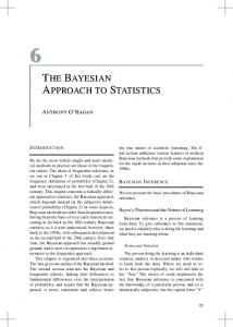
Fig. 1. The 1m11.01.dat image, exposure time = 300 sec, CCD temperature = 4.21 °C.
*
[email protected]; phone +420 2 2435 2113; fax +420 2 3333 9801
Advanced Software and Control for Astronomy II, edited by Alan Bridger, Nicole M. Radziwill Proc. of SPIE Vol. 7019, 701932, (2008) · 0277-786X/08/$18 · doi: 10.1117/12.787805
Proc. of SPIE Vol. 7019 701932-1 2008 SPIE Digital Library -- Subscriber Archive Copy
2. IMAGE DATA
Autocorrelation
Two 16 bits scientific astronomical images (fits and dat format) were chosen for the simulations. FITS (Flexible Image Transport System) is primarily designed to store scientific data sets. These scientific analysed data has been taken during work of the international (Czech-Spanish) experiment BOOTES (Burst Observer Optical Transient Exploring System). The BOOTES1 has been in service since 1998 as the first Spanish robotic telescope for the sky observation. This system is one of the three similar systems in fully operation in the world. The main aim of the project is an observation of the extragalactic objects and detection of a new optical transient (OT) of gamma ray burst (GRB) sources. An example of the light image is depicted in the Fig. 1. An image behavior can be described using autocorrelation function. There is a typical autocorrelation function of the astronomical images in the Fig. 2, where can be seen that the shape of this autocorrelation function is quite slim. So, this means that the astronomical images are noise similar. The z axis shift of the autocorrelation denotes the direct-current component.
1
0.5
0 50
50
0
Shift
0 -50
-50
Shift
Fig. 2. The 1m11.01.dat image autocorrelation function.
3. DISCRETE WAVELET TRANSFORM The following chapters will deals with several type of DWT. Firstly will be mentioned the algorithm proposed by Stefan Mallat2, which is called Dyadic Decomposition. Mallat’s nonredundant algorithm is based on the iterative filter bank. The consequent algorithms, e.g. Undecimated Wavelet Transform and Steerable Pyramid, are the redundant decompositions. The redundant decompositions are usually used for the denoising, because of good efficiency. 3.1 Dyadic decomposition As mentioned above, a dyadic decomposition was used as a special form of The Discrete Wavelet Transform in this work3. A Dyadic decomposition allows non redundant decomposition of a signal (in contrast to The Continuous Wavelet Transformation - CWT). There is a basic structure for dyadic decomposition in the Fig. 3. Where Hi respectively Lo presents the impulse response of high pass filter respectively low pass filter, 2↓ means down sample by factor of two. columns rows
Hi
columns
2
Hi columns
Lo γ Ap
columns rows
Lo
columns
2
Hi columns
Lo
rows
2
γ D p( d+)1
rows
2
γ D (pv+)1
rows
2
γ D p( h+)1
rows
2
Fig. 3. Basic structure for dyadic decomposition of 2D signal.
Proc. of SPIE Vol. 7019 701932-2
γ Ap +1
When it is signal filtered using the scheme in the Fig. 3 then the four subbands are obtained, e.g. diagonal details (HH) γDp+1(d), vertical details (HL) γDp+1(v), horizontal details (LH) γDp+1(h) and signal approximation (LL) γAp+1. It is good to note that γA0 presents the decomposed signal. Decomposition filters were estimated from the wavelet Coiflet4. This wavelet gives satisfactory denoising results in the sense of MSE (Mean Square Error)4. The decomposition of the typical astronomical image can be seen in the Fig. 4.
Fig. 4. Coefficients magnitudes of a dyadic decomposition of light image, LL1 – top left, HL1 – top right, LH1 – bottom left, HH1 – bottom right.
3.2 Undecimated wavelet transform The decimated versions of wavelet transform are usually used by researchers. Unfortunately these types of the transform can produce during the reconstruction unwanted artifact. Because of this the Undecimated Wavelet Transform (UWT) was developed, see5. The UWT belongs to the redundant decompositions and it is a good tool for image denoising.
4. IMAGE MODEL 4.1 Light image model Mallat6 as one of the first has observed that the DWT detail subbands have non-Gaussian statistics. Thus the detail subbands are characterized by histogram, which is sharp peaked at zero with heavy tails. Mallat, Simoncelli and others have modeled the detail bands histograms by the generalized Laplacian PDF −
px ( x ) =
x s
p
e , Z ( s, p )
(1)
where parameter s controls the width of the PDF and parameter p controls the shape. The Z(s,p) function normalizes exponential to the unit area. The Z(s,p) function is given by ∞
Z ( s, p ) =
∫e
−
x s
p
dx =2
−∞
s ⎛ 1 ⎞, ⋅Γ⎜ ⎟ p ⎝ p⎠
(2)
where Γ(x) presents the gamma function ∞
Γ ( x ) = ∫ t x −1e−t dt. ,
(3)
0
The model parameters should be estimated by moment method or for example by Jeffrey divergence (JD). The estimation of parameters utilizing JD minimizes JD between model of the probability density function and normalized histogram. This estimation method holds only for signal without additive noise. When signal is contaminated by additive noise then parameters can be estimated using moment method or maximum likelihood method.
Proc. of SPIE Vol. 7019 701932-3
4.2 Dark frame model For the dark frame marginal PDF modeling the generalized Laplacian PDF was also utilized.
−
pN ( x ) =
x
α
β
e , Z (α , β )
(4)
where parameter α controls the shape of the PDF and parameter β controls the width.
5. BAYESIAN ESTIMATORS 7
The Bayesian statistics to the one of the most powerful statistics methods has to be involved. The Bayesian approach in comparison with classical Fisher approach allows subsuming to the problem solving the prior information. Since the Fisher approach for the statistical problem solving only the observed data utilizes, it is impossible to obtain useful results for small number of data. The Bayesian approach provides useful results for small set of the obtained data, because of the prior model usage. There will be mentioned two basic Bayesian estimators, i.e. Bayesian Least Square Error (BLSE) estimator and Maximum a Posteriori (MAP) estimator. 5.1 Bayesian Least Square Error (BLSE) Now the additive noise is assumed.
y = x+n,
(5)
where x presents clean signal, n stands for additive noise and y is noisy observation. It is generally know that the conditional mean of the posterior probability density function pX/Y(x/y) provides least square estimation of the variable X. So the BLSE estimator should be written +∞
Xˆ (Y ) =
+∞
∫
p X |Y ( x | y ) ⋅ x ⋅ dx =
−∞
∫
+∞
pY | X ( y | x ) ⋅ p X ( x ) ⋅ x ⋅ dx
−∞ +∞
∫
N
= pY | X ( y | x ) ⋅ p X ( x ) ⋅ dx
−∞
∫ p ( y − x ) ⋅ p ( x ) ⋅ x ⋅ dx
−∞ +∞
∫
X
,
,
pN ( y − x ) ⋅ p X ( x ) ⋅ dx
(6)
−∞
where pY/X(y/x) denotes likelihood function, pX(x) presents the prior model and pN(x) stands for the noise model. The denominator is the PDF of noisy observation, computed via convolution of the signal and noise PDFs. The capital letters in PDF subscripts present variables in the wavelet domain. 5.2 Maximum a Posteriori (MAP) So the additive noise is considered (5). The maximum a posteriori estimator is given by Xˆ (Y ) = arg max p X |Y ( x | y ) = arg max pY | X ( y | x ) ⋅ p X ( x ) = arg max pN ( y − x ) ⋅ p X ( x ) , x
x
x
(7)
where pN presents the noise PDF, pX denotes the prior signal PDF and pX/Y(x/y) stand for the posterior PDF. 5.3 Model parameters estimation using moment method The moment method, which is based on comparing of the sample moments with theoretic moments, belongs to the powerful parameters estimating methods. Now as usual the additive (5) Laplacian noise (dark frame in the wavelet domain) with zero mean is assumed. It means that it is necessary to compute theoretic moments for the random variable Y = X + N in the wavelet domain, where Y = DWT{y} denotes the noisy wavelet coefficients, X = DWT{x} presents the clean wavelet coefficients and N = DWT{n} stands for the dark frame in the wavelet domain8. May be shown that the second theoretic moment m2 of Y will be only the addition of several generalized Laplacian moments
Proc. of SPIE Vol. 7019 701932-4
⎛3⎞ 3 s 2 ⋅ Γ ⎜ ⎟ β 2 ⋅ Γ ⎛⎜ ⎞⎟ p⎠ α⎠ ⎝ ⎝ + . m2 (Y ) = ⎛1⎞ ⎛1⎞ Γ⎜ ⎟ Γ⎜ ⎟ ⎝α ⎠ ⎝ p⎠
(8)
The fourth theoretic moment m4 of Y is given by ⎛5⎞ ⎛3⎞ ⎛3⎞ 5 s 4 ⋅ Γ ⎜ ⎟ 6 ⋅ s 2 ⋅ β 2 ⋅ Γ ⎜ ⎟ ⋅ Γ ⎜ ⎟ β 4 ⋅ Γ ⎛⎜ ⎞⎟ α p p α ⎝ ⎠ ⎝ ⎠+ ⎝ ⎠ ⎝ ⎠. + m4 (Y ) = ⎛1⎞ ⎛1⎞ ⎛1⎞ ⎛1⎞ Γ⎜ ⎟ Γ⎜ ⎟ Γ⎜ ⎟⋅Γ⎜ ⎟ ⎝α ⎠ ⎝ p⎠ ⎝ p ⎠ ⎝α ⎠
(9)
In according with9 and10 will be used so-called kurtosis κ, which is given by following expression
κ=
m4 , m22
(10)
where m2 and m4 denote the second and fourth theoretical moments. From previous equations should be derived following expressions ⎛1⎞ ⎛5⎞ Γ⎜ ⎟⋅Γ⎜ ⎟ m4 (Y ) − m4 ( N ) − 6m2 ( N ) ⋅ ( m2 (Y ) − m2 ( N ) ) p p κX = ⎝ ⎠ ⎝ ⎠ = 2 ⎛3⎞ ( m2 (Y ) − m2 ( N ) ) Γ2 ⎜ ⎟ ⎝ p⎠
(11)
⎛1⎞ Γ⎜ ⎟ p , s = ( m2 (Y ) − m2 ( N ) ) ⎝ ⎠ ⎛3⎞ Γ⎜ ⎟ ⎝ p⎠
(12)
where m2(N) and m4(N) denote second and fourth theoretic moment of N. The equations (11) and (12) are still quite suboptimal, because the dark frame is not available and the moments m2(N) and m4(N) cannot be directly computed. Because of this, during the recent year, have been acquired a set of dark frames. For the dark frame acquiring was used astronomical camera SBIG ST-8 and image statistical analysis was done. The analysis has shown that the second and fourth sample moments are temperature dependent. Thence it follows that these dark frame moments in the wavelet domain should be found using the known moments temperature dependency. Now it is quite simple to estimate shape parameter α using kurtosis ⎛1⎞ ⎛5⎞ Γ⎜ ⎟⋅Γ⎜ ⎟ α α = ⎝ ⎠ ⎝ ⎠ κN = 2 m2 ( N ) 2⎛ 3 ⎞ Γ ⎜ ⎟ ⎝α ⎠
(13)
⎛1⎞ Γ⎜ ⎟ α β = m2 ( N ) ⎝ ⎠ . ⎛3⎞ Γ⎜ ⎟ ⎝α ⎠
(14)
m4 ( N )
and β using the second moment
Practically all theoretical moments in the equations (11), (12), (13) and (14) are replaced by sample moments.
Proc. of SPIE Vol. 7019 701932-5
Example of optimization curve for parameter α (equation (13)) is depicted in the Fig. 5 and the algorithm implementation can be seen in the Fig. 6. 3
Log error
2 1 0 -1 -2 -3 0.5
1
1.5
2
2.5
p Fig. 5. Example of optimization curve for parameter α, M2(N) = 1555, α = 0.82.
M4 of dark frame
M4 (N )
NUMERICALY
αˆ
κ N = κ N (αˆ )
(
M 2 ( N ) = M 2 ( N ) αˆ, βˆ
)
αˆ, βˆ
M2 of dark frame
Temperature [°C]
M2 (N )
NUMERICALY κ X = κ X ( pˆ )
pˆ
M 2 ( X ) = M 2 (Y ) − M 2 ( N )
sˆ, pˆ
M 2 ( X ) = M 2 ( X ) ( sˆ, pˆ )
Temperature [°C]
Fig. 6. The implementation of algorithm for parameters estimation.
5.4 Moment temperature dependency This section closely investigates a temperature dependency especially of the second and fourth sample moment of the dark frame wavelet coefficients (dyadic decomposition, wavelet coiflet 4). Information about this temperature dependency is considerably essential, because there is no any other simple way how to estimate dark frame model parameters. The problem of the noise model parameters is not usually occurred in the case of additive Gaussian noise in multimedia images, because there exist many simple methods for noise variance estimation. For previous mentioned investigation of moments temperature dependency was used the set of the dark frame images, which were acquired by CCD camera SBIG ST-8 (CCD chip size 510 x 710 pixels). The set of the dark frames contains 100 images at certain temperatures (-5, 0, 5, 10, 15, 20 °C). Because of the CCD camera temperature set accuracy, it is useless to choose finer temperature step than approx. 3°C. The exposure time was 60 seconds for all images. The following figures demonstrate temperature dependency of the second and fourth sample moments in the natural logarithm wavelet domain. The natural logarithm domain was utilized because of the considerably sample moments varying.
Proc. of SPIE Vol. 7019 701932-6
28
12
26
Natural log of M4
Natural log of M2
13
11 10 9 8
HL4 LH4 HH4
7 6 -5
0
5
10
15
24 22 20
16 -5
20
HL4 LH4 HH4
18 0
5
Temperature [°C]
10
15
20
Temperature [°C]
Fig. 8. Natural logarithm of second sample and fourth moments of mean dark frames as a function of temperature, wavelet domain.
There are the temperature dependencies of the second and fourth sample moments in the Fig. 8. From these figures can be concluded that the dark frames have similar moments in the wavelet domain at certain decomposition level. When any uncorrected light image has to be corrected using proposed Bayesian algorithm it is firstly crucial to assess the second and fourth sample moment value in accordance with the light image exposure time and temperature. So because of this the temperature moments curves have to be interpolated to obtain the moments value at non-measured temperatures. 5.5 Algorithm implementation There will be shown and explained the final algorithm implementation. There is a final algorithm implementation in the Fig. 9. y = x+n
LL,...LL4, LL5
DWT 5th LEVEL HL,...LH5, HH5
PARAMETERS EST.
BAYESIAN EST.
INVERSE DWT
x$ ( y )
{sˆ, pˆ ,αˆ , βˆ}
Fig. 9. The implementation of the thermally generated charge elimination algorithm.
The uncorrected image y is firstly decomposed to the fifth decomposition level (DWT or UWT can be used) then the model parameters are estimated using moment method (equations 11-14). The estimated parameters are necessary for other processing in the Bayesian estimator (BLSE or MAP). For the final image reconstruction it is essential to apply inverse wavelet transform to the denoised detail subbands. All implementations were coded in the Matlab.
6. RESULTS In this section will be discussed the results, which were obtained by thermally generated charge elimination algorithm, which was applied to the astronomical data. Finally will be applied so-called aperture photometry. Aperture photometry serves for objective quality measurement of astronomical images. 6.1 Aperture photometry The aperture photometry is based on pixels values integration in a certain area (called aperture) traced around measured object. This method is practically independent of image quality. The problem may occur mainly in the case when a measured object laps an aperture.
Proc. of SPIE Vol. 7019 701932-7
Gap Aperture circle Surrounding sky annulus Fig. 10. Illustration of aperture photometry on real light image cut of 2g980831.006.fits.
There is an illustration of aperture photometry applied on real light image in the Fig. 10, where annulus serves for the background measuring (subtracting) and gap avoids a contamination of sky annulus by star. The aperture size is set as two or three times FWHM (Full Width at Half Maximum). Now it is good to note, which useful parameter can be computed in the aperture. The first parameter is a star magnitude, which is defined below. A star magnitude tells us how the star bright is. Nowadays a magnitude is based on the Poggson equation, where the difference of the brightness of the two objects (measured and reference) is given by mag 2 − mag1 = −2.5 ⋅ log
E2 E1
(16)
where E1 and E2 denote the received flux power, mag1 and mag2 stand for the objects magnitudes. Furthermore in aperture should be consequently evaluated maximum and minimum pixel value, mean pixels value, standard deviation, FWHM etc. There will be concluded results obtained by several Bayesian estimators using several wavelet decompositions. The Fig. 11 consequently shows cut of light image 3m42-d03.sbg.dat a) image without correction, b) corrected by dark frame, c) corrected by Bayesian estimator BLSE using UWT, d) corrected by Bayesian estimator BLSE using DWT, e) corrected by Bayesian estimator MAP using DWT. Image was cut (rows 1:512, columns 1:1024). The Fig. 11 c) and d) illustrates that results obtained by BLSE estimator using UWT and DWT are satisfactory in the sense of visual quality.
a)
Proc. of SPIE Vol. 7019 701932-8
b)
c)
d)
Proc. of SPIE Vol. 7019 701932-9
e) Fig 11. Cut of 3m42-d03.sbg.dat image a) without correction, b) corrected by dark frame 2dark300.000.dat, c) corrected by BLSE estimator using UWT, d) corrected by BLSE estimator using DWT, e) corrected by MAP estimator using DWT.
Now it is possible to start with aperture photometry. Firstly were corrected chosen images by all combination of Bayesian estimators (BLSE, MAP) and wavelet decompositions (DWT, UWT, in special cases maybe also used steerable pyramid). Combination of MAP and UWT should be not utilized, because of the time consumption. After that image sequence was made, where one of them represents three images (image corrected by dark frame, image corrected by Bayesian estimator, image without any dark frame correction) given into one sequence image. In this sequence chosen stars were marked and star magnitude measurement was done. There is 3m42-d03.sbg.dat image in the Fig. 12, where can be seen marked stars, which were measured.
5 2
1
3
4
Fig 12. Cut of 3m42-d03.sbg.dat image with marked and numbered stars.
Table 1. The summary of star magnitudes measurement, cut of 3m42-d03.sbg.dat.
Object Obj. 1 Obj. 2 Obj. 3 Obj. 4 Obj. 5
Mag ref 10 10 10 10 10
Mag rough 9.912 9.962 9.987 9.989 9.950
Mag measured BLSE MAP DWT UWT DWT
∆ Mag measured BLSE MAP DWT UWT DWT
10.004 10.053 9.944 10.014 10.028
-0.004 -0.053 0.056 -0.014 -0.028
9.993 9.951 9.848 9.865 9.769
10.014 10.131 9.988 10.080 10.038
Proc. of SPIE Vol. 7019 701932-10
0.007 0.049 0.152 0.135 0.231
-0.014 -0.131 0.012 -0.080 -0.038
∆ Mag rough 0.088 0.038 0.013 0.011 0.050
The Table 1 summarized obtained star magnitudes, whereas Mag ref (was set to 10) denotes the reference star magnitudes (object 1-5 in the image corrected by the dark frame), Mag rough stands for the magnitudes measured on the uncorrected image, Mag measured means magnitudes measured on the objects in the images corrected by several Bayesian estimators, ∆ Mag measured is equal to the differences between Mag ref and Mag measured, ∆ Mag rough is equal to the differences between Mag ref and Mag rough. There is a summary of absolute value of ∆ mag measured along with ∆ mag rough in the Fig. 13. These dependencies illustrate an efficiency of the proposed algorithm. It is obvious that when the value of ∆ mag measured is larger than ∆ mag rough then the magnitude of the measured objects was measured better in the image corrected by Bayesian estimator. mag measured mag rough
0.3
Abs of ∆ mag
Abs of ∆ mag
mag measured mag rough 0.1
0.05
0.25 0.2 0.15 0.1 0.05
0
1
2
3
4
0
5
1
2
3
Object nr.
4
5
Object nr.
a)
b)
Abs of ∆ mag
mag measured mag rough 0.1
0.05
0
1
2
3
4
5
Object nr.
c) Fig 13. Cut of 3m42-d03.sbg.dat, absolute value of ∆ mag measured along with ∆ mag rough a) BLSE DWT, b) BLSE UWT, c) MAP DWT.
7. CONCLUSION The novel method for the thermally generated charge elimination was proposed. This method is based on the model of the light image and the dark frame in the wavelet domain. The equation system for the model parameters estimation was derived. The extensive measurement on astronomical camera were proposed and done. After that a set of the astronomical testing images were corrected and then the objective criteria for an image quality evaluation were applied. Objective criteria were based on the aperture photometry. The photometry has shown that proposed algorithm should be utilized for dark frame correction of various classes of astronomical images. Furthermore algorithm considerably improves visual image quality, whereas fainter objects become visible and detectable.
ACKNOWLEDGEMENT This work has been supported by the research project MSM 6840770014 of MSMT of the Czech Republic.
Proc. of SPIE Vol. 7019 701932-11
REFERENCES [1]
[2] [3] [4] [5] [6] [7] [8] [9] [10]
POSTIGO, A., SANGUINO, T. J., CERÓN, J. M., PÁTA, P., BERNAS, M., Recent developments in the BOOTES experiment In AIP Conference Proceedings 662. Cambridge: Massachusetts Institute of Technology, 2003, p. 553 555. ISBN 0-7354-0122-5. MALLAT, S. G., A theory for multiresolution signal decomposition: the wavelet representation. In IEEE Transactions on Pattern Analysis and Machine Intelligence. July 1989, vol. 2, no. 7, p. 674 - 693. KOLZÖW, D., Wavelets. A tutorial and a bibliography [online], Erlangen [2005-8-8], www: http://math.feld.cvut.cz/0educ/osn dokt-c/kolzow3.pdf ADAMS, N., Denoising using wavelets [online], [2005-10-7], www: http://wwwpersonal.engin.umich.edu/~volafsso/Wavelet-Project/rep /DN.ps STARCK, J. L., FADILI, J. MURTAGH, F., The undecimated wavelet decomposition and its reconstruction. In IEEE Transaction on Image Processing. 2007, vol. 16, no. 2, p. 297 - 309. SIMONCELLI, E. P., Bayesian denoising of visual images in the wavelet domain. In Bayesian Inference in Wavelet Based Models. Eds. P. Müller and B. Vidakovic. Springer-Verlag, Lecture Notes in Statistics 141, 1999. ROWE, D. B., Multivariate Bayesian Statistics: Models for Source Separation and Signal Unmixing, Chapman and Hall/CRC, 2003. ISBN 1-58488-318-9. ŠVIHLÍK, J., Bayesian approach to the thermally generated charge elimination. In Applications of Digital Image Processing XXX. Bellingham, SPIE, 2007, p. 66961R-01-66961R-09. ISBN 978-08-194-6844-4. SIMONCELLI, E. P., ADELSON, E. H., Noise removal via Bayesian wavelet coring. In Third Int'l Conference on Image Proc. September 1996, vol. 1, p. 379 - 382, Lausanne. IEEE Signal Proc. Society. PIZURICA, A., Image Denoising Using Wavelets and Spatial Context Modeling. University Gent. 2002. PhD thesis supervised by prof. W. Philips and prof. M. Acheroy.
Proc. of SPIE Vol. 7019 701932-12