performance evaluation a three source and three microphones combination is used and result advocates complete decomposition by optimized ICA is a better ...
International Journal of Computer Applications (0975 – 8887) Volume 132 – No.6, December2015
Blind Audio Source Separation in Time Domain using ICA Decomposition Naveen Dubey
Rajesh Mehra
ME Scholar Department of ECE NITTTR, Chandigarh
Associate Professor Department of ECE NITTTR, Chandigarh
ABSTRACT Algorithms for Blind Audio Source Separation (BASS) in time domain can be categories as based on complete decomposition or based on complete decomposition. Partial decomposition of observation space leads to additional computational complexity and burden, to minimize resource requirement complete decomposition technique is preferred. In this script an optimized divergence based ICA technique is proposed to perform ICA decomposition. After decomposition components having similar behaviour are grouped in form of clusters and source signals are reconstructed. The authors implemented complete decomposition for BASS using ICA methods and K-mean cluster technique is introduced. For performance evaluation a three source and three microphones combination is used and result advocates complete decomposition by optimized ICA is a better option than other methods in competition for audio source separation in blind scenario.
General Terms Blind Audio Source Separation, Independent Component Analysis, Unsupervised Learning
Keywords Blind Source Separation, Complete Decomposition, Clustering, K-mean Clustering
1. INTRODUCTION There are various emerging application in the field of signal processing like Humanoids, Human Machine Interactions (HMI), speech communication for distant talking, hearing aids for deaf peoples and many more [1]. A blind Audio Source separation technique plays a Vital role and beholds a very promising future. The ultimate objective of BASS is to estimate n audio sources from their convolutive mixture obtained by recording by “m” microphones. The mixed signals are termed as observed signals y1(p), y2(p). . . . yn(p), which depicts a blind scenario of mixing of source signals S1(p), S2(p),. . . ., Sn(p).
yi (n) hj (n) Si(n)
(1)
Where hj(n) is impulse response of microphones. There are three kind of mixing mechanism; if “i”=”j” critically determined, if “i”>”j” under determined and if “i”< “j” over determined [2]. The source separation process is analogous to identifying a linear process, which includes estimation of filter coefficients. So, those audio sources can be estimated by applying blind deconvolution process [3].
Sˆ i (n) w j (n) y i (n)
(2)
The BASS can be performed in time domain and in frequency domain as well. In frequency domain source separation approach signals needs to be transformed in frequency domain using Discrete Fourier Transform (DFT) [3]-[4]. According to properties of DFT the convolution process in (1) and (2) converts in simple multiplication [5]. This process derives convolution model in a instantaneous mixture of complex valued function for each frequency component. The frequency domain technique facilitates computation of long separating filter coefficient, which is definitely suitable for audio applications. But for the estimation of long filter coefficient the recording length should be long to generate sufficient amount of data for each frequency component [6]. In time-domain techniques the convolution model derived into an instantaneous form by introducing matrices or data vectors and the convolutive process is simply converted into a matrix multiplication process. Matrices are defined from available signal data captured by microphones and considered as observation space. Generally a matrix is defined so that its rows contain the time-delayed copies of signals received from microphones. The objective of time domain ICA decomposition is to find out subspace that corresponds to separated signals [7]. The observation space can be decomposed completely or partially [8]. In complete decomposition the original signals are represented as “n” independent subspaces covering the entire observation space. In partial decomposition signals are considered as one dimensional subspace. The problem of complete decomposition can be shorted out with certain limitations. The decomposition matrix could have some special structure, as explained by Belouchrani et al. [9] or as explained by Kellermann et al in form of block-Toeplitz [10]. Fevotte introduced a decomposition method using two stages [11]. There is an assumption with constrained complete decomposition, that there should be same dimension for each independent subspace, which is a potential drawback. The unconstrained based complete decomposition can be considered as an alternative, which an effective way for proper utilization of available data but this process becomes bit lengthy [12]. The important finding of [12] is, when this method implemented with joint block diagonalization (JBD) the algorithm fails for data belongs with long observation space. In this paper, a fast weight initialized divergence based ICA algorithm is proposed for partial un- constrained decomposition. The proposed method for BASS involved an efficient reconstruction mechanism, when the separation filters having similar length as the mixing one. In this paper computational complexicity is taken into account and observation space is created for critically determined samples. The expectation from proposed method is to obtain better result than other competitors. Proposed method provides room for further improvement, especially for real time applications.
48
International Journal of Computer Applications (0975 – 8887) Volume 132 – No.6, December2015 The remaining paper is organized as follows. Section II gives a detailed description of completed and partial decomposition method. Section III includes the basic structure of proposed method that include decomposition, proposed ICA procedure and reconstruction method. The simulation and result validation along with result analysis is given in Section IV. Final conclusion drawn along with limitations and future possibilities are described in final Section V.
2. REVIEW OF PARTIAL AND COMPLETE DECOMPOSITION In time domain discrete convolution is transformed into matrix multiplication. Suppose there are two matrices Y and S having the block-Toeplitz [10] structure. The dimension of matrices is n L X (M-L+1); where L is the required length of filter for demixing. The linear space enclosed is considered as observation space. The structure of matrix Y is as follows.
„y1[L].
. . . .. . . . .
„y1[L-1] . . . . . . .. . .
Y=
y1[M]
.
.
. ........
„y2[L] . . . . . . . . ...
. yn[M-L+1]
Figure 1 Decomposition Matrix Using this notation for both Y and S the equation (1) reduced to ; (3)
With the use of ICA proposed in next section the coefficients of demixing filter W can be estimated, which can be directly applied over transform of equation (2) S‟= W. Y
S1
R1
S2
R2
Sm
Rm
Microphones
y2[M]
.
Y= H.S
The applied method for decomposition is as follows.
y1[M-L+1]
.
. . ... . .. ..
Let us consider a critically determined mixing environment, which produces M simultaneously recorded samples from microphones as shown in figure 2. Where signals samples are available as, y1(n), y2(n). . . . . yk(n) and n= 1....., M.
Sources
.
„yn[1]
3. STRUCTURE OF PROPOSED METHOD
y1[M-1]
.
„y1[1]
Koldovsky et al. proposed an algorithm for unconstrained complete decomposition in [15].
(4)
The ICA procedure for separating audio sources from mixture can be classified on the basis of whether; partial or complete decomposition performed over available observation space. One dimensional component (subspace) is estimated in the partial decomposition method. The partial decomposition method makes easier growth in dimensionality of „y‟. On the other hand, these techniques may find two components associated with a one source and skip another source completely. A method performing partial decomposition based on natural gradient was proposed by Amari et al. in [13].Constrained complete decomposition reduces the computational requirement and inclusion of some assumptions for the sake of simplification subjected to decomposition of observation space. Belouchrani in [14] proposed an ICA procedure SOBI for implementing constraint based complete decomposition. There is no inclusion of any simplified assumption in case of unconstrained complete decomposition. Hence this process makes maximum use of available data observation space,
Fig2 Mixing Model Step 1. Create a data matrix Y as in figure 1 of dimension M X (M-L+1) where M= mLand here each row contained L time lagged copies of signals. And determine section of recording to be used for Computation. The subspace spanned in Rows of „Y‟ will be termed as observation space. Step 2. Apply modified ICA method over mixture given by „Y‟ to determine all independent components. As there could be L independent components, the output matrix will have size of „L X L‟ and unmixing matrix W can be determined of the same size, and the components are given by Ic = W.Y .Each row of Ic will denote the components of signal define by Ic1(n). IcL(n) Step3. Grouping of components in a cluster on the basis of similarity criterion will be performed in this step. The clustering process will be helpful for estimation of original sources. Here authors are recommends KMean clustering technique Which is one of the simplest unsupervised clustering method. Some key points of K-Mean clustering algorithm is as follows. Let Y = {y1 y2 . . . .. . yn} be the set of data points and U = {u1,u2,…….,uk} be the set of centers. 1. Select randomly „c‟ centre. 2. Cluster each data point by calculating distance from the centre. 3. Data point is allotted to any particular cluster which distance from centre minimum. 4. Recalculation of the new cluster centre using:
49
International Journal of Computer Applications (0975 – 8887) Volume 132 – No.6, December2015
1 ui ci
ci
y j 1
Original Source Signals 0.5
i
(5) Where, „ci‟ shows the number of data points in ith Cluster. 5. Repeat step 4 to form new cluster 6. If no data point was reassigned then Stop, Else Repeat from step 3. The main reason behind recommendation of K-mean clustering is its robust nature, simplicity and fast speed.
0
-0.5
Sest W 1 dig[ 1j ........... Lj ]WY
5000
10000
15000
0
5000
10000
15000
0
5000
10000
15000
0
-0.5 1
0
-1
Step 4. In this step compute a weight for each Cluster as a measure of confidence of the Component to be a part of that cluster.In next move compute a reconstructed version of matrix „Y‟ and each row of Matrix „Y‟ will corresponds to response of individual microphones. The Reconstruction of jth cluster can be formulated as follows.
0
0.5
Fig 3 Original Source Signals Mixed Signals in Blind Scenario 1
0
-1
(6) Where γ Є [0, 1] denotes the weights and represents degree of match.
0.5
Step5. Here a beamformer method will be applied To estimate the response of each source.
-0.5
0
5000
10000
15000
0
5000
10000
15000
0
5000
10000
15000
0
0.5
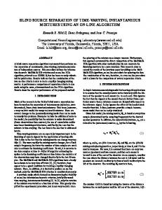
4. IMPLEMENTATION AND SIMULATION To understand the proposed decomposition method discussed in previous section. Three sources have been taken; One recording of flute of duration 4 second, one recording of guitar and one male voice sample of same duration. The duration of recording is taken of 4 second because the author want to tackle problem addressed in introduction related to frequency domain decomposition. Figure 3 shows original source signals where 1500 sample were taken for the sake of uniformity. To create a situation of blind mixing all three source signals are stored in a matrix one signal per column and multiplied with one randomly generated 3X3 matrix. In result of this a mixture of three signals are obtained shown in Figure 4. In this research two techniques are compared, one is complete decomposition of audio mixture and then clustering on the basis of similarity criterion and second method is convex divergence based independent component analysis.
0
-0.5
Fig 4 Mixed Signals in Blind Scenario Mixed Signals are decomposed in independent components without transforming the domain by using complete decomposition technique as discussed in Section-2. The independent components are shown in Figure 7 It is clearly evident that some of the components holds similarity and conclusion can made that, the independent components can be grouped by applying clustering algorithm based on similarity criteria. For clustering of independent components K- mean clustering technique is applied and resultant clusters are shown in figure 5. Cluster 1 contains two independent components, cluster 2 and cluster 3 contains 5 components in each. Last step is to apply reconstruction procedure, as all sources sound simultaneously then reconstruction can be applied as Yi (n) = Sj1 (n) + . . . . . . . . . . +SjL (n)
(7)
The reconstructed versions of signals are shown in figure 7. The quality of separated signals are evaluated by BSS_Eval function available GNU public licence and separated signals SIR values are 29.7 dB, 31.4 dB and 34.3 dB respectively.
50
International Journal of Computer Applications (0975 – 8887) Volume 132 – No.6, December2015 Cluster1 0.1 0.05 0 -0.05 -0.1
0
5000
10000
15000
0
5000
10000
15000
0.1 0.05 0 -0.05 -0.1
and scaled natural gradient technique is used for weight updation. The stopping criteria of this technique is inspired from central limit theorem, according to that independent sources have non-Gaussian profile and it is observed from experiments in blind sources separation techniques the estimated signals are in super-Gaussian in nature, irrespective to mixing condition and in result of that positive kurtosis value is taken as stopping criteria of algorithm. Cluster 3 0.1
cluster 2 0.5
0
0
-0.1
-0.5
0
5000
10000
15000
0.05
0.1
-0.2 0
5000
10000
15000
0.2
-0.2 0
5000
10000
15000
0
5000
10000
15000
0
5000
10000
15000
0
5000
10000
15000
0
5000
10000
15000
0.2
0
0 -0.2
0
5000
10000
15000
0.2
0.1
0
0 0
5000
10000
15000
Separated Source Signals
0
0
5000
10000
-0.1
Fig 6 Separated Signals
0.5
-0.5
15000
0.2
-0.2
-0.2
10000
0
0 -0.1
5000
0
0 -0.05
0
0.2
15000
0.5
Quality of separated signals using convex divergence based ICA technique is also evaluated in terms of Signal to interference ratio. BSS_Eval function is used for evaluation of SIR value. The SIR value of signal 1 is 29.80 dB, Signal 2 is 32.10 dB and for signal 3 it is 34.24 dB.
5. CONCLUSION 0
-0.5
0
5000
10000
15000
0
5000
10000
15000
1
0
-1
Fig 5 Clusters of mixed signals Second source separation technique is modified convex divergence ICA is applied for performance evaluation and details of algorithm and experimental details are given in ref [18]. Sources are estimated using NC-ICA algorithm in time domain without decomposition, as these techniques is intended to estimation of unmixing matrix base on unsupervised learning base neural structure. In this technique it is assumed that the mixing matrix is invertible and algorithm is based on estimation of inverse of mixing matrix, a modified convex divergence function is used for learning
A time domain complete decomposition based source separation method is proposed for blind audio source separation. Proposed method is a variation of T-ABCD method for blind source separation. The key objective of this paper is, to support the argument that, there is a big room for improvement in existing time domain decomposition algorithms for blind audio source separation techniques. In this paper modified divergence based algorithms and K-mean clustering method is incorporated in existing decomposition techniques. Results are evident that the performance and quality of separation is improved and Time domain complete decomposition and convex divergence based ICA techniques are close competitor. As both the techniques are exhibiting similar performance. The conclusion can be drawn that, the use of modified convex divergence base ICA in complete decomposition technique improves the quality of separation.
51
International Journal of Computer Applications (0975 – 8887) Volume 132 – No.6, December2015
0.1 0 -0.1 0.1 0 -0.1 1 0 -1 0.05 0 -0.05 0.1 0 -0.1 0.2 0 -0.2 0.2 0 -0.2 0.5 0 -0.5 0.2 0 -0.2 0.2 0 -0.2 0.2 0 -0.2 0.1 0 -0.1
0
5000
10000
15000
0
5000
10000
15000
0
5000
10000
15000
0
5000
10000
15000
0
5000
10000
15000
0
5000
10000
15000
0
5000
10000
15000
0
5000
10000
15000
0
5000
10000
15000
0
5000
10000
15000
0
5000
10000
15000
0
5000
10000
15000
Fig 7 the independent components of mixed signals [1] Emmanuel Vincent, Nancy Bertin, Remi Gribonval and Frederic Bimbot, “From Blind to Guided Audio Source Separation”, IEEE Signal Processing Magazine, pp. 107115, May 2014.
Fu Gen-Shen et al. “Complex Indpendent Component Analysis Using Three Type of Diversity: NonGaussianity, Nonwhiteness, and Noncircularity” IEEE Transactions on Signal Processing, Vol 63, No.3,pp.794805, Feb 2015
[2] Naik R. Ganesh, Kumar K Dinesh “An Overview of Independent Component Analysis and Its Applications”, Iformatica 35, pp.63-81,2011
[4] H. Sawada,R. Mukai, S. Araki and S. Makino, “A robust and precise method for solving the permutation problem of frequency-domain blind source separation”, IEEE
6. REFERENCES
[3]
52
International Journal of Computer Applications (0975 – 8887) Volume 132 – No.6, December2015 Transc Speech Audio Process, Vol.12, No. 5,pp.530538,Sep 2004
Electronics Engg. Vol. 2, Spl. Issue 1 (2015), pp.29-33 eISSN: 1694-2310 .
[5]
N. Mitianoudias, M. E Davies, “ Audio source separations of convolutive mixtures” IEEE Trans. Speech Audio and Language processing, vol. 11, no. 5, pp.489-497, Sep. 2003
[6]
E. Vincent , R. Gribonval and M. D Plomby, “Oracle estimation for benchmarking of source separation algorithms‟” Signal Processing , vol.87, no.8, pp. 19331950, Nov, 2007.
[17] N. Dubey, R.Mehra, „Comparative Analysis of Time Domain and Frequency Domain Blind Audio Source Separation Techniques”,Int. Journal of Advance Technology in engineering and sciences, Vol.3 No. 01, pp.570-577, 2015
[7]
Zbynek Koldovsky, Petr Tichavsky, “Time- Domain Blind separation of Audio Sources on the basis of a Complete ICA Decomposition of an observation space,” IEEE Trans. On Audio, Speech and Language Pross. Vol.19, no. 2, pp/ 406-416 , 2011
[8] S. C Douglas, H. Sawada and S. Makino, “Natural gradient multichannel blind deconvolution and equalization using natural gradient,” in processing IEEE workshop signal processing Adv. In wireless communication, paris, France, Apr. 1997 pp 101-104 [9]
H. Bousbia-Salah, A. Belouchrani , and K abedMeriam, “Jaccobi-like algorithm for blind signal separation of convolutive mixtures”, IEE Electronics Letter, vol. 37, no. 16, pp. 1049-1050, Aug. 2001
[10] H. Buchner, R. Aichiner and W. Kellermann,”A generalization of blind source separation algorithms for convolutive mixtures based on second-order statistics,” IEEE Transac. Speech Audio Processing, vol.13, no.1, pp. 120-134, Jan 2005. [11] C. Fevotte, A. Debiolles and C. Doncarli, “Blind separation of FIR convolutive mixtures: Applications to speech signals,” in proceedings of 1st ISCA Work hop Non-linear speech processing, 2003 [12] P. Tichavsky and A. Yeredor, “Fast approximate joint diagonalization incorporating weight matrices,” IEEE Trans. Signal Processing, vol.57, no. 3, pp. 878-891, March 2009. [13] Amari, “Natural gradient works efficiently in learning,” Neural Computing Vol. 10, pp. 251–276, 1998. [14] K. Abed-Meriam and A. Belouchrani, “ Algorithms for joint block diagonalization,” in proc. EUSIPCO‟04, Vienna, Austria 2004 pp. 209-212. [15] Z. Koldovsky, P.Tichavsky and E. Oja , “ Efficient variant of algorithm FastICA for independent component analysis,” IEEE Transc. Neural Networks, vol. 17, no.5, pp. 1265-1277, Sep. 2006
[18] N.Dubey, R. Mehra ,“ Unsupervised Learning Based Modified C-ICA for Audio Source Separation in Blind Scenario”, Accepted in Int. Journal of Information technology and computers sciences. ISSN :2074-9015 [19] Deepak Rasaily, R. Mehra, N. Dubey,” Divergence for Blind Audio Source Separation”, IJCTT, Vol.28 , No-1, pp. 01-04 [20] Devi, Rajesh Mehra, “FPGA implementation of High Speed pulse Shaping Filter for SDR applications,” Vol. 90, pp. 214-222, 2010.
7. AUTHOR PROFILE Naveen Dubey is currently associated with Electronics and Communication Engineering Department of RKG Institute of Technology for Women, Ghaziabad, India since 2008. He is ME-Scholar at National Institute of Technical Teachers‟ Training & Research, Chandigarh, India and received Bachelor of Technology from UP Technical University, Lucknow, India in 2008. Received best performer award in creativity and innovation from IIT-Delhi. He guided 20 UG projects and presented 2 projects in Department of Science and Technology, Government of India. He published and presented more than 10 papers in International conferences and journals. His research areas are Digital Signal Processing, Neural Networks and EM Fields. His research project includes Blind audio source separation. Dr. Rajesh Mehra: Dr. Mehra is currently associated with Electronics and Communication Engineering Department of National Institute of Technical Teachers‟ Training & Research, Chandigarh, India since 1996. He has received his Doctor of Philosophy in Engineering and Technology from Panjab University, Chandigarh, India in 2015. Dr. Mehra received his Master of Engineering from Panjab Univeristy, Chandigarh, India in 2008 and Bachelor of Technology from NIT, Jalandhar, India in 1994. Dr. Mehra has 20 years of academic and industry experience. He has more than 250 papers in his credit which are published in refereed International Journals and Conferences. Dr. Mehra has 55 ME thesis in his credit. He has also authored one book on PLC & SCADA. His research areas are Advanced Digital Signal Processing, VLSI Design, FPGA System Design, Embedded System Design, and Wireless & Mobile Communication. Dr. Mehra is member of IEEE and ISTE.
[16] N. Dubey, R. Mehra, „Blind Audio Source Separation: An unsupervised Approach“Int. Journal of Electrical &
IJCATM : www.ijcaonline.org
53