Blind Source Separation Using Temporal Predictability

LETTER

Communicated by Michael Lewicki

Blind Source Separation Using Temporal Predictability James V. Stone Psychology Department, Sheffield University, Sheffield, S10 2UR, England

A measure of temporal predictability is defined and used to separate linear mixtures of signals. Given any set of statistically independent source signals, it is conjectured here that a linear mixture of those signals has the following property: the temporal predictability of any signal mixture is less than (or equal to) that of any of its component source signals. It is shown that this property can be used to recover source signals from a set of linear mixtures of those signals by finding an un-mixing matrix that maximizes a measure of temporal predictability for each recovered signal. This matrix is obtained as the solution to a generalized eigenvalue problem; such problems have scaling characteristics of O(N3 ), where N is the number of signal mixtures. In contrast to independent component analysis, the temporal predictability method requires minimal assumptions regarding the probability density functions of source signals. It is demonstrated that the method can separate signal mixtures in which each mixture is a linear combination of source signals with supergaussian, subgaussian, and gaussian probability density functions and on mixtures of voices and music. 1 Introduction Almost every signal measured within a physical system is actually a mixture of statistically independent source signals. However, because source signals are usually generated by the motion of mass (e.g., a membrane), the form of physically possible source signals is underwritten by the laws that govern how masses can move over time. This suggests that the most parsimonious explanation for the complexity of a given observed signal is that it consists of a mixture of simpler source signals, each from a different physical source. Here, this observation has been used as a basis for recovering source signals from mixtures of those signals. Consider two people speaking simultaneously, with each person a different distance from two microphones. Each microphone records a linear mixture of the two voices. The two resultant voice mixtures exemplify three universal properties of linear mixtures of statistically independent source signals: 1. Temporal predictability (conjecture)—The temporal predictability c 2001 Massachusetts Institute of Technology Neural Computation 13, 1559–1574 (2001) °

1560

James V Stone

(formally defined later) of any signal mixture is less than (or equal to) that of any of its component source signals. 2. Gaussian probability density function—The central limit theorem ensures that the extent to which the probability density function (pdf) of any mixture approximates a gaussian distribution is greater than (or equal to) any of its component source signals. 3. Statistical Independence—The degree of statistical independence between any two signal mixtures is less than (or equal to) the degree of independence between any two source signals. Property 2 forms the basis of projection pursuit (Friedman, 1987), and properties 1 and 2 are critical assumptions underlying independent component analysis (ICA) (Jutten & Hérault, 1988; Bell & Sejnowski, 1995). All three properties are generic characteristics of signal mixtures. Unlike properties 2 and 3, property 1 (temporal predictability) has received relatively little attention as a basis for source separation. However, temporal predictability has been used to augment conventional source separation methods, such as ICA.1 These conventional source separation methods are defined in terms of model pdfs and their corresponding cumulative density functions (cdfs) of source signals. Such methods are invariant with respect to temporal permutations of signals. For convenience, these methods will be referred to as cdf-based blind source separation (BSS cdf) methods. Specifically, Pearlmutter and Parra (1996) incorporate a linear predictive coding (LPC) model into Bell and Sejnowski’s ICA method. This is achieved by augmenting the conventional ICA unmixing matrix W with extra parameters, which are coefficients of a LPC model. The resulting “contextual ICA” method encourages extraction of source signals that conform to both the LPC model and the high-kurtosis pdf model implicit in ICA. Attias (2000) describes a method for augmenting independent factor analysis with a first-order hidden Markov model in order to model temporal dependences within each source signal. The methods described in both Pearlmutter and Parra (1996) and Attias (2000) are demonstrated on signals that cannot be separated by ICA alone. More recently, Hyvärinen (2000) described complexity pursuit, a method in which ICA is augmented with a measure of the time dependencies of extracted sources. 2 However, each of these three methods requires the use of iterative, gradient-ascent techniques in order to locate maxima of a nonlinear merit function. The Bussgang techniques surveyed in Bellini (1994) can be shown to equalize correlations between a signal and a time-delayed version of that 1

The method described in Bell & Sejnowski (1995). Bell and Sejnowski (1995) is used as a reference point for conventional ICA methods in this article. 2 Hyv¨ arinen’s work came to my attention while this article was under revision.

Blind Source Separation Using Temporal Predictability

1561

signal, for a specific value of delay. However, Bussgang techniques also require a nonlinear function to be chosen, which is analogous to the cdf used in ICA. As with ICA, the quality of solutions can depend critically on the form chosen for this nonlinear function (Cardoso, 1998). Wu and Principe (1999) describe a BSS cdf technique for separation of source signals with nongaussian pdfs, without prior knowledge of the pdfs of source signals. In common with ICA, the method is based on the observation that source signals tend to be nongaussian. In contrast to ICA, source signals are recovered by maximizing a quadratic measure of the difference between each extracted signal and a gaussian signal with the same standard deviation as the extracted signal. One source separation method that does not explicitly rely on the pdf of extracted signals is described in Molgedey and Schuster (1994). These authors implicitly assume that a set of source signals is uncorrelated at two different time lags: L = 0 and L = 1t. This yields a general eigenvalue problem, so that the solution matrix is unique and readily obtainable using standard eigenvalue routines. One practical drawback is the method’s sensitivity to the chosen value of 1t. For example, if one of two source signals is periodic with period θ = 1t, then the solutions to the eigenvalue problem become degenerate, so that source separation fails. In this article, a method explicitly based on a simple measure of temporal predictability is introduced. The main contribution of this article is to demonstrate that maximizing temporal predictability alone can be sufficient for separating signal sources. No formal proof is given of the temporal predictability conjecture stated in previously in this section, the main purpose being to demonstrate the utility associated with this conjecture. Although counterexamples to this informal conjecture are easy to construct, a formal definition of the conjecture is robust with respect to such counterexamples (see section 1.4). Moreover, results presented here suggest that the conjecture holds true for many physically realistic signals, such as voices and music. 1.1 Problem Definition and Temporal Predictability. Consider a set of K statistically independent source signals s = {s1 | s2 | · · · | sK }t , where the ith row in s is a signal si measured at n time points (the superscript t denotes the transpose operator). It is assumed throughout this article that source signals are statistically independent, unless stated otherwise. A set of M ≥ K linear mixtures x = {x1 | x2 | · · · | xM }t of signals in s can be formed with an M × K mixing matrix A: x = As. If the rows of A are linearly independent,3 then any source signal si can be recovered from x with a 1 × M matrix Wi : si = Wi x. The problem to be addressed here consists in finding an unmixing matrix W = {W1 | W2 | · · · | WK }t such that each row

3 This condition can be satisfied (for instance) by placing each of K speakers a different distance from each of M microphones.

1562

James V Stone

vector Wi recovers a different signal yi , where yi is a scaled version of a source signal si , for K = M signals. 1.2 A Solution Strategy. The method for recovering source signals is based on the following conjecture: the temporal predictability of a signal mixture xi is usually less than that of any of the source signals that contribute to xi . For example, the waveform obtained by adding two sine waves with different frequencies is more complex than either of the original sine waves. This observation is used to define a measure F(Wi , x) of temporal predictability, which is then used to estimate the relative predictability of a signal yi recovered by a given matrix Wi , where yi = Wi x. If source signals are more predictable than any linear mixture yi of those signals, then the value of Wi , which maximizes the predictability of an extracted signal yi , should yield a source signal (i.e., yi = csi , where c is a constant). An information-theoretic analysis of the function F proves that maximizing the temporal predictability of a signal amounts to differentially maximizing the power of Fourier components with the lowest (nonzero) frequencies (see Stone, 1996b, Stone, 1999). The function F is invariant with respect to the power of low-frequency components in signal mixtures and therefore tends to amplify differentially even very low power components, which have the lowest (nonzero) temporal frequency. 1.3 Measuring Signal Predictability. The definition of signal predictability F used here is: F(Wi , x) = log

Pn (y − yτ )2 Vi V(Wi , x) = log = log Pτn=1 τ , ˜ τ − yτ )2 U(Wi , x) Ui τ =1 (y

(1.1)

where yτ = Wi xτ is the value of the signal y at time τ , and xτ is a vector of K signal mixture values at time τ . The term Ui reflects the extent to which yτ is predicted by a short-term moving average y˜ τ of values in y. In contrast, the term Vi is a measure of the overall variability in y, as measured by the extent to which yτ is predicted by a long-term moving average yτ of values in y. The predicted values y˜ τ and yτ of yτ are both exponentially weighted sums of signal values measured up to time (τ − 1), such that recent values have a larger weighting than those in the distant past: y˜ τ = λS y˜ (τ −1) + (1 − λS ) y(τ −1) :

0 ≤ λS ≤ 1

yτ = λL y(τ −1) + (1 − λL ) y(τ −1) :

0 ≤ λL ≤ 1.

(1.2)

The half-life hL of λL is much longer (typically 100 times longer) than the corresponding half-life hS of λS . The relation between a half-life h and the parameter λ is defined as λ = 2−1/ h . Note that maximizing only Vi would result in a high variance signal with no constraints on its temporal structure. In contrast, minimizing only


1563

U would result in a DC signal. In both cases, trivial solutions would be obtained for Wi because Vi can be maximized by setting the norm of Wi to be large, and U can be minimized by setting Wi = 0. In contrast, the ratio Vi /Ui can be maximized only if two constraints are both satisfied: (1) y has a nonzero range (i.e., high variance) and (2) the values in y change slowly over time. Note also that the value of F is independent of the norm of Wi , so that only changes in the direction of Wi affect the value of F4 . 1.4 Redefining Signal Predictability. One counterexample to the temporal predictability conjecture is as follows. Consider two sine wave source signals s1 and s2 with the same period such that s2 = s1 + π . The signal mixture s = s1 + s2 is zero at all time points and is therefore quite predictable. While s is intuitively predictable, the operational definition of predictability F used here is robust with respect to such counterexamples. Specifically, the value of the function F is undefined for s because if s = 0 everywhere, then Vi = Ui = 0 and F = log 0/0. Conversely, if the frequencies of s1 and s2 are not exactly the same, then the value of F is no longer undefined. The informal temporal predictability conjecture can now be restated formally in terms of the function F, as follows: if the value of F associated with a signal mixture xi is not undefined, then the value of F of each mixture is greater than (or equal to) the value of F of each source signal in that mixture. 2 Extracting Signals by Maximizing Signal Predictability 2.1 Extracting a Single Signal. Consider a scalar signal mixture yi formed by the application of a 1 × M matrix Wi to a set of K = M signals x. Given that yi = Wi x, equation (1.1) can be rewritten as F = log

Wi CWit , ˜ t Wi CW

(2.1)

i

where C is an M × M matrix of long-term covariances between signal mixtures and C˜ is a corresponding matrix of short-term covariances. The longterm covariance Cij and the short-term covariance C˜ ij between the ith and jth mixtures are defined as C˜ ij = Cij =

n X τ n X τ

(xiτ − x˜ iτ )(xjτ − x˜jτ ) (xiτ − xiτ )(xjτ − xjτ ).

(2.2)

4 Previous experience with iterative gradient ascent on F shows that the length of W i varies only a little throughout the optimization process. However, the method of solution used in this article avoids this issue.

1564

James V Stone

Note that C˜ and C need to be computed only once for a given set of signal mixtures and that the terms (xiτ − xiτ ) and (xiτ − x˜ iτ ) can be precomputed using fast convolution operations, as described in Eglen, Bray, and Stone (1997). Gradient ascent on F with respect to Wi could be used to maximize F, thereby maximizing the predictability of yi . The derivative of F with respect to Wi is ∇Wi F =

2Wi 2Wi ˜ C− C. Vi Ui

(2.3)

One optimization procedure (not used here) would consist of iteratively updating Wi until a maximum of F is located: Wi = Wi + η∇Wi F, where η is a small constant (typically, η = 0.001). Note that the function F is a ratio of quadratic forms. Therefore, F has exactly one global maximum and exactly one global minimum, with all other critical points being saddle points (Borga, 1998). This implies that gradient ascent is guaranteed to find the global maximum in F. Unfortunately, repeated application of the above procedure to a single set of mixtures extracts the same (most predictable) source signal. While this can be prevented by using procedures such as Gram-Schmidt orthonormalization, a more elegant method for extracting all of the sources simultaneously exists, as described next. 2.2 Simultaneous Source Separation. The gradient of F is zero at a solution where, from equation (2.3), Wi C =

Vi ˜ Wi C. Ui

(2.4)

Extrema in F correspond to values of Wi that satisfy equation (2.4), which has the form of a generalized eigenproblem (Borga, 1998). Solutions for Wi can therefore be obtained as eigenvectors of the matrix (C˜ −1 C), with corresponding eigenvalues γi = Vi /Ui . As noted above, the first such eigenvector defines a maximum in F, and each of the remaining eigenvectors defines saddle points in F. Note that eigenproblems have scaling characteristics of O(N3 ), where N is the number of signal mixtures. The matrix W can be obtained using a generalized eigenvalue routine. Results presented in this article were ob˜ All K signals tained using the Matlab eigenvalue function W = eig(C, C). can then be recovered: y = Wx, where each row of y corresponds to exactly one extracted signal yi . 2.2.1 Separating Mixtures for M > K. If the number M of mixtures is greater than the number K of sources signals, then a standard procedure


1565

for reducing M consists of using principal component analysis (PCA). PCA is used to reduce the dimensionality of the signal mixtures by discarding eigenvectors of x that have eigenvalues close to zero. However, in this article, only mixtures for which K = M are analyzed. 2.3 A Physical Interpretation. The solutions found by the method are the eigenvectors (W1 , W2 , . . . , WM ) of the matrix (C˜ −1 C). These eigenvectors ˜ are orthogonal in the metrics C and C: ˜ t=0 Wi CW j Wi CWjt = 0,

(2.5)

where, ˜ t= Wi CW j Wi CWjt

X (yiτ − y˜ iτ )(yjτ − y˜jτ ) τ

X = (yiτ − yiτ )(yjτ − yjτ ).

(2.6)

τ

Given equations (2.5), a simple and physically realistic interpretation of the method can be demonstrated. Consider the short-term and long-term half-life parameters hS and hL in the limits (hS → 0) and (hL → ∞). First, in the limit (hS → 0), the short-term mean is y˜ τ ≈ yτ −1 , and therefore (yτ − y˜ τ ) ≈ dyτ /dτ = y0τ . Second, if y has zero mean, then in the limit (hL → ∞), the long-term mean y ≈ 0, and therefore (yτ − yτ ) ≈ yτ . In these limiting cases, equations (2.5) and (2.6) imply that E[y0i yj0 ] = 0 E[yi yj ] = 0,

(2.7)

where E[ ] denotes an expectation value. Thus, one interpretation of the method is that each signal yi = Wi x is uncorrelated with every other signal yj = Wj x, and the temporal derivative y0i = Wi x0 of each extracted signal is uncorrelated with the temporal derivative yj0 = Wj x0 of every other extracted signal, where x0 is a vector variable that is the temporal derivative of the mixtures x. Critically, if two signals yi and yj are statistically independent then the conditions specified in equation (2.7) are met. Therefore, mixtures of independent signals are guaranteed to be separable by the method, at least in the limiting cases specified above. 3 Results Three experiments using the method described above were implemented in Matlab. In each experiment, K source signals were used to generate M =

1566

James V Stone

Table 1: Correlation Magnitudes Between Source Signals and Signals Recovered from Mixtures of Source Signals with Different pdfs. Source Signals

Signals Recovered

s1

s2

s3

y1 y2 y3

0.000 1.000 0.042

0.001 0.000 0.999

1.000 0.000 0.002

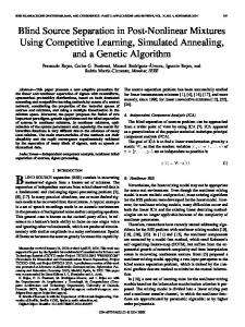
K signal mixtures, using a K × K mixing matrix, and these M mixtures were used as input to the method. Each mixture signal was normalized to have zero-mean and unit variance. Each mixing matrix was obtained using the Matlab randn function. The short-term and long-term half-lives defined in equation (1.2) were set to hS = 1 and hL = 9000, respectively. Correlations between source signals and recovered signals are reported as absolute values. Results were obtained in under 60 seconds on a Macintosh G3 (233 MHz) for all experiments reported here, using nonoptimized Matlab code. In each case, an un-mixing matrix was obtained as the solution to a generalised eigenvalue problem using the Matlab eigenvalue function ˜ W = eig(C, C). 3.1 Separating Mixtures of Signals with Different Pdfs. Three source signals s = {s1 | s2 | s3 }t are displayed in Figure 2: (1) a supergaussian signal (the sound of a gong), (2) a subgaussian signal (a sine wave), and (3) a gaussian signal. Signal 3 was generated using the randn procedure in Matlab, and temporal structure was imposed on the signal by sorting its values in ascending order. These three signals were mixed using a random matrix A to yield a set of three signal mixtures: x = As. Each signal consisted of 3000 samples; the first 1000 samples of each mixture are shown in Figure 1. The correlations between source signals and recovered signals are given in Table 1. The three recovered signals each had a correlation of r > 0.99, with only one of the source signals, and other correlations were close to zero. Note that the mixtures used here do not include any temporal delays or echoes. 3.2 Separating Mixtures of Sounds. For each experiment reported here, 50,000 data points were sampled at a rate 44,100 Hz, using a microphone to record different voices from a VHF radio onto a Macintosh computer. Two sets of eight sounds were recorded: male and female voices and classical music, with and without singing. 3.2.1 Separating Voices. The method was tested on mixtures of normal speech. Correlations between each source signal and every recovered signal for four and eight voices are given in Tables 2 and 3, respectively. Graphs


1567

Figure 1: Three signal mixtures used as input to the method. See Figure 2 for a description of the three source signals used to synthesize these mixtures. Only the first 1000 of the 9000 samples used in experiments are shown here. The ordinal axis displays signal amplitude.

of original (source) voice amplitudes and the signals recovered from a set of four mixtures (not shown) are shown in Figure 3. Note that correlations are approximately r = 0.99. With correlations this high, it is not possible to hear the difference between the original and recovered speech signals. A correlation of 0.956 was found between source 8 and recovered signal 3; this represents the worst performance of the method out of all data sets described in this article. Table 2: Correlation Magnitudes Between Each of Four Source Signals and Every Signal Recovered (y1 , . . . , y4 ) by the Method. Source Signals (voices)

Signal Recovered

s1

s2

s3

s4

y1 y2 y3 y4

0.097 0.996 0.002 0.030

0.994 0.081 0.042 0.076

0.028 0.012 0.995 0.101

0.049 0.019 0.095 0.992

Note: Each source signal has a high correlation with only one recovered signal.

1568

James V Stone

Figure 2: Three signals with different probability density functions. A supergaussian gong sound, a subgaussian sine wave, and sorted gaussian noise (see text) are displayed from top to bottom respectively. In each graph, the source signals used to synthesize the mixtures displayed in Figure 1 are shown as a solid line, and corresponding signals recovered from those mixtures are shown as dotted lines. Each source signal and its corresponding recovered signal have been shifted vertically for display purposes. The correlations between source and recovered signals are greater than r = 0.999 (see Table 1). Only the first 1000 of the 9000 samples used are shown here. The ordinal axis displays signal amplitude.

3.2.2 Separating Music. The method was tested on mixtures of eight segments of music. Correlations between each source signal and each recovered signal for eight music segments are given in Table 4. Again, correlations are approximately r = 0.99, and it is not possible to hear the difference between the original and recovered music signals. The method seems to be largely insensitive to the values used for the short-term and long-term half-lives defined in equation 1.2, provided the latter is much larger than the former. 3.3 How Maximizing Predictability Can Fail. The method is based on the assumption that different source signals are associated (via Wi ) with distinct critical points in F. However, if any two source signals have the


1569

Figure 3: Four voices (two male and two female). In each graph, the source signals used to synthesize four mixtures (not shown) are shown as solid lines, and corresponding signals recovered from these mixtures are in shown as dotted lines. Each source signal and its corresponding recovered signal have been shifted vertically for display purposes. The correlations between source and recovered signals are greater than r = 0.99 (see Table 2). Only the first 1000 of the 50,000 samples used are shown here. The ordinal axis displays signal amplitude. Table 3: Correlation Magnitudes Between Each of Eight Source Signals and Every Signal Recovered by the Method. Source Signals (voices)

Signal Recovered

s1

s2

s3

s4

s5

s6

s7

s8

y1 y2 y3 y4 y5 y6 y7 y8

0.001 0.994 0.179 0.015 0.004 0.010 0.027 0.015

0.008 0.013 0.001 0.012 0.020 0.003 0.999 0.003

0.004 0.003 0.162 0.007 0.993 0.026 0.012 0.027

0.003 0.001 0.011 0.999 0.000 0.018 0.002 0.022

0.028 0.001 0.037 0.024 0.021 0.021 0.000 0.998

0.046 0.017 0.102 0.032 0.008 0.992 0.010 0.020

0.988 0.016 0.134 0.004 0.007 0.044 0.009 0.021

0.143 0.109 0.956 0.004 0.109 0.111 0.002 0.043


1570

James V Stone

Table 4: Correlation Magnitudes Between Each of Eight Source Signals and Every Signal Recovered (y1 , . . . y8 ) by the Method. Source Signals (classical music)

Signal Recovered

s1

s2

s3

s4

s5

s6

s7

s8

y1 y2 y3 y4 y5 y6 y7 y8

0.096 0.088 0.006 0.028 0.005 0.995 0.000 0.008

0.993 0.032 0.070 0.044 0.007 0.083 0.001 0.027

0.001 0.000 0.005 0.018 0.998 0.001 0.075 0.022

0.001 0.002 0.001 0.002 0.066 0.008 0.997 0.012

0.019 0.000 0.016 0.068 0.006 0.007 0.002 0.995

0.030 0.991 0.094 0.034 0.009 0.055 0.002 0.006

0.035 0.038 0.085 0.991 0.021 0.018 0.000 0.098

0.043 0.086 0.990 0.093 0.010 0.007 0.000 0.019


same degree of predictability F, then two eigenvectors Wi and Wj have equal eigenvalues (and are associated with the same critical points in F). Therefore, any vector Wk that lies in the plane defined by Wi and Wj also maximizes F, but Wk cannot (in general) be used to extract a source signal. This has been demonstrated (not shown here) by creating two mixtures x = As from two signals s1 and s2 , where s1 is a time-reversed version of s2 . Although s1 and s2 have different time courses, they share exactly the same degree of predictability F and cannot be extracted from the mixtures x using this method. In practice, signals from different sources (e.g., voices) typically can be separated because each source signal has a unique degree of predictability (i.e., value of F). Indeed, every set of signals in which each signal is from a physically distinct source (e.g., voices) has been successfully separated in the many experiments used in the preparation of this article. 4 Discussion Methods for recovering statistically independent source signals from signal mixtures work by taking advantage of generic differences between the properties of signals and their mixtures. Three such differences were summarized in the introduction: (1) temporal predictability (conjecture) (the temporal predictability of any signal mixture is less than (or equal to) that of any of its component source signals), (2) gaussian probability density function (the central limit theorem ensures that the extent to which the pdf of any mixture approximates a gaussian distribution is greater than or equal to any of its component source signals), and (3) statistical independence (the degree of statistical independence between any two signal mixtures is less than or equal to the degree of independence between any two source sig-


1571

nals). The last two have previously been used as a basis for signal separation, and the first has been used to augment source separation (e.g., Pearlmutter & Parra, 1996; Attias, 2000; Porrill, Stone, Berwick, Mayhew, & Coffey, 2000). In this article, only the first property (temporal predictability) has been used to separate signal mixtures. While the method has a low-order polynomial time complexity of O(N3 ), this does not necessarily imply that it finds solutions more quickly than other source separation methods (see Comon & Chevalier, 2000, for an analysis of the time complexity of ICA methods). However, the fact that each simulation reported here was run in under 60 seconds (on a Macintosh G3) may indicate that the method is reasonably fast. This issue can be resolved only by a direct comparison of different methods on the same data sets. One desirable property of method described in this article is that local extrema are not an issue. This contrasts with other methods for which the existence of local extrema may be difficult to detect (Ding, Hohnson, & Kennedy, 1994). Of the methods reviewed in section 1, the method that Molgedey and Schuster (1994) described is mathematically most similar to the one described in this article, inasmuch as both methods involve a generalized eigenvalue problem. As stated in section 1, Molgedey and Schuster implicitly assume that source signals are uncorrelated at two different time lags. In contrast, one interpretation of the assumptions underlying the method presented here is that source signals are uncorrelated and their corresponding temporal derivatives are also uncorrelated (in the limiting cases specified in ection 2.3). Thus, although both methods can be formulated as generalized eigenvalue problems, the assumptions required by each method regarding the nature of source signals are qualitatively very different. As defined above, the predictions (yτ and y˜ τ ) of each signal value yτ are based on a linear weighted sum of previous values {y}. Natural extensions to this method could involve defining predicted values of yτ as general functions of previous signal values {y}, yielding functionals of the general form Pn ( f ({y} − yτ )2 . (4.1) G = log Pτn=1 2 τ =1 (g({y} − yτ ) Here, the functions f and g provide predictions of yτ , based on previous values {y} of yi , such that G is invariant with respect to the norm of Wi (recall that y = Wi x). For example, the functions f and g could be defined in terms of linear predictive coefficients, as in Pearlmutter and Parra (1996), or in terms of the exponents p and q in f (y) = yp , g(y) = yq . The ability to incorporate specific types of models into the method could also be used to deal with signal sources that contain echoes and delays. More generally, information-theoretic measures of temporal structure, such as approximate entropy (Pincus & Singer, 1996), may prove useful as measures of temporal predictability for source separation (approximate entropy was investigated

1572

James V Stone

in the development of the method presented here). In particular, the issue of sensor (e.g., microphone) noise has not been addressed in this article, and these more elaborate measures of predictability may be robust with respect to such noise. It is noteworthy that the principles underlying the method have been used for unsupervised learning in artificial neural networks (Stone, 1996a, 1996b, 1999; Becker & Hinton, 1992; Becker, 1993). This principle is useful for both unsupervised learning and source signal separation precisely because it is based on a fundamental property of the physical world: temporal predictability. However, predictability is not only a property of the temporal domain; an obvious extension (explored in Becker & Hinton, 1992; Eglen et al., 1997; Stone & Bray, 1995) is to apply the principle to the spatial domain. Additionally, the assumptions of temporal or spatial predictability used in the methods just described can be combined in a method that assumes a degree of temporal and spatial predictability. Specifically, methods that maximize predictability in space or predictability in time can be replaced by a method that maximizes predictability over space and time. An analogous spatiotemporal ICA method has been described in Stone, Porrill, Buchel, and Friston (1999). If all three properties listed above apply to any statistically independent source signals and their mixtures, a method that relies on constraints from all of these properties might be expected to deal with a wide range of signal types. It is widely acknowledged that ICA forces statistical independence on recovered signals, even if the underlying source signals are not independent. Similarly, the current method may impose temporal predictability on recovered signals even where none exists in the underlying source signals. Therefore, a method that incorporates constraints from all three properties should be relatively insensitive to violations of the assumptions on which the method is based. A framework for incorporating experimentally relevant constraints based on physically realistic properties has been formulated in the form of weak models (Porrill et al., 2000) and has been used to constrain ICA’s solutions. In particular, the function F has the correct form for a weak model and has been shown to improve solutions found by ICA (Stone & Porrill, 1999). Finally, the method described here may be useful in the analysis of medical images and electroencephalogram data. In a seminal article, Bell and Sejnowski (1995) compared their ICA method to Becker and Hinton’s IMAX method (1992) and speculated that “some way may be found to view the two in the same light.” In fact, if the hidden layers of nonlinear units in a temporal IMAX network (Becker, 1992) are removed, then the resultant system of equations is given by equation 1.1 in the limits (hS → 0) and (hL → ∞). The two methods can then be viewed in the same light: whereas ICA recovers source signals by maximizing the mutual information between input and output, (temporal) IMAX and the method described here recover source signals by maximizing the mutual information I(yτ ; yτ −1 ) between a recovered signal y at time τ and time (τ − 1).


1573

Acknowledgments Thanks to J. Porrill for discussions of the generalized eigenvalue method. Thanks to R. Lister, D. Johnston, N. Hunkin, S. Isard, K. Friston, D. Buckley, and two anonymous referees for comments on this article. This research was supported by a Mathematical Biology Wellcome Fellowship (Grant Number 044823). References Attias, H. (2000). Independent factor analysis with temporally structured factors. In S. A. Solla, T. K. Leen, & K.-R. M. (Eds.), Advances in neural information processing systems, 12. Cambridge, MA: MIT Press. Becker, S. (1993). Learning to categorize objects using temporal coherence. In S. J. Hanson, J. Cowan, & C. L. Giles (Eds.), Neural information processing systems, 5 (pp. 361–368). San Mateo, CA: Morgan Kaufmann. Becker, S., & Hinton, G. (1992). Self-organizing neural network that discovers surfaces in random-dot stereograms. Nature, 335, 161–163. Bell, A., & Sejnowski, T. (1995). An information-maximization approach to blind separation and blind deconvolution. Neural Computation, 7, 1129–1159. Bellini, S. (1994). Bussgang techniques for blind deconvolution and equalization. In S. Haykin (Ed.), Blind deconvolution (pp. 8–59). Englewood Cliffs, NJ: Prentice Hall. Borga, M. (1998). Learning multidimensional signal processing. Unpublished doctoral dissertation Linkoping University, Linkoping, Sweden. Cardoso, J. (1998). On the stability of some source separation algorithms. In Proceddings of Neural Networks for Signal Processing ’98 (pp. 13–22). Cambridge, England. Comon, P., & Chevalier, P. (2000). Blind source separation: Models, concepts, algorithms and performance. In S. Haykin (Ed.), Unsupervised adaptive filtering, Vol. 1: Blind source separation (pp. 191–235). New York: Wiley. Ding, Z., Hohnson, C., & Kennedy, R. (1994). Global convergence issues with linear blind adaptive equalizers. In S. Haykin (Ed.), Blind deconvolution (pp. 60– 115). Englewood Cliffs, NJ: Prentice Hall. Eglen, S., Bray, A., & Stone, J. (1997). Unsupervised discovery of invariances. Network, 8, 441–452. Friedman, J. (1987). Exploratory projection pursuit. Journal of the American Statistical Association, 82(397), 249–266. Hyvärinen, A. (2000). Complexity pursuit: Combining nongaussinity and autocorrelations of signal separation. In Proc. Int. Workshop on Independent Component Analysis and Blind Signal Separation (ICA2000) (pp. 175–180). Helsinki, Finland. Jutten, C., & Hérault, J. (1988). Independent component analysis versus pca. In Proc. EUSIPCO (pp. 643–646). Molgedey, L., & Schuster, H. (1994). Separation of a mixture of independent signals using time delayed correlations. Physical Review Letters, 72(23), 3634– 3637.

1574

James V Stone

Pearlmutter, B., & Parra, L. (1996). A context-sensitive generalization of ica. In International Conference on Neural Information Processing. Hong Kong. Available online at: http://www.cs.unm.edu/∼bap/publications.html#journal. Pincus, S., & Singer, B. (1996). Randomness and degrees of irregularity. Proceedings of the National Academy of Sciences USA, 93, 2083–2088. Porrill, J., Stone, J. V, Berwick, J., Mayhew, J., & Coffey, P. (2000). Analysis of optical imaging data using weak models and ICA. In M. Girolami (Ed.), Advances in independent component analysis. Berlin: Springer-Verlag. Stone, J. V (1996a). A canonical microfunction for learning perceptual invariances. Perception, 25(2), 207–220. Stone, J. V (1996b). Learning perceptually salient visual parameters through spatiotemporal smoothness constraints. Neural Computation, 8(7), 1463–1492. Stone, J. V (1999). Learning perceptually salient visual parameters using spatiotemporal smoothness constraints. In G. Hinton & T. Sejnowski (Eds.), Unsupervised learning: Foundations of neural computation (pp. 71–100). Cambridge, MA: MIT Press. Stone, J. V, & Bray, A. (1995). A learning rule for extracting spatio-temporal invariances. Network, 6(3),1–8. Stone, J. V, & Porrill, J. (1999). Regularisation using spatiotemporal independence and predictability (Tech. Rep. No. 201). Sheffield: Sheffield University. Stone, J. V, Porrill, J., Buchel, C., & Friston, K. (1999). Spatial, temporal, and spatiotemporal independent component analysis of FMRI data. In K. V. Mardia, R. G. Aykroyd, & I. L. Dryden (Eds.), Proceedings of the 18th Leeds Statistical Research Workshop on Spatial-Temporal Modelling and Its Applications (pp. 23–28). Leeds: Leeds University Press. Wu, H., & Principe, J. (1999). A gaussianity measure for blind source separation insensitive to the sign of kurtosis. In Neural Networks for Signal Processing IX: Proceedings of the 1999 Signal Processing Society Workshop (pp. 58–66). Received February 24, 2000; accepted September 8, 2000.