Blur Identification Using Neural Network for Image Restoration

Preprint. Proceedings 9th Fuzzy Days Conference Dortmund, September 2006

Blur Identification Using Neural Network for Image Restoration Igor Aizenberg1, Dmitriy Paliy2, Claudio Moraga3,4 and Jaakko Astola2 1Texas

A&M University-Texarkana, P.O. Box 5518, 2600 N. Robison Rd. Texarkana, Texas 75505 USA; [email protected] 2Tampere University of Technology, Institute for Signal Processing TICSP, Tampere University of Technology P.O. Box 553 FIN-33101 Tampere Finland [email protected] 3 European Centre for Soft Computing. 33600 Mieres, Asturias, Spain 4University of Dortmund, Department of Computer Science 1,

44221 Dortmund, Germany, [email protected]

Abstract. A prior knowledge about the distorting operator and its parameters is of crucial importance in blurred image restoration. In this paper the continuousvalued multilayer neural network based on multi-valued neurons (MLMVN) is exploited for identification of a type of blur among six trained blurs and of its parameters. This network has a number of specific properties and advantages. Its backpropagation learning algorithm does not require differentiability of the activation function. The functionality of the MLMVN is higher than the ones of the traditional feedforward neural networks and a variety of kernel-based networks. Its higher flexibility and faster adaptation to the mapping implemented make possible an accomplishment of complex problems using a simpler network. Therefore, the MLMVN can be used to solve those nonstandard recognition and classification problems that cannot be solved using other techniques.

1

Introduction

A multilayer neural network based on multi-valued neurons (MLMVN) has been introduced in [1] and then investigated and developed further in [2]. This network consists of multi-valued neurons (MVN). That is a neuron with complex-valued weights and an activation function, defined as a function of the argument of a weighted sum. This activation function was proposed in 1971 in the pioneer paper of N. Aizenberg et al. [3]. The multi-valued neuron was introduced in [4]. It is based on the principles of multiple-valued threshold logic over the field of complex numbers formulated in [5] and then developed in [6]. A comprehensive observation of the discrete-valued MVN, its properties and learning is presented in [6]. A continuous-valued MVN and its learning are considered in [1],[2]. In this paper we consider the continuous-valued

MVN (further simply MVN) only. The most important properties of MVN are: the complex-valued weights, inputs and output lying on the unit circle, and the activation function, which maps the complex plane into the unit circle. It is important that MVN learning is reduced to the movement along the unit circle. The MVN learning algorithm is based on a simple linear error correction rule and it does not require differentiability of the activation function. Different applications of MVN have been considered during recent years, e.g.: MVN as a basic neuron in the cellular neural networks [6], as the basic neuron of the neural-based associative memories [6],[7]-[10], as the basic neuron in a variety of pattern recognition systems [10]-[12], and as a basic neuron of the MLMVN [1],[2]. The MLMVN outperforms a classical multilayer feedforward network and different kernel-based networks in the terms of learning speed, network complexity, and classification/prediction rate tested for such popular benchmarks problems as the parity n, the two spirals, the sonar, and the Mackey-Glass time series prediction [1],[2]. These properties of MLMVN show that it is more flexible and adapts faster in comparison with other solutions. In this paper we apply MLMVN to identify blur and its parameters, which is a key problem in image restoration. Usually blur refers to the low-pass distortions introduced into an image. It can be caused, e.g., by the relative motion between the camera and the original scene, by the optical system which is out of focus, by atmospheric turbulence (optical satellite imaging), aberrations in the optical system, etc. [13]. Any type of blur, which is spatially invariant, can be expressed by the convolution kernel in the integral equation [14],[15]. Hence, deblurring (restoration) of a blurred image is an ill-posed inverse problem [16], and regularization is commonly used when solving this problem [16]. There is a variety of sophisticated and efficient deblurring techniques such as deconvolution based on the Wiener filter [13],[17], nonparametric image deblurring using local polynomial approximation with spatially-adaptive scale selection based on the intersection of confidence intervals rule [17], Fourier-wavelet regularized deconvolution [18], expectation-maximization algorithm for wavelet-based image deconvolution [19], etc. All these techniques assume a prior knowledge of the blurring kernel or its point spread function (PSF) and its parameter. When the blurring operator is unknown, the image restoration becomes a blind deconvolution problem [20]-[22]. Most of the methods to solve it are iterative, and, therefore, they are computationally costly. Due to the presence of noise they suffer from the stability and convergence problems [23]. The original solutions of blur identification problem that are based on the use of MVN-based neural networks were proposed in [12], [24] and [25]. Two different single-layer MVN-based networks have been used to identify blur and its parameter (e.g., variation for the Gaussian blur, extent for motion blur, etc.) in [24]. The results were good, but this approach had some disadvantages. For instance, the networks used have specific architecture with no universal learning algorithm, thus each neuron was trained separately. Another disadvantage is the use of too many spectral coefficients as features (quarter of image size). Thus the learning process was heavy. Significant improvement was obtained in [25] comparing to [24]. A single neural

network (the discrete-valued MLMVN) with the original backpropagation training scheme was used to identify both smoothing operator and its parameter on a single observed noisy image. However, the discrete-valued MLMVN in [25] had such a drawback as discrete inputs which results in quantization error of pattern vectors. This reduces its applicability. In this paper, we propose to use the continuous-valued MLMVN (further simply MLMVN) to solve both the blur and its parameters identification problems in order to overcome the disadvantages mentioned above. The modification of the MLMVN results in significant improvement of the functionality.

2

Image Restoration Problem

Mathematically, a variety of image capturing principles can be modelled by the 2 Fredholm integral of the first kind in space z (t ) = ∫ v (t , l ) y (l )dl , where X

t, l ∈ X ⊂

2

, v is a point-spread function (PSF) of a system, y is an image

intensity function, and z (t ) is an observed image [15]. A natural simplification is that the PSF v is shift-invariant which leads to a convolution operation in the observation model. We assume that the convolution is discrete and noise is present. Hence, the observed image z given in the following form: z (t ) = (v ⊗ y )(t ) + ε (t ), (1) where " ⊗ " denotes the convolution, t is defined on the regular L1 × L2 lattice, t ∈ X = {(t1 , t2 ); ti = 0,1,..., Li − 1, i = 1, 2} , and ε (t ) is a noise. It is assumed that the

noise is white Gaussian with zero-mean and variance σ 2 , ε (t ) ~ N (0, σ 2 ) . In the 2D frequency domain the model (1) takes the form: Z (ω ) = V (ω )Y (ω ) + ε (ω ), (2) ⋅ where Z (ω ) = F{z (t )} is a representation of a signal z in a Fourier domain and F{} is a discrete Fourier transform, V (ω ) = F {v(t )}, Y (ω ) = F { y (t )}, ε (ω ) = F {ε (t )} ,

and

ω ∈W ,

W = {(ω1 , ω2 ); ωi = 2π ki /Li , ki = 0,1,..., Li − 1,

i = 1, 2}

is

the

normalized 2D frequency. The removal of the degradation caused by a PSF is an inverse problem, widely referred as a deconvolution. Usually this problem is ill-posed which results in the instability of a solution, i.e. it is highly sensitive to the noise. The stability can be provided by constraints imposed on the solution. A general approach to this kind of problems refers to the methods of Lagrange multipliers and the Tikhonov regularization [16]. The regularized inverse filter can be obtained as a solution of the least square problem with a penalty term:

J = Z − VY 2 + α Y 2, 2

2

where α ≥ 0 is a regularization parameter and ⋅

(3) denotes l − norm. Here, the first 2

2

term Z − VY

2 2

gives the fidelity to the available data Z and the second term bounds

the power of this estimate by means of the regularization parameter α . In (3), and further, we omit the argument ω in the Fourier transform variables. We obtain the solution in the following form by minimizing (3):

Y=

V V +α 2

Z , $yα ( x) = F −1{Y } .

(4)

where Y is an estimate of Y , and V denotes complex-conjugate value of V . In this paper we consider Gaussian, motion, rectangular (boxcar) and diagonal blurs. We aim to identify both blur, which is characterized by PSF, and its parameter using a single network. The PSF v describes how the point source of light is spread over the image plane. It is one of the main characteristics of the optical system. For a variety of devices, like photo or video camera, microscope, telescope, etc., PSFs are often approximated by the Gaussian function: ⎛ t12 + t22 ⎞ 1 v(t ) = exp − 2 ⎟ (5) ⎜ 2πτ 2 τ ⎠ ⎝ where τ 2 is a parameter of the PSF (the variance of the Gaussian function) (Fig. 2a). Its Fourier transform V is also a Gaussian function and its absolute values | V | are shown in Fig. 2d. Another example of blur is a uniform linear motion which happens while taking a picture of a moving object relatively to the camera: ⎧1 ⎪ , t12 + t22 < h / 2, t1 cos φ = t2 sin φ , v(t ) = ⎨ h (6) otherwise, ⎪⎩ 0, where h is a parameter which depends on the velocity of the moving object and describes the length of motion in pixels, and φ is the angle between the motion orientation and the horizontal axis. Any uniform function like (6) is characterized by the number of slopes in the frequency domain (Fig. 2b,e). The uniform rectangular blur is described by the following function (Fig. 2c): h h ⎧1 ⎪ , t < , t < , v(t ) = ⎨ h 2 1 2 2 2 (7) ⎪⎩ 0, otherwise,

where parameter h defines the size of smoothing area. The frequency characteristics of (7) are shown in Fig. 2f. In order to solve equation (4) one should know PSF V . In this paper we propose to use a neural network to recognize type and parameter of V from the noisy observation Z .

3

Multilayer Neural Network Based On Multi-Valued Neurons

A continuous-valued MVN has been introduced in [1],[2]. It performs a mapping between n inputs and a single output using n+1 complex-valued weights f ( x1 , ..., xn ) = P ( w0 + w1 x1 + ... + wn xn ) , (8) where X = ( x1 ,...,xn ) is a vector of complex-valued inputs (a pattern vector) and

W = ( w0 ,w1 , ...,wn ) is a weighting vector. P is the activation function of the neuron: P( z ) = exp(i (arg z )) = eiArg z =

z , |z|

(9)

where z = w0 + w1 x1 + ... + wn xn is a weighted sum, arg z is an argument of the complex number z, Arg z is a main value of the argument of the complex number z and |z| is its modulo. The function (9) maps the complex plane into a whole unit circle. The MVN learning is reduced to the movement along the unit circle. This movement does not require differentiability of the activation function. Any direction along the circle always leads to the target. The shortest way of this movement is completely determined by an error that is a difference between the desired and actual outputs. The corresponding learning rule is [1],[2]: Wr+1 = Wr +

Cr Cr ⎛ q z ⎞ (ε q - eiArg z ) X = Wr + ⎜ε ⎟ X. (n+1) (n+1) ⎝ | z |⎠

(10)

where X denotes vector with the complex-conjugated elements to input pattern vector X, Wr is a current weighting vector, Wr +1 is a weighting vector after correction, Cr is a learning rate. A modified learning rule is [1],[2]:

Cr ⎛ q z ⎞ (11) ⎜ε ⎟X , (n+1) zr ⎝ | z |⎠ where zr is a current value of the weighted sum. A multilayer feedforward neural network based on multi-valued neurons (MLMVN) has been proposed in [1],[2]. It refers to the basic principles of the network with a feedforward dataflow through nodes proposed in [26] by D. E. Rumelhart and J. L. McClelland. The most important is that there is a full connection between the consecutive layers (the outputs of neurons from the preceding layer are connected with the corresponding inputs of neurons from the following layer). The network contains one input layer, m-1 hidden layers and one output layer. Let us use here the following notations. Let Tkm be a desired output of the kth neuron from the Wr+1 = Wr +

mth (output) layer; Ykm be an actual output of the kth neuron from the mth (output) layer. Then the global error of the network taken from the kth neuron of the mth (output) layer is calculated as follows: * δ km = Tkm − Ykm . (12) The square error functional for the sth pattern X s = ( x1 ,...,xn ) is as follows:

* 2 Es = ∑ (δ km ) (W ) , k

(13)

where δ km is a global error taken from the kth neuron of the mth (output) layer, Es is a square error of the network for the sth pattern, and W denotes all the weighting vectors of all the neurons of the network. The mean square error functional for the network is defined as follows: *

Ε=

1 N

N

∑E s =1

s

,

(14)

where N is a total number of patterns in the training set. Following the backpropagation learning algorithm for the MLMVN proposed in [1],[2], the errors of all the neurons from the network are determined by the global errors of the network (12). Finally, the MLMVN learning is based on the minimization of the error functional (14). It is fundamental that the global error of the network consists not only of the output neurons errors, but of the local errors of the output neurons and hidden neurons. It means that in order to obtain the local errors for all neurons, the global error must be shared among these neurons. Let us use the following notations. Let wikj be the weight corresponding to the ith input of the kjth neuron (kth neuron of the jth level), Y ij be the actual output of the ith neuron from the jth layer (j=1,…,m), and N j be the number of the neurons in the jth layer (it means that the neurons from the j+1st layer have exactly N j inputs). Let x1 ,..., xn be the network inputs.

Hence, the local errors are represented in the following way. The errors of the mth (output) layer neurons are: 1 * δ km = δ km , (15) sm where km is a kth neuron of the mth layer; sm = Nm−1 + 1 , i.e. the number of all neurons on the previous layer (layer m-1 which the error is backpropagated to) incremented by 1. The errors of the hidden layers neurons are computed as follows:

1 δ kj = sj

N j +1

∑δ i =1

ij +1

( wkij +1 ) −1 ,

(16)

where kj specifies the kth neuron of the jth layer (j=1,…,m-1); s j = N j −1 + 1, j = 2,..., m, s1 = 1 is the number of all neurons on the layer j-1 incremented by 1. Thus, the equations (15),(16) determine the error backpropagation for MLMVN. It is worth to stress on its principal distinction from the classical error backpropagation: the equations (15),(16) do not contain a derivative of the activation function! A factor 1/ s j in (15),(16) ensures sharing of the particular neuron error among all the neurons on which this error depends. It should be mentioned that for the 1st hidden layer the parameter s1 = 1 because there is no previous hidden layer, and there are no neurons the error may be shared with.

The weights for all neurons of the network are corrected after calculation of the errors. In order to do that, we use the learning rule (10) (for the output layer) and (11) (for the hidden layers). Hence, the following correction rules are used for the weights [1],[2]: Ckm δ kmY%im −1 , i = 1,..., n, w% ikj = wikm + ( N m + 1) (17) Ckm δ km , w% 0km = w0km + ( N m + 1) th for the neurons from the m (output) layer (kth neuron of the mth layer), w% ikj = wikj + w% 0kj = w0kj +

Ckj ( N j + 1) | zkj | Ckj ( N j + 1) | zkj |

δ kj Y%i j −1 , i = 1,..., n, (18)

δ kj ,

for the neurons from the 2 till m-1st hidden layers (kth neuron of the jth layer (j=2, …, m-1), and Ck1 δ k1 xi , i = 1,..., n, w% ik1 = wik1 + (n + 1) | zk1 | (19) Ck1 k1 k1 % δ k1 , w0 = w0 + (n + 1) | zk1 | for the neurons of the 1st hidden layer. It should be mentioned that in our simulations we used Ckj = 1 in (17)-(19). nd

In general, the learning process should continue until the following condition is satisfied: 1 N 1 N * 2 E = ∑∑ (δ km (20) ∑ Es ≤ λ , s ) (W ) = N s =1 k N s =1 where λ determines the precision of learning. In particular, in the case when λ = 0 * the equation (20) is transformed to ∀k , ∀s δ km s = 0.

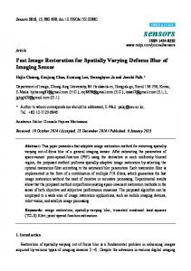
Fig. 1. Structure of the neural element on the output layer of MLMVN.

4

Simulations

4.1 Training Set Formation

The observed image z(t) is modeled as the output of a linear shift-invariant system (1) which is characterized by the PSF v. Since in the frequency domain this model is a product of the true object function Y and V we state the problem as a recognition of the shape of V and its parameters from the power-spectral density (PSD) of the observation Z, i.e. from Z = Z ⋅ Z . In terms of statistical expectation we can rewrite 2

that as follows:

{ } = E { YV + n } = Y

E Z

2

2

2

V +σ 2 2

(21)

where σ 2 is the variance of noise in (2). Examples of log Z values are shown in Fig. 3. The distortions of PSD for the test image Cameraman (Fig. 3a) that are typical for each type of blur (Fig. 3b,c) are clearly visible in Fig. 3f,g. For the sake of simplicity we consider the image z(t) with the equal sizes, i.e. L = L1 = L2 in (1),(2). In order to obtain the training vector X = ( x1 ,..., xn ) in (19) as an input data of the network, and taking into account that the PSF v is symmetrical, PSD of z(t) (21) is used as follows: ⎛ log Z ωk1 , k2 − log ( Z min ) ⎞ ⎟, x j = exp ⎜⎜ 2π i ⋅ ( K − 1) (22) − log Z log Z ( max ) ( min ) ⎟⎟ ⎜ ⎝ ⎠ where for k1 = k2 , k2 = 1,..., L / 2 − 1, ⎧ j = 1,..., L / 2 − 1, ⎪ for k1 = 1, k2 = 1,..., L / 2 − 1, (23) ⎨ j = L / 2,..., L − 2, ⎪ j = L − 1,...,3L / 2 − 3, for k = 1, k = 1,..., L / 2 − 1, 2 1 ⎩

( (

( (

and Z max = max k1 , k2 Z ωk1 , k2

)) ,

))

( (

Z min = min k1 , k2 Z ωk1 , k2

)) ,

and K is a number of

sectors in (9). Eventually, the length of the pattern vector is n= 3L / 2 − 3 . Some examples of vectors of PSD log values multiplied by K-1 used in (22),(23) to obtain the input training vector X are shown in Fig. 3h-j.

4.2 Neural Network Structure

We provide two experiments in order to test performance of the neural network. In the first experiment (Experiment 1) we consider six types of blur with the following parameters. The Gaussian blur is considered with τ ∈ {1, 1.33, 1.66, 2, 2.33, 2.66, 3} in (5); the linear uniform horizontal φ = 0 motion blur of the lengths 3, 5, 7, 9, in (6);

the data corrupted by the linear uniform vertical φ = 90 motion blur of the length 3, 5, 7, 9, in (6); the linear uniform diagonal motion from South-West to North-East blur ( φ = 45 in (6)) of the lengths 3, 5, 7, 9, in (6); the linear uniform diagonal motion from South-East to North-West blur ( φ = 135 ) of the lengths 3, 5, 7, 9, in (6); rectangular has sizes 3 × 3 , 5 × 5 , 7 × 7 , 9 × 9 , in (7). The MLMVN has two hidden layers consisting of 5 and 35 neurons, respectively, and the output layer which consists of the same number of neurons as the number of classes, i.e. types of blur. Since we consider six types of blur (Gaussian, rectangular, and the four motion ones: linear uniform horizontal, φ = 0 in (6), vertical, φ = 90 in (6), and two diagonal φ = 45 and φ = 135 in (6)) the output layer contains six neurons. Therefore, the structure of network is 5Æ35Æ6. Each neural element of the output layer has to classify a parameter of the corresponding type of blur, and reject other blurs (as well, as an unblurred image). The MVN activation function (9) for the output layer neurons has a specific form (Fig. 1): the equal subdomains (non-overlapping sectors) of the complex plane are reserved to classify a particular blur and its parameters and to reject other blurs and unblurred images. For instance, the first neuron is used to identify the Gaussian blur and to reject the non Gaussian ones. If the weighted sum for the 1st neuron at the output (3rd) layer hits jth group, j ∈ {1,..., 7} , then the input vector X = ( x1 ,..., xn ) corresponds to the Gaussian blur and its parameter is τ j .

Table 1. Classification Rate for Blur Identification

Blur No blur Gaussian Rectangular Motion Horizontal Motion Vertical Motion North-East Diagonal Motion North-West Diagonal

[12],[24]

Discrete-valued MLMVN [25]

n/a 93.5% 95.6% 98.1% n/a n/a n/a

100.% 98.7% 97.9% 97.8% 97.2% n/a n/a

Continuous-valued MLMVN Exp. 1 Exp. 2 96.0% 90.0% 85.0% 99.0% 98.0% 98.5% 98.3% 97.9% 97.2%

In the second experiment (Experiment 2) we are targeting classification of a single Gaussian blur type, but with higher precision. The grid of the blur’s parameters is finer with significantly larger number of them on the same interval τ ∈ {1 + 0.15∆ : ∆ = 0,1,...,14} in (5), which makes the problem of classification more difficult. The output layer of the network contains in this case a single neuron, and the network structure is 5Æ35Æ1.

a)

d)

b)

e)

c) f) Fig. 2. Types of PSF used: a) Gaussian PSF with τ = 2 and size 21× 21 ; b) Linear uniform motion blur of the length 5;c) Boxcar blur of the size 3 × 3 ; d) frequency characteristics of a); e) frequency characteristics of b); f) frequency characteristics of c).

4.3 Results

We have used a database which consists of 150 grayscale images with sizes 256 × 256 to generate the training and testing sets. 100 images are used to generate the training set and 50 for the testing set. The images with no blur and no noise are also included in both the training and testing set. Eventually, the training set consists of 2700 pattern vectors, and the testing set consists of 1350 vectors for the Experiment 1, and 1600 and 800 for the Experiment 2, correspondingly. The level of noise in (1) is selected to satisfy the blurred signal-to-noise ratio (BSNR) [17],[18] to be equal to 40 dB. When the training set is generated the backpropagation training algorithm (15)-(19) is exploited to train MLMVN. The trained network is used to make classification on the testing set. The classification rate is used as an objective criterion of classification. It is computed as

the number of correct classifications in terms of percentage (%) for each type of blur.

a)

d)

g)

b)

e)

h)

c) f) i) Fig. 3. True test Cameraman image (a) blurred by: b) Gaussian blur with τ = 2 ; c) boxcar blur of the size 9 × 9 Logarithm of the PSD of the true test Cameraman image (d) blurred by: e) Gaussian blur with τ = 2 ; f) rectangular blur of the size 9 × 9 .The normalized multiplied by K-1 logarithm values of PSD of Z used as arguments to generate training vectors in (22),(23) obtained from the true test Cameraman image (g) blurred by: h) Gaussian blur with τ = 2 ; i) boxcar blur of the size 9 × 9 .

The results are presented in Table 1. The first row corresponds to the recognition of the original non-blurred images. All the output layer neurons should classify them as those that are not distorted by any of the considered types of blur. Finally, the classification rate for images which are not blurred is computed as average among all rejections. Other rows present the results for blurred images classification and identification a parameter of a blurring function. The results for 6 types of blur (Experiment 1) are better or comparative with those presented in [12],[24] and [25]. The best ones are highlighted by the bold font. It was succeeded for the first time to classify 6 blurs (compare to 3 in [12],[24] and 4 in [25]).

a)

b)

c) d) Fig. 4. Test noisy blurred Cameraman image with Gaussian PSF τ = 2 (a) reconstructed using the regularization technique [17] after the blur and its parameter has been identified as Gaussian PSF with τ = 2 (ISNR=3.88 dB) (b);. the original Cameraman image blurred by the Gaussian PSF with τ = 1.835 1 and then reconstructed using the regularization technique [17] after the blur and its parameter has been identified as Gaussian PSF with τ = 2 (ISNR=3.20 dB) (c); the original Cameraman image blurred by Gaussian PSF with τ = 2.165 1 and then reconstructed using the regularization technique [17] after the blur and its parameter has been identified as Gaussian PSF with τ = 2 (ISNR=3.22 dB) (d).

The results of using the MLMVN for image reconstruction are shown in Fig. 4 for the test Cameraman image. The adaptive deconvolution technique proposed in [17] has been used after the blur and its parameter identified. This technique is available following the link http://www.cs.tut.fi/~lasip/. The image was blurred by the Gaussian PSF (5) with τ = 2 . It is seen that if the classified PSF coincides with the true PSF then the value of improved signal-to-noise ratio (ISNR) [17] criterion is 3.88 dB. If the image is blurred using τ = 1.835 or τ = 2.165 then the network classifies them as blurred with τ = 2 and reconstruction is applied using the recognized value. Then, the error of reconstruction is approximately 0.6 dB lower, comparing to the accurate value. In order to reduce this error we propose to consider Experiment 2. Results are given for the Gaussian blurring function with a grid denser than in Experiment 1 consisting of 15 parameters on the same interval. It is evident that the error of classification is higher (see Table 1). Nevertheless, the error of reconstruction for the similar experiment as shown in Fig. 4 does not exceed 0.1 dB, which is a minor value in practice. During the reconstruction simulation we assumed that the images are 1

This blurred image does not differ visually from the one in Fig. 4a

blurred with τ = 1.925 and τ = 2.075 , while the reconstruction has been done as for τ =2. The number of features used for classification in this paper is 381 while in [12],[24] it is equal to 16384. It is worth to note that time spent on the network training for Experiment 1 was about 24 hours on a computer with Pentium 4 CPU processing at 3.2 GHz and 45 minutes for Experiment 2 on the same computer.

5

Conclusions

In this paper we propose a novel technique for blur identification using a single observed image. The technique employs a continuous-valued feedforward MLMVN which is trained for a database of images. Then this network is used to identify both type and parameters of the blur. This identification procedure is computationally fast and cheap. The obtained results show the high efficiency of the proposed approach. It is shown by simulations that this network can be used as an efficient estimator of PSF, whose precise identification is of crucial importance for the image deblurring.

Acknowledgement This work was supported in part by the Academy of Finland, project No. 213462 (Finnish Centre of Excellence program (2006 - 2011) and by the Collaborative Research Center for Computational Intelligence of the University of Dortmund (SFB 531, Dortmund, Germany).

References [1]

[2]

[3]

[4]

[5] [6] [7] [8]

I. Aizenberg, C. Moraga, and D. Paliy, "A Feedforward Neural Network based on Multi-Valued Neurons", In Computational Intelligence, Theory and Applications. Advances in Soft Computing, XIV, (B. Reusch - Ed.), Springer, Berlin, Heidelberg, New York, 2005, pp. 599-612. I. Aizenberg and C. Moraga, "Multilayer Feedforward Neural Network Based on Multi-Valued Neurons (MLMVN) and a Backpropagation Learning Algorithm" Soft Computing (accepted), to appear: mid 2006. N. N. Aizenberg, Yu. L. Ivaskiv and D. A. Pospelov, "About one generalization of the threshold function" Doklady Akademii Nauk SSSR (The Reports of the Academy of Sciences of the USSR), vol. 196, No 6, 1971, pp. 1287-1290 (in Russian). N. N. Aizenberg and I. N. Aizenberg, "CNN Based on Multi-Valued Neuron as a Model of Associative Memory for Gray-Scale Images", Proceedings of the Second IEEE Int. Workshop on Cellular Neural Networks and their Applications, Technical University Munich, Germany October 14-16, 1992, pp.36-41. N. N. Aizenberg and Yu. L. Ivaskiv, Multiple-Valued Threshold Logic, Naukova Dumka Publisher House, Kiev, 1977 (in Russian). I. Aizenberg, N. Aizenberg and J. Vandewalle, Multi-valued and universal binary neurons: theory, learning, applications, Kluwer Academic Publishers, Boston/Dordrecht/London, 2000. S. Jankowski, A. Lozowski and J.M. Zurada “Complex-Valued Multistate Neural Associative Memory”, IEEE Trans. Neural Networks, vol. 7, 1996, pp. 1491-1496. H. Aoki and Y. Kosugi “An Image Storage System Using Complex-Valued Associative Memory”, Proc. of the 15th International Conference on Pattern Recognition, Barcelona, 2000, IEEE Computer Society Press, vol. 2, pp. 626-629.

[9]

[10]

[11]

[12]

[13] [14] [15] [16] [17] [18]

[19] [20]

[21] [22] [23] [24]

[25]

[26] [27]

M. K. Muezzinoglu, C. Guzelis and J. M. Zurada, "A New Design Method for the Complex-Valued Multistate Hopfield Associative Memory", IEEE Trans. Neural Networks, vol. 14, No 4, 2003, pp. 891-899. H. Aoki, E. Watanabe, A. Nagata and Y. Kosugi, "Rotation-Invariant Image Association for Endoscopic Positional Identification Using Complex-Valued Associative Memories", Bio-inspired Applications of Connectionism, Lecture Notes in Computer Science, (J. Mira, A. Prieto - Eds.), vol. 2085 Springer 2001, pp. 369-374. I. Aizenberg, E. Myasnikova, M. Samsonova and J. Reinitz, “Temporal Classification of Drosophila Segmentation Gene Expression Patterns by the Multi-Valued Neural Recognition Method”, Journal of Mathematical Biosciences (Elsevier), Vol.176 (1), pp. 145-159, 2002. I. Aizenberg, T. Bregin, C. Butakoff, V. Karnaukhov, N. Merzlyakov and O. Milukova, "Type of Blur and Blur Parameters Identification Using Neural Network and Its Application to Image Restoration". Lecture Notes in Computer Science, (J.R. Dorronsoro – Ed.) vol. 2415, Springer, pp. 1231-1236, 2002. W. K. Pratt, Digital Image Processing, 2nd Edt, Wiley, N.Y., 1992. J. G. Nagy and D. P. O'Leary, "Restoring images degraded by spatially variant blur". SIAM Journal Sci. Comput., vol. 19, No 4, July 1998, pp. 1063-1082. C. Rushforth, Image Recovery: Theory and Application, Chap. Signal Restoration, functional analysis, and Fredholm integral equations of the first kind. Academic Press, 1987. A. N. Tikhonov, V. Y. Arsenin, Solutions of ill-Posed Problems, Wiley, N.Y., 1977. V. Katkovnik, K. Egiazarian and J. Astola, "A spatially adaptive nonparametric image deblurring," IEEE Transactions on Image Processing, vol. 14, no. 10, 2005. R. Neelamani, H. Choi, and R. G. Baraniuk, "Forward: Fourier-wavelet regularized deconvolution for ill-conditioned systems". IEEE Trans. on Signal Processing, vol. 52, issue 2, pp. 418-433, February 2003. M. Figueiredo, R. Nowak, "An EM algorithm for wavelet-based image restoration", IEEE Transactions on Image Processing, vol. 12, issue 8, pp. 906 - 916, Aug. 2003. R. L. Lagendijk, J. Biemond and D. E. Boekee, “Identification and Restoration of Noisy Blurred Images Using the Expectation-Maximization Algorithm”, IEEE Trans. on Acoustics, Speech and Signal Processing, vol. 38, 1990, pp. 1180-1191. G. B. Giannakis, and R. W. Heath "Blind identification of multichannel FIR blurs and perfect image restoration", IEEE Trans. On Image Processing, vol. 9, No 11, Dec. 2000, pp. 1877-1896. G. Harikumar and Y. Bresler, "Perfect blind restoration of images blurred by multiple filters: Theory and efficient algorithm," IEEE Trans. Image Processing, vol. 8, pp. 202--219, Feb. 1999. F. Sroubek and J. Flusser, "Multichannel blind deconvolution of spatially misaligned images," IEEE Trans. Image Process., vol. 14, no. 7, pp. 874-883, 2005. I. Aizenberg, C. Butakoff, V. Karnaukhov, N. Merzlyakov and O. Milukova “Blurred Image Restoration Using the Type of Blur and Blur Parameters Identification on the Neural Network”, SPIE Proceedings vol. 4667 Image Processing: Algorithms and Systems, 2002, pp. 460-471. I. Aizenberg, D. Paliy and J.T. Astola, “Multilayer Neural Network based on Multi-Valued Neurons and the Blur Identification Problem”, IEEE World Congress on Computational Intelligence 2006, Vancouver, (to be published). D. E. Rumelhart and J. L. McClelland, Parallel distributed processing: explorations in the microstructure of cognition. MIT Press, Cambridge, 1986. S. Haykin, Neural Networks: A Comprehensive Foundation (2nd Edt.), Prentice Hall, 1998.