Brain Surface Conformal Parameterization Using ... - CiteSeerX

IEEE TRANSACTIONS ON MEDICAL IMAGING, VOL. 26, NO. 6, JUNE 2007

853

Brain Surface Conformal Parameterization Using Riemann Surface Structure Yalin Wang*, Member, IEEE, Lok Ming Lui, Xianfeng Gu, Kiralee M. Hayashi, Tony F. Chan, Arthur W. Toga, Paul M. Thompson, and Shing-Tung Yau

Abstract—In medical imaging, parameterized 3-D surface models are useful for anatomical modeling and visualization, statistical comparisons of anatomy, and surface-based registration and signal processing. Here we introduce a parameterization method based on Riemann surface structure, which uses a special curvilinear net structure (conformal net) to partition the surface into a set of patches that can each be conformally mapped to a parallelogram. The resulting surface subdivision and the parameterizations of the components are intrinsic and stable (their solutions tend to be smooth functions and the boundary conditions of the Dirichlet problem can be enforced). Conformal parameterization also helps transform partial differential equations (PDEs) that may be defined on 3-D brain surface manifolds to modified PDEs on a two-dimensional parameter domain. Since the Jacobian matrix of a conformal parameterization is diagonal, the modified PDE on the parameter domain is readily solved. To illustrate our techniques, we computed parameterizations for several types of anatomical surfaces in 3-D magnetic resonance imaging scans of the brain, including the cerebral cortex, hippocampi, and lateral ventricles. For surfaces that are topologically homeomorphic to each other and have similar geometrical structures, we show that the parameterization results are consistent and the subdivided surfaces can be matched to each other. Finally, we present an automatic sulcal landmark location algorithm by solving PDEs on cortical surfaces. The landmark detection results are used as constraints for building conformal maps between surfaces that also match explicitly defined landmarks. Manuscript received June 12, 2006; revised January 30, 2007. This work was supported in part by the National Institutes of Health through the NIH Roadmap for Medical Research under Grant U54 RR021813, in part by NIH/NCRR under Resource Grant P41 RR013642, in part by the National Science Foundation (NSF) under Contract DMS-0610079 and ONR Contract N0014-06-1-0345. The work of X. Gu was supported in part by the NSF under CAREER Award CCF-0448339, Grant DMS-0528363, and Grant NSF DMS-0626223. The work of P. M. Thompson was supported by the National Institute for Biomedical Imaging and Bioengineering, National Center for Research Resources, National Institute for Neurological Disorders and Stroke, National Institute on Aging, and National Institute for Child Health, and Development under Grant EB01651, Grant RR019771, AG016570, Grant NS049194, and Grant HD050735.Asterisk indicates corresponding author. *Y. Wang is with the Laboratory of Neuro Imaging, Department of Neurology, University of California—Los Angeles School of Medicine, Los Angeles, CA 90095 USA and with the Department of Mathematics, University of California, Los Angeles, CA 90095 USA (e-mail: [email protected]). L. M. Lui is with the Department of Mathematics, University of California, Los Angeles, CA 90095 USA (e-mail: [email protected]). X. Gu is with the Department of Computer Science, Stony Brook University, Stony Brook, NY 11794 USA (e-mail: [email protected]). K. M. Hayashi, A. W. Toga, and P. M. Thompson are with the Laboratory of Neuro Imaging, Department of Neurology, University of California—Los Angeles School of Medicine, Los Angeles, CA 90095 USA (e-mail: [email protected]; [email protected]; [email protected]). T. F. Chan is with the National Science Foundation, Arlington, VA 22230 USA, on leave from the Department of Mathematics, University of California, Los Angeles, CA 90095 USA (e-mail: [email protected]). S.-T. Yau is with the Department of Mathematics, Harvard University, Cambridge, MA 02138 USA (e-mail: [email protected]). Digital Object Identifier 10.1109/TMI.2007.895464

Index Terms—Brain mapping, conformal parameterization, partial differential equation, Riemann surface structure.

I. INTRODUCTION URFACE-BASED modeling is valuable in brain imaging to help analyze anatomical shape, to statistically combine or compare 3-D anatomical models across subjects, and to map and compare functional imaging parameters localized on anatomical surfaces. Parameterization of these surface models involves computing a smooth (differentiable) one-to-one mapping of regular 2-D coordinate grids onto the 3-D surfaces, so that numerical quantities can be computed easily from the resulting models [1]–[3]. Mesh-based work on surface parameterization contrasts with implicit methods, which often define a surface as the level set of a higher dimensional function [4], [5]. Relative to level set methods, surface meshes can allow regular 2-D grids to be imposed on complex structures, transforming a difficult 3-D problem into a 2-D planar problem with simpler data structures, discretization schemes, and rapid data access and navigation. Even so, it is often difficult to smoothly deform a complex 3-D surface to a sphere or 2-D plane without substantial angular or areal distortion. Here we present a new method to parameterize brain surfaces based on their Riemann surface structure. By contrast with variational approaches based on surface inflation, our method can parameterize surfaces with arbitrary complexity, while formally guaranteeing minimal distortion, defined using an appropriate energy functional. This includes branching surfaces not topologically homeomorphic to a sphere (higher genus objects), which can be expressed using a graph structure of connected surface components. Based on our conformal parameterization, a set of simple covariant differential operators are developed and applied to assist in the problem of automatically detecting sulcal surface landmarks lying on the cortex.

S

A. Previous Work Brain surface parameterization has been studied intensively. Schwartz et al. [6] and Timsari and Leahy [7] compute quasi-isometric flat maps of the cerebral cortex. Drury et al. [8] present a multiresolution flattening method for mapping the cerebral cortex to a 2-D plane [9]. Hurdal and Stephenson [10] report a discrete mapping approach that uses circle packing [11] to produce “flattened” images of cortical surfaces on the sphere, the Euclidean plane, and the hyperbolic plane. The obtained maps are quasi-conformal approximations of classical conformal maps. Haker et al. [12] implement a finite-element

0278-0062/$25.00 © 2007 IEEE

854

approximation for parameterizing brain surfaces via conformal mappings. They select a point on the cortex to map to the north pole of the Riemann sphere and conformally map the rest of the cortical surface to the complex plane by invoking the standard stereographic projection of the Riemann sphere to the complex plane. Gu et al. [13] propose a method to find a unique conformal mapping between any two genus zero manifolds by minimizing the harmonic energy of the map. They demonstrate this method by conformally mapping a cortical surface to a sphere. Ju et al. [14] present a least squares conformal mapping method for cortical surface flattening. Joshi et al. [15] propose a scheme to parameterize the surface of the cerebral cortex by minimizing an energy functional in the th norm. Recently, Ju et al. [16] report the results of a quantitative comparison of FreeSurfer [17], CirclePack [10], and least squares conformal mapping (LSCM) [14] with respect to geometric distortion and computational speed. Their research results indicate that FreeSurfer performs best with respect to a global measurement of metric distortion, whereas LSCM performs best with respect to minimizing angular distortion and best in all but one case with a local measurement of metric distortion. Among the three approaches, FreeSurfer provides more homogeneous distribution of metric distortion across the whole cortex than CirclePack and LSCM. LSCM is the most computationally efficient algorithm for generating spherical maps, while CirclePack is extremely fast for generating planar maps from patches. Solving partial differential equations (PDEs) on surfaces has also been widely studied. Turk [18] proposed a method to generate textures on arbitrary surfaces using reaction diffusion, which requires the PDEs to be solved on a surface. Dorsey et al. [19] also solve PDEs on a surface in a “virtual weathering” application. Both of them solve the PDE directly on the triangulated surface, involving the discretization of equations on a general polygonal grid. Stam et al. [20] proposed a method to simulate fluid flow on a surface via solving the Navier–Stokes equation. They achieve this by combining the two-dimensional stable fluid solver with an atlas of parametrizations of a Catmull–Clark surface. Clarenza et al. [21] propose an algorithm for solving finite-element-based PDEs on surfaces defined by a set of sampled points. They construct a number of local finite-element matrices to represent surface properties over small point neighborhoods. These matrices are next assembled into a single matrix that allows the PDE to be discretized and solved on the entire surface. Bertalmio et al. [22] and Mémoli et al. [5] implement a framework for solving PDEs on the surface via the level set method. They represent the surface implicitly by the zero-level set of an embedding function and extend the data on the surface to the 3-D volume. This allows them to perform all the computation on the fixed Cartesian grid. In related work using PDEs to match parameterized models of the cortex, Thompson et al. [2] discretize the Navier elasticity equation on a surface using a covariant PDE approach. The method uses Christoffel symbols to adjust the differential operators for changes in the base vectors of the parameterization. A related covariant approach has also been used for Laplace–Beltrami smoothing of data defined on a surface [23] and registering and analyzing functional neuroimaging data constrained to the cortical surface of the brain [24].


Fig. 1. Structure of a manifold. An atlas is a family of charts that jointly form an open covering of the manifold [25].

B. Theoretical Background and Definitions A manifold of dimension is a connected Hausdorff space for which every point has a neighborhood that is homeomorphic to an open subset of . Such a homeomorphism is called a coordinate chart. An atlas is a family of for which constitutes an open covering of charts . As shown in Fig. 1, suppose and are two ; then the chart transition charts on a manifold is defined as function,

(1)

on a manifold is called differentiable if An atlas .A all chart transition functions are differentiable of class chart is called compatible with a differentiable atlas if adding this chart to the atlas still yields a differentiable atlas. The set of all charts compatible with a given differentiable atlas yields a differentiable structure. A differentiable manifold of dimension is a manifold of dimension together with a differentiable structure. with an atlas , if all chart For a manifold transition functions, defined by (1), are holomorphic, then is is compatible with a conformal atlas for . A chart an atlas if the union is still a conformal atlas. Two conformal atlases are compatible if their union is still a conformal atlas. Each conformal compatible equivalence class is a conformal structure. A two-manifold with a conformal structure is called a Riemann surface. It has been proven that all metric orientable surfaces are Riemann surfaces and admit conformal structures [26]. Holomorphic and meromorphic functions and differential forms can be generalized to Riemann surfaces by using the notion of conformal structure. For example, a holomorphic is a complex differential form, such that in each 1-form , , where , the local frame parametric representation is , where is , with a holomorphic function. On a different chart , where another local frame

WANG et al.: BRAIN SURFACE CONFORMAL PARAMETERIZATION

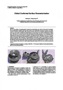
Fig. 2. (A) Conformal net and critical graph of a closed three-hole torus surface. There are four zero points. The critical horizontal trajectories partition the surface to four topological cylinders, color encoded in the third frame. Each cylinder is conformally mapped to a planar rectangle. (B) Conformal net and critical graph of a open boundary four-hole annulus on the plane. There are three zero points; the critical horizontal trajectories partition the surface to six topological disks. (C). Each segment is conformally mapped to a rectangle. The trajectories and the boundaries are color encoded and the corners are labelled. (Pictures are adapted from [29].)

then is still a holomorphic function. For a genus closed surface, all holomorphic 1-forms form a 2 real dimensional linear space. of a holomorphic 1-form , any local At a zero point parametric representation has

According to the Riemann–Roch theorem, in general there are 2 2 zero points for a holomorphic 1-form defined on a closed . surface of genus , where A holomorphic 1-form induces a special system of curves on a surface, the so-called conformal net. Horizontal trajectories are the curves that are mapped to iso-v lines in the parameter domain. Similarly, vertical trajectories are the curves that are mapped to iso-u lines in the parameter domain. The horizontal and vertical trajectories form a web on the surface. The trajectories that connect zero points, or a zero point with the boundary, are called critical trajectories. The critical horizontal trajectories form a graph, which is called the critical graph. In general, the behavior of a trajectory may be very complicated, may have

855

infinite length, and may be dense on the surface. If the critical graph is finite, then all the horizontal trajectories are finite. The critical graph partitions the surface into a set of nonoverlapping patches that jointly cover the surface, and each patch is either a topological disk or a topological cylinder [27]. Each can be mapped to the complex plane by the intepatch gration of holomorphic 1-form on it. The structure of the critical graph and the parameterizations of the patches are determined by the conformal structure of the surface. If two surfaces are topologically homeomorphic to each other and have similar geometrical structure,1 they can support consistent critical graphs and segmentations (i.e., surface partitions), and their parameterizations are consistent as well. Therefore, by matching their parameter domains, the entire surfaces can be directly matched in 3-D. This generalizes prior work in medical imaging that has matched surfaces by computing a smooth bijection to a single canonical surface, such as a sphere or disk. Fig. 2(A) and (B) shows the conformal net and critical graph on closed surface and open boundary surface, respectively. The surface segmentation results are also shown. Fig. 2(C) illustrates how a segment in (B) is conformally mapped to a rectangle. In (C), conformal nets are labeled with different colors. In the parameter domain, we can also find the right angles between the conformal net curves are well preserved. The zero point on the left is mapped to two points on the opposite edges. We call the process of finding the critical graph and segmentation as holomorphic flow segmentation, a process that is completely determined by the geometry of the surface and the choice of the holomorphic 1-form.2 Computing holomorphic 1-forms is equivalent to solving elliptic differential equations on the surfaces, and in general, elliptic differential operators are stable (their solutions tend to be smooth functions and the boundary conditions of the Dirichlet problem can be fulfilled). Therefore, the resulting surface segmentations and parameterizations are intrinsic and stable and are applicable for matching (potentially noisy) surfaces that are derived from medical images and topologically homeomorphic to each other [30] because the behavior of horizontal trajectory is solely determined by the conformal structure and the cohomology class of the holomorphic 1-form. In surface matching application, we guarantee that the cohomology classes are consistent on two surfaces and the two surfaces are with similar conformal structures, therefore, the corresponding trajectories will behave in the similar way. This paper takes advantage of conformal structures of surfaces, consistently segments them, and parameterizes the patches using a holomorphic 1-form. We then explore various applications that use the resulting parameterization. With the conformal parametrization, we can solve variational problems and PDEs on the surface, which describe either physical phenomena on the manifold or signal processing operations (regularization, surface matching) that can be formulated using PDEs. The basic idea is to map the surface conformally to a instead 2-D rectangle and solve the corresponding PDE on 1A possible metric to evaluate how similar two surfaces’ geometrical strucin [28]. tures are is proposed as E 2Note that this differs from the typical meaning of segmentation in medical imaging and is concerned with the segmentation, or partitioning, of a general surface.

856


of solving the PDE on the manifold. To do this, we have to use the manifold version of differential operators (tensor calculus). Using the conformal parametrization, these differential operators on the manifold can be described more easily on the paby simple formulas. This will be explained rameter domain briefly as below. be a manifold and be the global conLet formal parametrization of . With the conformal parametrization, we can do calculus on surfaces similar to what we do on . Suppose is a smooth map. We will first deof . On , we usually define the fine partial derivative partial derivative by taking the limit. For example, . With the conformal parametrization, we can define the partial derivative on scalar functions in the same manner. Because of the stretching effect, we define

where is the conformal factor. is defined similarly. , is characterized Now, the gradient of a function . Simple checking gives us by where is the inverse of the Riemannian . With the conformal parametrization, we can demetric fine the gradient of similar to the definition on . Namely

TABLE I LIST OF FORMULAS FOR SOME STANDARD DIFFERENTIAL OPERATORS ON GENERAL MANIFOLD

, where is called the direction of the differentiation. This operation is based on the tensor calculus [31]. , where is Given a Riemannian manifold the Riemannian metric, suppose is the coordinate basis of the vector field. A simple verification will tell us the covariant derivative can be calculated by the following formula:

(2) where

Suppose now that the parametrization is conformal. The Riemannian metric is simply , where are the conformal factor and the identity matrix respectively. We then have the following formula:

Suppose is a smooth function. With this definition of gradient, we still have the following useful fact as in :

Length of With this formula, we can calculate easily. More interesting formulas for the manifold differential operators [32] on the parameter domain can be found in Table I. II. HOLOMORPHIC FLOW SEGMENTATION

where is the delta function and is the Heaviside function. Next, we give a definition of a differential operator on a vector field. It can be done by the covariant differentiation

To compute the holomorphic flow segmentation of a surface, first we compute the conformal structure of the surface; then we select a holomorphic differential form and locate the zero points on it (details are given below). By tracing horizontal trajectories through the zero points, the critical graph can be constructed and


the surface is divided into several patches. Each patch can then be conformally mapped to a planar parallelogram by integrating the holomorphic differential form. In this paper, surfaces are represented as triangular meshes, namely, piecewise polygonal surfaces. The computations with differential forms are based on solving elliptic partial differential equations on surfaces using finite-element method. Supis a simplicial complex, and a mapping pose embeds in ; then is called a triangular , where are the sets of -simplices. We use mesh. to denote an -simplex, where . A. Computing Conformal Structures A method for computing the conformal structure of a surface is a closed genus was introduced in [33]. Suppose surface with a conformal atlas . The conformal structure induces holomorphic 1-forms; all holomorphic 1-forms form of dimension 2 over real numbers that a linear space is isomorphic to the first cohomology group of the surface . The set of holomorphic 1-forms determines the conformal structure. Therefore, computing conformal structure is equivalent to finding a basis for . of is comThe holomorphic 1-form basis puted as follows: compute the homology basis, find the dual cohomology basis, diffuse the cohomology basis to a harmonic 1-form basis, and then convert the harmonic 1-form basis to holomorphic 1-form basis by using the Hodge star operator. The details of the computation are given in [33].3 In terms of data structure, a holomorphic 1-form is represented as a vectorvalued function defined on the edges of the mesh . B. Canonical Conformal Parameterization Computation Given a Riemann surface , there are infinitely many holomorphic 1-forms, but each of them can be expressed as a linear combination of the basis elements. We define a canonical conformal parameterization as any linear combination of the set of , where . holomorphic basis functions , where are hoThey satisfy is the Kronecker symbol. Then we commology bases and . pute a canonical conformal parameterization We select a specific parameterization that maximizes the uniformity of the induced grid over the entire domain using the algorithms introduced in [34], for the purpose of locating zero points in the next step.

857

1) Estimating the Conformal Factor: Suppose we already have a global conformal parameterization, induced by a holomorphic 1-form . Then we can estimate the conformal factor at each vertex, using the following formulas:

(3) and are the set of 0-simplices and 1-simplices, where respectively; is the valence of vertex . 2) Locating Zero Points: We find the cluster of vertices with relatively small conformal factors (the lowest 5–6%). These are candidates for zero points. We cluster all the candidates using the metric on the surface. For each cluster, we pick the vertex that is on the surface and closest to the center of gravity of the cluster, using the surface metric to define geodesic distances. Because the triangulation is finite and the computation is an approximation, the number of zero points may not equal to the Euler number. In this case, we refine the triangulation of the neighborhood of the zero point candidate and refine the holomorphic 1-form .4 According to the Riemann surface theory, zero points are isolated in general. In very rare cases, zero points can be merged. However, the probability of those cases is zero. The configuration of zero points is completely determined by the cohomology class of the holomorphic 1-forms. By choosing cohomology class, we can control the distances among zero points. In practice, with topological optimization method [34], we can adaptively change the surface cohomology class of the holomorphic 1-form by changing the surface topological structure, e.g., cutting open surfaces along some feature lines. As shown in Fig. 2(b), by choosing the canonical conformal parameterization result, the zero points are well separated by the cutting curves. D. Holomorphic Flow Segmentation

For a close surface with genus , any holomorphic 1-form has 2 2 zero points. For an open boundary surface , any holomorphic 1-form has 1 zero with genus points. The horizontal trajectories through the zero points will partition the surface into several discrete patches. Each patch is either a topological disk or a cylinder and can be conformally parameterized by a parallelogram.

1) Tracing Horizontal Trajectories: Once the zero points are located, the horizontal trajectories through them can be traced. First we choose a neighborhood of a vertex , where represents a zero point and is a set of neighboring faces of . Then we map it to the parameter plane by integrating . Suppose a vertex and a path composed by a sequence of edges on . the mesh is ; then the parameter location of is The conformal parameterization is a piecewise linear map. Then the horizontal trajectory is mapped to the horizontal in the parameter domain. We slice line using the line by edge splitting operations. Supintersects constant at a point pose the boundary of ; then we choose a neighborhood of and repeat the process. Each time we extend the horizontal trajectory and encounter edges intersecting the trajectory. We insert new vertices at the intersection points, until the trajectory reaches another zero point (for a closed surface) or the boundary of the mesh (for an open boundary surface). Each zero point connects to four

3For surfaces with boundaries, we apply the conventional double covering technique, which glues two copies of the same surface along their corresponding boundaries to form a symmetric closed surface. Then we apply the above procedure to find the holomorphic 1-form basis.

4It is worth noting that the same research group has proposed to use a new mathematical tool, the Ricci flow, to eliminate the numerical errors in the zero point location computation [35]. The detailed development will be reported in our future work.

C. Locating Zero Points

858


horizontal trajectories, and the angles between two adjacent trajectories are right angles. In practice, we just trace four trajectories starting from each zero point to guarantee to have all the trajectories. 2) Critical Graph: Given a surface and a holomorphic as 1-form on , we define the graph the critical graph of , where is the set of zero points of is the set of horizontal trajectories connecting zero points or the boundary segments of , and is the set of surface patches segmented by . Given two surfaces that are topologically homeomorphic to each other and have similar geometrical structures, by choosing the canonical holomorphic 1-forms, we can obtain isomorphic critical graphs, which can be used for surface matching [30].

III. AUTOMATIC LANDMARK TRACKING WITH RIEMANN SURFACE STRUCTURE Finding important feature points or curves on anatomical surfaces, such as sulcal/gyral curves on the cortical surface, is an important problem in medical imaging. These cortical landmarks provide important features for the neuroscientific study of brain diseases, or they can be used as geometrical constraints to help guide the matching of different cortical surfaces [2], [36]–[38]. Although the sulci do not represent an absolute guide to functional homology in the cortex, in the absence of additional histologic information they are often used as constraints when spatially normalizing anatomy of different subjects to match a common brain template. Using the Riemann surface structure, we propose a variational method to identify and track landmark curves on cortical surfaces automatically based on the principal directions, which were also used by other works [39], [40]. Suppose we are given the conformal parameterization of a cortical surface; our method traces the landmark curves iteratively on the spherical/rectangular parameter domain along the principal direction. The principal directions are, by definition, the eigenvectors of the Weingarten (curvature) matrix. Consequently, the landmark curves can be mapped onto the cortical surface. To speed up the iterative scheme, we propose a method to get a good initialization by extracting high mean curvature regions on the cortical surface using the Chan–Vese (CV) segmentation method, which involves solving a PDE on the manifold using our conformal parametrization technique.

A. Variational Method for Landmark Tracking Consider the principal direction field with smaller eigenvalues of the curvature matrix on the cortical surface . Fixing two anchor points on the sulci, we propose a variational method to trace the sulcal landmark curve iteratively. Let be the conformal parametrization of , be its Riemannian metric, and be its conformal factor. We propose

with endpoints to locate a curve minimizes the following energy functional:

where

and , which

is the corresponding iterative

curve on the parameter domain; ; ; and is the (usual) length defined on . By minimizing the energy , we minimize the difference between the tangent vector field along the curve and the principal direction field . The resulting minimizing curve is the curve that is closest to the curve traced along the principal direction. Let ; ; . We can locate the landmark curves iteratively using the steepest descent algorithm

B. Landmark Hypothesis Generation by the Chan–Vese Segmentation In order to speed up the iterative scheme, we obtain a good initialization by extracting the high mean curvature regions on the cortical surface using the CV segmentation method [41]. Based on techniques of curve evolution, Mumford–Shah functional [42] for segmentation, and level sets, the CV model is a widely used 2-D image segmentation method. With our conformal parameterization, we extend the CV segmentation on to any arbitrary Riemann surface such as the cortical surface. be the conformal parametrization of the surLet face . We propose to minimize the following energy functional:


859

where is the level set function and and is the mean curvature function on the cortical surface. With the conformal parametrization, we have

For simplicity, we let we must have

Fixing

and

. Fixing ,

, the Euler–Lagrange equation becomes

Locating sulcal landmark features using geometric properties of the anatomical features has been widely studied [39], [40], [43]–[48]. In general, sulcal landmarks on the cortex lie in regions with relatively high mean curvature [49], [50]. Using the CV segmentation, we can consider the signal of interest, defined on the cortex, as the mean curvature. The sulci position on the cortical surface can then be located by extracting out the high curvature region. Inside each region, a good initialization of the landmark curve is considered as the shortest path that connects two anchor points when the region is considered as a graph. We select two umbilic points as the anchor points. By definition, an umbilic point on a manifold is a location at which the two principal curvatures are the same. If there are multiple umbilic points are found in one region, we select the two that are furthest apart. IV. OPTIMIZATION OF BRAIN CONFORMAL MAPPING USING SULCAL LANDMARKS In brain-mapping research, cortical surface data are often mapped conformally to a parameter domain such as a sphere, providing a common coordinate system for data integration [13], [17], [51]. As an application of our automatic landmark tracking algorithm, we use the automatically labelled landmark curves to generate an optimized conformal mapping on the surface. This matching of cortical patterns improves the alignment of data across subjects. It is done by minimizing the compound energy functional

Fig. 3. The holomorphic flow segmentation results of (a)–(d) a hippocampal surface and (e)–(l) two lateral ventricular surfaces. (b) is the conformal net of the hippocampal surface in (a). (c) is an isoparameter curve used to unfold the surface. (d) is the rectangle to which the surface is conformally mapped. (e)–(h) show lateral ventricles parameterized using holomorphic 1-forms for a 65-year-old subject with HIV/AIDS; (i)–(l) show the same maps computed for a healthy 21-year-old control subject. (e) and (i) show that five cuts are automatically introduced and convert the lateral ventricular surface into a genus 4 surface. Other pictures show the (f) and (j) computed conformal net, (g) and (k) holomorphic flow segmentation, and (h) and (l) their associated parameter domains (the texture mapped into the parameter domain here simply corresponds to the intensity of the surface rendering, which is based on the surface normals).

where zation [13] and

is the harmonic energy of the parameteri-

is the landmark mismatch energy [52], where the norm represents distance between automatic traced landmark curves and , represented on the parameter domain . Here, automatically traced landmark (continuous) curves are used and the correspondence is obtained on the curves using the unit length and unit speed reparametrization. We can minimize the energy by steepest descent method. The resulting brain conformal mapping improves cortical surface registration significantly while preserving conformality to the highest possible degree [52]. Note that we may also describe the landmark matching problem on the sphere within the large deformation diffeomorphism framework [53]. V. EXPERIMENTAL RESULTS A. Hippocampal Surface Parameterization Fig. 3(a)–(d) shows experimental results for a hippocampal surface, a structure in the medial temporal lobe of the brain. The original surface is shown in (a). We leave two holes at the front and back of the hippocampal surface, representing its anterior junction with the amygdala and its posterior limit as it

860


turns into the white matter of the fornix. The hippocampus can be logically represented as an open boundary genus one surface, i.e., a cylinder (note that spherical harmonic representations would also be possible if the ends were closed [54]–[57]). The computed conformal net is shown in (b), where the red and blue curves are the vertical trajectories and the horizontal trajectories of the net, respectively. A horizontal trajectory curve is shown in (c). Cutting the surface along this curve, we can then conformally map the hippocampus to a rectangle. The detailed surface information is well preserved in (d). Compared with other spherical parameterization methods, which may have high-valence nodes and dense tiles at the poles of the spherical coordinate system, our parameterization can represent the surface with minimal distortion.5 B. Lateral Ventricular Surface Parameterization Shape analysis of the lateral ventricles—a fluid-filled structure deep in the brain—is of great interest in the study of psychiatric illnesses, including schizophrenia [58], [59], and in degenerative diseases such as Alzheimer’s disease [60], [61]. These structures are often enlarged in disease and can provide sensitive measures of disease progression. To model the lateral ventricular surface in each brain hemisphere, we introduce five cuts. Although this seems arbitrary, the cuts are motivated by examining the topology of the lateral ventricles, in which several horns are joined together at the ventricular “atrium” or “trigone.” We call this topological change topological optimization. The topological optimization helps to get a uniform parameterization on some areas that otherwise are very difficult for usual parameterization methods to capture. A systematic topological optimization method was introduced in [34]. With this method, we automatically located initial points, which are simply the extremal points of the anterior/posterior coordinate, for these cuts at a specific set of extreme points. Specifically, they are at the ends of the frontal, occipital, and temporal horns of the ventricles. Fig. 3(e) and (i) shows five cuts introduced on two subjects’ ventricular surfaces. After the cutting, the surfaces become open-boundary genus 4 surfaces. The rest of Fig. 3 shows parameterizations of the lateral ventricles of the brain. Fig. 3(e)–(h) shows the results of parameterizing a ventricular surface for a 65-year-old patient with HIV/AIDS (note the disease-related enlargement) and Fig.3 (i)–(l) shows the results for the ventricular model of a 21-year-old control subject (surface data are from [60]). The computed conformal structures are shown in Fig. 3(f) and (j) by texture mapping a checkerboard image to the surface. There are a total of three zero points on each of the ventricular surfaces. Two of them are located at the middle part of the two “arms” (where the temporal and occipital horns join at the ventricular atrium), as shown by the large black dots in (f) and (j). The third zero point is located in the middle of the model, where the frontal horns are closest to each other. Based on the computed conformal structure, we can partition the surface into six patches. Each patch can be 5When matching two hippocampal surfaces with our conformal parameterization, we need to find a consistent trajectory to cut them open. A possible way to do it is to use principal axis registration first, i.e., get the inertia matrix of one surface and apply its inverse to the other one. After that, we can find a consistent trajectory that guarantees the cutting results have consistent boundaries.

Fig. 4. Illustrates the parameterization of cortical surfaces using the holomorphic 1-form approach. The thick lines are landmark curves, including several major sulci lying in the cortical surface. These sulcal curves are always mapped to a boundary in the parameter space images.

conformally mapped to a rectangle. Although the two brain ventricle shapes are very different, the segmentation results are consistent in that the surfaces are partitioned into patches with the same relative arrangement and connectivity. Thus our method provides a basis to perform direct surface matching between any two ventricles. Note that this is somewhat a different approach to surface matching than those typically adopted. Rather than use a single parameterization for the entire surface, and match landmarks that lie within it, instead a topological decomposition of the surface is used and the patches are piecewise matched and guaranteed to be conformal. The advantage of this approach is that it can handle the matching of objects with nonspherical (but consistent) topology, which would otherwise be extremely difficult to parameterize and match. C. Cerebral Cortical Surface Parameterization For the surface of the cerebral cortex, our algorithm also provides a way to perform surface matching while explicitly matching sulcal curves or other landmarks lying in the surface. Note that typically two surfaces can be matched by using a landmark-driven flow in their parameter spaces [2], [13], [17], [62], [63]. An alternative approach is to supplement the critical graph with curved landmarks that can then be forced to lie on the boundaries of rectangles in the parameter space. This has the advantage that conformal grids are still available on both surfaces, as is a correspondence field between the two conformal grids. Fig. 4 shows the results for the cortical surfaces of two left hemispheres. As shown in the first row, we selected four major landmark curves, for the purpose of illustrating


the approach (thick lines show the precental and postcentral sulci, and the superior temporal sulcus, and the perimeter of the corpus callosum at the midsagittal plane). By cutting the surface along the landmark curves, we obtain a genus 3 open boundary surface. The conformal structure is illustrated by texture mapping a checkerboard image to the cortical surface (the first panel of the first row). There are therefore two zero points (observable as a large white region and black region in the conformal grid). We show cortical surfaces from two different subjects in Fig. 4 (these are extracted using a deformable surface approach but are subsequently reparameterized using holomorphic 1-forms). The second and fourth rows show the segmented patches for each cortical surface. The rectangles that these patches conformally map to are shown on the third and fifth row, respectively. Since the landmark curves lie on the boundaries of the surface patches, they can be forced to lie on an isoparameter curve and can be constrained to map to rectangle boundaries in the parameter domain. Although the two cortical surfaces are different, the selected sulcal curves are mapped to the rectangle boundaries in the parameter domain. This method therefore provides a way to warp between two anatomical surfaces while exactly matching an arbitrary number of landmark curves lying in the surfaces. As in prior work, this is applicable to tracking brain growth or degeneration in serial scans, and composite maps of the cortex can be made by invoking the consistent parameterizations [64]–[66]. Thiron’s extremal mesh [40] and the work of Lamecker et al. on the cortex [67] have a similar motivation to ours, namely, to partition a surface into canonical patches and parameterize the patches with minimal distortion. However, our partitioning method is based on intrinsic Riemann surface structure and theirs is based on shortest paths along lines of high curvature. In our method, the segmentation and parameterizations are solely determined by the conformal structure of the surface, which is determined by the Riemannian metric and independent of the embedding. It is invariant under isometric transformation and conformal transformation. Thus, our method is global and may be more stable. D. Automatic Landmark Location With Riemann Surface Structure As for our automatic landmark location algorithm, we tested the algorithm on a set of left hemisphere cortical surfaces extracted from brain magnetic resonance imagin scans, acquired from normal subjects at 1.5 T (on a GE Signa scanner) [68]. In our experiments, ten landmarks were automatically located on cortical surfaces. Fig. 5(A)–(D) shows how we can effectively locate the initial estimated landmark regions on the cortical surface using the CV segmentation approach in the parameter domain. Notice that the contour evolved to the deep sulcal region. In Fig. 5(E), we locate two umbilic points in each sulcal region. When multiple umbilic points are located in a region, we select the two that are farthest apart. The selected umbilic points are chosen as the anchor points for variational landmark tracing step. Our variational method to locate landmark curves is illustrated in Fig. 5(F)–(H). With the initial guess given by the CV

861

Fig. 5. (A)–(D) show sulcal curve extraction on the cortical surface by the CV segmentation. With a suitable initial contour, major sulcal landmarks can be effectively extracted at the same time. (E) shows how umbilic points are located within each candidate sulci region, and these are then chosen as the end points of the landmark curves. When multiple candidates regions are located, we select the two regions that are farthest apart. (F)–(H) illustrate automatic landmark tracking using a variational approach. In (F), we track the landmark curves on the parameter domain along the edges whose directions are closest to the principal direction field. The corresponding landmark curves on the cortical surface are shown. This gives a good initialization for our variational method to locate landmarks. (G) demonstrates that landmarks curve is evolved to a deeper region using our variational approach. The blue and green curves represents the initial and evolved curves, respectively. (H) shows ten sulci landmarks that are detected and tracked using our algorithm.

model (we choose the two extreme umbilic points in the located area as the anchor points), we trace the landmark curves iteratively based on the principal direction field. In Fig. 5(F), we trace the landmark curves on the parameter domain along the edges whose directions are closest to the principal direction field. The corresponding landmark curves on the cortical surface is shown. Fig. 5(G) shows how the curve evolves to a deeper sulcal region with our iterative scheme. In Fig. 5(H), ten sulci landmarks are located using our algorithm. E. Optimization of Brain Conformal Parametrization To visualize how well our optimized brain conformal parametrization algorithm can improve the alignment of key sulci landmarks, we created an average 3-D surface based on the 15 optimized conformal maps. Namely, we took the average geometric positions of every corresponding vertex on 15 cortical surfaces. Fig. 6 shows average maps from different angles. In (B) and (C), sulci landmarks are clearly preserved inside the green circle where landmarks are manually labelled. In (D), the sulci landmarks are averaged out inside the green circle where no landmarks are automatically detected. This suggests that

862


well as brain surface registration with surface metric proposed in [30], and shape and asymmetry analysis for subcortical structures. APPENDIX A Claim 1: Suppose

is a smooth function. Then

Proof: Recall that the Co-area formula reads

Fig. 6. An average cortical surface of the brain derived by using optimized conformal parametrization with the automatically traced landmarks. The major sulcal landmarks are well preserved (see the areas inside green circles in (B) and (C). In (D), the sulci at the back of the brain, in the occipital lobe surface, are averaged out because no landmark constraint was added in that region, for purposes of illustration.

where is the Hausdorff measure. Let be the conformal parametrization of the surface . Then

and

our algorithm can help by improving the alignment of major anatomical features in the cortex. Further validation work, of course, would be necessary to assess whether this results in greater detection sensitivity in computational anatomy studies of the cortex, but the greater reinforcement of features suggests that landmark alignment error is substantially reduced, and this is one major factor influencing signal detection in multisubject cortical studies. VI. CONCLUSION AND FUTURE WORK In this paper, we presented a brain surface parameterization method that invokes the Riemann surface structure to generate conformal grids on surfaces of arbitrary complexity (including branching topologies). For high genus surfaces, a global conformal parameterization induces a canonical segmentation, i.e., there is a discrete partition of the surface into conformally parameterized patches. We tested our algorithm on hippocampal and lateral ventricular surfaces and on surface models of the cerebral cortex. The grid generation algorithm is intrinsic (i.e., it does not depend on any initial choice of surface coordinates) and is stable, as shown by grids induced on ventricles of various shapes and sizes. With the conformal parameterization, we employed a set of formulas for the covariant differential operators on the manifold based on tensor calculus. Because of this conformal parameterization, the extension of well-known 2-D PDE solvers to general 3-D surfaces becomes relatively simple. We illustrate the use of the conformal grid for hosting a surface-based PDE by presenting a brain landmark detection algorithm. The landmark detection results are examined by computing an average cortical surface after conformal parameterizations are optimized using sulcal features as landmarks. Our future work will focus on signal processing on brain surfaces, as

where

is the parametrization of

.

Q.E.D.

APPENDIX B . The geodesic curvature . Proof: Recall that the geodesic curvature of a curve

Case 2: Let

Let the parametrization of the zero level set of . Then . This implies

and

be

of is


863

Now

Thus, for conformal parametrization, we have

(4) Q.E.D.

and REFERENCES

(5) Combining these, we have

and

So

[1] P. M. Thompson, J. N. Giedd, R. P. Woods, D. MacDonald, A. C. Evans, and A. W. Toga, “Growth patterns in the developing human brain detected using continuum-mechanical tensor mapping,” Nature, vol. 404, no. 6774, pp. 190–193, Mar. 2000. [2] P. M. Thompson, R. P. Woods, M. S. Mega, and A. W. Toga, “Mathematical/computational challenges in creating deformable and probabilistic atlases of the human brain,” Human Brain Map., vol. 9, no. 2, pp. 81–92, Feb. 2000. [3] Y. Wang, M.-C. Chiang, and P. M. Thompson, “Automated surface matching using mutual information applied to Riemann surface structures,” in Proc. Med. Image Comp. Comput.-Assist. Intervention Part II, Palm Springs, CA, Oct. 2005, pp. 666–674. [4] S. Osher and J. A. Sethian, “Fronts propoagating with curvature dependent speed: Algorithms based on Hamilton-Jacobi formulations,” J. Comput. Phys., vol. 79, pp. 12–49, 1988. [5] F. Mémoli, G. Sapiro, and P. Thompson, “Implicit brain imaging,” NeuroImage, vol. 23, pp. S179–S188, 2004. [6] E. Schwartz, A. Shaw, and E. Wolfson, “A numerical solution to the generalized mapmaker’s problem: Flattening nonconvex polyhedral surfaces,” IEEE Trans. Pattern Anal. Machine Intell., vol. 11, no. 9, pp. 1005–1008, Sep. 1989. [7] B. Timsari and R. M. Leahy, “An optimization method for creating semi-isometric flat maps of the cerebral cortex,” presented at the SPIE Med. Imag., San Diego, CA, Feb. 2000. [8] H. A. Drury, D. C. V. Essen, C. H. Anderson, C. W. Lee, T. A. Coogan, and J. W. Lewis, “Computerized mappings of the cerebral cortex: A multiresolution flattening method and a surface-based coordinate system,” J. Cogn. Neurosci., vol. 8, pp. 1–28, 1996. [9] G. J. Carman, H. Drury, and D. C. V. Essen, “Computational methods for reconstructing and unfolding of primate cerebral cortex,” Cerebral Cortex, vol. 5, pp. 506–517, 1995. [10] M. K. Hurdal and K. Stephenson, “Cortical cartography using the discrete conformal approach of circle packings,” NeuroImage, vol. 23, pp. S119–S128, 2004. [11] K. Stephenson, Introduction to Circle Packing. Cambridge, U.K.: Cambridge Univ. Press, Apr. 2005. [12] S. Haker, S. Angenent, A. Tannenbaum, R. Kikinis, G. Sapiro, and M. Halle, “Conformal surface parameterization for texture mapping,” IEEE Trans. Vis. Comput. Graphics, vol. 6, no. 2, pp. 181–189, Apr. –Jun. 2000. [13] X. Gu, Y. Wang, T. F. Chan, P. M. Thompson, and S.-T. Yau, “Genus zero surface conformal mapping and its application to brain surface mapping,” IEEE Trans. Med. Imag., vol. 23, no. 8, pp. 949–958, Aug. 2004. [14] L. Ju, J. Stern, K. Rehm, K. Schaper, M. K. Hurdal, and D. Rottenberg, “Cortical surface flattening using least squares conformal mapping with minimal metric distortion,” in Proc. IEEE Int. Symp. Biomed. Imag.: From Nano to Macro, Arlington, VA, 2004, pp. 77–80. [15] A. A. Joshi, R. M. Leahy, P. M. Thompson, and D. W. Shattuck, “Cortical surface parameterization by p-harmonic energy minimization,” in Proc. IEEE Int. Symp. Biomed. Imag.: From Nano to Macro, Arlington, VA, 2004, pp. 428–431. [16] L. Ju, M. K. Hurdal, J. Stern, K. Rehm, K. Schaper, and D. Rottenberg, “Quantitative evaluation of three surface flattening methods,” NeuroImage, vol. 28, no. 4, pp. 869–880, 2005.

864


[17] B. Fischl, M. I. Sereno, and A. M. Dale, “Cortical surface-based analysis II: Inflation, flattening, and a surface-based coordinate system,” NeuroImage, vol. 9, pp. 179–194, 1999. [18] G. Turk, “Generating textures on arbitrary surfaces using reaction-diffusion,” Comput. Graph., vol. 25, no. 4, pp. 289–298, 1991. [19] J. Dorsey and P. Hanrahan, “Digital materials and virtual weathering,” Sci. Amer., vol. 282, no. 2, pp. 46–53, 2000. [20] J. Stam, “Flows on surfaces of arbitrary topology,” ACM Trans. Graph., vol. 22, no. 3, pp. 724–731, 2003. [21] U. Clarenza, M. Rumpfa, and A. Teleaa, “Surface processing methods for point sets using finite elements,” Comput. Graph., vol. 28, no. 6, pp. 851–868, 2004. [22] M. Bertalmio, L.-T. Cheng, S. Osher, and G. Sapiro, “Variational problems and partial differential equations on implicit surfaces,” J. Comput. Phys., vol. 174, no. 2, pp. 759–780, Dec. 2001. [23] M. Chung and J. Taylor, “Diffusion smoothing on brain surface via finite element method,” in Proc. IEEE Int. Symp. Biomed. Imag.: From Nano to Macro, Arlington, VA, 2004, pp. 432–435. [24] A. A. Joshi, D. W. Shattuck, P. M. Thompson, and R. M. Leahy, “A framework for registration, statistical characterization and classification of cortically constrained functional imaging data,” in Proc. Int. Conf. Inf. Process. Med. Imag., 2005, pp. 186–196. [25] W. M. Boothby, An Introduction to Differentiable Manifolds and Riemannian Geometry, 2nd ed. Orlando, FL: Academic, 1986. [26] J. Jost, Compact Riemann Surfaces: An Introduction to Contemporary Mathematics. Berlin, Germany: Springer-Verlag, 1997. [27] K. Strebel, Quadratic Differentials. Berlin, Germany: SpringerVerlag, 1984. [28] H. Hoppe, T. DeRose, T. Duchamp, J. McDonald, and W. Stuetzle, “Mesh optimization,” Comput. Graph., ser. Annu. Conf. Series, vol. 27, pp. 19–26, 1993. [29] Y. Wang, M. Jin, S.-T. Yau, and X. Gu, “Parameterize surfaces by surfaces,” presented at the ACM Solid Physical Modeling Symp., Beijing, China, Jun. 4–6, 2007. [30] Y. Wang, X. Gu, K. M. Hayashi, T. F. Chan, P. M. Thompson, and S.-T. Yau, “Surface parameterization using Riemann surface structure,” in Proc. 10th IEEE Int. Conf. Comput. Vision, Beijing, China, Oct. 2005, pp. 1061–1066. [31] J. Syngen and A. Schild, Tensor Calculus. London, U.K.: Dover, 1949. [32] L. Lui, Y. Wang, and T. F. Chan, “Solving PDEs on manifolds using global conference parametrization,” in VLSM, ICCV, Beijing, China, Oct. 16, 2005. [33] X. Gu and S.-T. Yau, “Computing conformal structures of surfaces,” Commun. Inf. Syst., vol. 2, no. 2, pp. 121–146, Dec. 2002. [34] M. Jin, Y. Wang, S.-T. Yau, and X. Gu, “Optimal global conformal surface parameterization for visualization,” in Proc. IEEE Visualization, Austin, TX, Oct. 2004, pp. 267–274. [35] Y. Wang, X. Gu, T. F. Chan, P. M. Thompson, and S.-T. Yau, “Brain surface conformal parameterization with algebraic functions,” in Proc. Med. Image Comp. Comput.-Assist. Intervention, Copenhagen, Denmark, Oct. 2006, pp. 946–854. [36] L. G. Goualher, E. Procyk, D. Collins, C. B. R. Venugopal, and A. Evans, “Automated extraction and variability analysis of sulcal neuroanatomy,” IEEE Trans. Med. Imag., vol. 18, no. 3, pp. 206–217, Mar. 1999. [37] A. Klein, J. Hirsch, S. Ghosh, J. Tourville, and J. Hirsch, “Mindboggle: A scatterbrained approach to automate brain labeling,” NeuroImage, vol. 24, no. 2, pp. 261–280, 2005. [38] P. Fillard, V. Arsigny, X. Pennec, K. M. Hayashi, P. M. Thompson, and N. Ayache, Measuring brain variability by extrapolating sparse tensor fields measured on sulcal lines Res. Rep. INRIA 5887, Apr. 2007. [39] M. Fidrich, “Iso-surface extraction in nD applied to tracking feature curves across scale,” Image Vision Comput., vol. 16, no. 8, pp. 545–556, 1998. [40] J.-P. Thirion, “The extremal mesh and the understanding of 3D surfaces,” Int. J. Comput. Vision, vol. 19, no. 2, pp. 115–128, 1996. [41] L. A. Vese and T. F. Chan, “Multiphase level set framework for image segmentation using the Mumford and Shah model,” Int. J. Comput. Vision, vol. 50, no. 3, pp. 271–293, 2002. [42] D. Mumford and J. Shah, “Optimal approximations by piecewise smooth functions and associated variational problems,” Commun. Pure Appl. Math., vol. 42, no. 5, pp. 577–685, 1989. [43] M. E. Rettmann, D. Tosun, X. Tao, S. M. Resnick, and J. L. Prince, “Program for the assisted labeling of sulcal regions (PALS): Description and validation,” NeuroImage, vol. 24, no. 2, pp. 398–416, 2005.

[44] M. Rettman, X. Han, and J. L. Prince, “Automated sulcal segmentation using watersheds on the cortical surface,” NeuroImage, vol. 15, no. 2, pp. 329–344, 2002. [45] G. Lohmann, F. Kruggel, and D. von Cramon, “Automatic detection of sulcal bottom lines in MR images of the human brain,” Inf. Process. Med. Imag., vol. 1230, pp. 368–374, 1997. [46] D. Rey, G. Subsol, H. Delingette, and N. Ayache, “Automatic detection and segmentation of evolving processes in 3D medical images: Application to multiple sclerosis,” Med. Image Anal., vol. 6, no. 2, pp. 163–179, Jun. 2002. [47] N. Khaneja, M. Miller, and U. Grenander, “Dynamic programming generation of curves on brain surfaces,” IEEE Trans. Pattern Anal. Machine Intell., vol. 20, no. 11, pp. 1260–1265, Nov. 1998. [48] X. Zeng, L. Staib, R. Schultz, L. Win, and J. Duncan, “A new approach to 3D sulcal ribbon finding from MR images,” in Proc. Med. Image Comp. Comput.-Assist. Intervention, 1999, pp. 148–157. [49] A. Cachia, J.-F. Mangin, D. Rivire, N. Boddaert, A. Andrade, F. Kherif, P. Sonigo, D. Papadopoulos-Orfanos, M. Zilbovicius, J.-B. Poline, I. Bloch, F. Brunelle, and J. Rgis, “A mean curvature based primal sketch to study the cortical folding process from antenatal to adult brain,” in Proc. Med. Image Comp. Comput.-Assist. Intervention, Oct. 2001, vol. 2208, pp. 897–904. [50] C. Kao, M. Hofer, G. Sapiro, J. Stern, and D. Rottenberg, “A geometric method for automatic extraction of sulcal fundi,” in Proc. IEEE Int. Symp. Biomed. Imag.: From Nano to Macro, Apr. 2006, pp. 1168–1171. [51] H. A. Drury, D. C. V. Essen, M. Corbetta, and A. Z. Snyder, “Surfacebased analyses of the human cerebral cortex,” in Brain Warping. New York: Academic, 1999. [52] Y. Wang, L. M. Lui, T. F. Chan, and P. M. Thompson, “Optimization of brain conformal mapping with landmarks,” in Proc. Med. Image Comp. Comput.-Assist. Intervention Part II, Oct. 2005, pp. 675–683. [53] A. Leow, C. L. Yu, S. J. Lee, S. C. Huang, H. Protas, R. Nicolson, K. M. Hayashi, A. W. Toga, and P. M. Thompson, “Brain structural mapping using a novel hybrid implicit/explicit framework based on the level-set method.,” NeuroImage, vol. 24, pp. 910–927, 2005. [54] A. Kelemen, G. Székely, and G. Gerig, “Elastic model-based segmentation of 3D neuroradiological data sets,” IEEE Trans. Med. Imag., vol. 18, no. 10, pp. 828–839, Oct. 1999. [55] M. Styner, J. A. Lieberman, D. Pantazis, and G. Gerig, “Boundary and medial shape analysis of the hippocampus in schizophrenia,” Med. Image Anal., vol. 8, no. 3, pp. 197–203, 2004. [56] J. G. Csernansky, L. Wang, D. Jones, D. Rastogi-Cruz, J. A. Posener, G. Heydebrand, J. P. Miller, and M. I. Miller, “Hippocampal deformities in Schizophrenia characterized by high dimensional brain mapping,” Amer. J. Psych., vol. 159, pp. 2000–2006, Apr. 2002. [57] B. Gutman, Y. Wang, L. M. Lui, T. F. Chan, and P. M. Thompson, “Hippocampal surface analysis using spherical harmonic function applied to surface conformal mapping,” Proc. Int. Conf. Pattern Recognit., vol. 3, pp. 964–967, 2006. [58] K. L. Narr, P. M. Thompson, T. Sharma, J. Moussai, R. E. Blanton, B. Anvar, A. Edris, R. Krupp, J. Rayman, M. Khaledy, and A. W. Toga, “3D mapping of temporo-limbic regions and the lateral ventricles in schizophrenia,” Biol. Psych., vol. 50, pp. 84–97, 2001. [59] G. Gerig, M. Styner, D. Jones, D. Weinberger, and J. Lieberman, “Shape analysis of brain ventricles using SPHARM,” in Proc. IEEE Comput. Soc. MMBIA 2001, Dec. 2001, pp. 171–178. [60] P. M. Thompson, R. A. Dutton, K. M. Hayashi, A. Lu, S. E. Lee, J. Y. Lee, O. L. Lopez, H. J. Aizenstein, A. W. Toga, and J. T. Becker, “3D mapping of ventricular and corpus callosum abnormalities in HIV/ AIDS,” NeuroImage, to be published. [61] O. T. Carmichael, P. M. Thompson, R. A. Dutton, A. Lu, S. E. Lee, J. Y. Lee, L. H. Kuller, O. L. Lopez, H. J. Aizenstein, C. C. Meltzer, Y. Liu, A. W. Toga, and J. T. Becker, “Diffusion smoothing on brain surface via finite element method,” in IEEE Int. Symp. Biomed. Imag.: From Nano to Macro, Arlington, VA, 2006, pp. 315–318. [62] P. M. Thompson and A. W. Toga, “A surface-based technique for warping 3-dimensional images of the brain,” IEEE Trans. Med. Imag., vol. 15, no. 4, pp. 1–16, 1996. [63] C. Davatzikos, “Spatial normalization of 3D brain images using deformable models,” Comput. Assist. Tomogr., vol. 20, no. 4, pp. 656–665, 1996. [64] P. M. Thompson, C. N. Vidal, J. N. Giedd, P. Gochman, J. Blumenthal, R. Nicolson, A. W. Toga, and J. L. Rapoport, “Mapping adolescent brain change reveals dynamic wave of accelerated gray matter loss in very early-onset schizophrenia,” in Proc. Nat. Acad. Sci., Sep. 2001, vol. 98, no. 20, pp. 11650–11655.


[65] P. M. Thompson, K. M. Hayashi, G. de Zubicaray, A. L. Janke, S. E. Rose, J. Semple, D. Herman, M. S. Hong, S. Dittmer, D. M. Doddrell, and A. W. Toga, “Dynamics of gray matter loss in Alzheimer’s disease,” J. Neurosci., vol. 23, no. 3, pp. 994–1005, Feb. 2003. [66] N. Gogtay, J. N. Giedd, L. Lusk, K. M. Hayashi, D. Greenstein, C. Vaitiuzis, T. F. Nugent, D. H. Herman, L. Classen, A. W. Toga, J. L. Rapoport, and P. M. Thompson, “Dynamic mapping of human cortical development during childhood and adolescence,” in Proc. Nat. Acad. Sci., May 2004, vol. 101, no. 21, pp. 8274–8179.

865

[67] H. Lamecker, T. Lange, and M. Seebass, “A statistical shape model for the liver,” Med. Image Comp. Comput.-Assist. Intervention, pp. 422–427, Sep. 2002. [68] P. M. Thompson, A. D. Lee, R. A. Dutton, J. A. Geaga, K. M. Hayashi, M. A. Eckert, U. Bellugi, A. M. Galaburda, J. R. Korenberg, D. L. Mills, A. W. Toga, and A. L. Reiss, “Abnormal cortical complexity and thickness profiles mapped in Williams syndrome,” J. Neurosci., vol. 25, no. 16, pp. 4146–4158, Apr. 2005.