Color texture segmentation for clothing in a computer ... - CiteSeerX

y?J VISI n ELSEVIER

Image and Vision Computing 14 (1996) 685-702

Application

note

Color texture segmentation for clothing in a computer-aided design system Chin-Chou Department

Chang,

Ling-Ling

of Computer Science, National Tsing Hua University,

fashion

Wang* Hsinchu, 30043 Taiwan, ROC

Received 4 July 1995; revised 11 December 1995

Abstract A traditional fashion designer has to draw a large number of drafts in order to accomplish an ideal style. Better performance can be achieved if these operations are done on computers, because the designer can easily make changes for various patterns and colors. To develop a computer-aided fashion design system, one of the most difficult tasks is to automatically separate the clothing from the background so that a new item can be ‘put on’. One difficulty of the segmentation work arises from the diverse patterns on the clothing, especially with folds or shadows. In this study, circular histograms are first utilized to quantize color and to reduce shadow/ highlight effects. Then a color co-occurrence matrix and a color occurrence vector are proposed to characterize the color spatial dependence and color occurrence frequency of the clothing’s texture. Next, based on the two color features blocks on the clothing are found by a region growing method. Finally, post-processing is applied to obtain a smooth clothing boundary. Experimental results are presented to show the feasibility of the proposed approach. Keywords: Image segmentation; Color quantization; Color co-occurrence matrix; Computer-aided

1. Introduction 1.1. Research

motivation

A traditional fashion designer has to draw a large number of drafts in order to accomplish an ideal style. Hence, an effective tool which can provide a realistic customer model, and by which a large amount of drawing time can be saved, is very helpful for a fashion designer. Due to the rapid development of computer software, a computer-aided fashion design system now becomes feasible. By inputting a customer’s photographs to a computer, a designer can take the customer as a model. Further, through the computer program’s cut & paste commands (functions), when the colors or pattern prints of the the designed clothing are to be modified, it is not necessary to redraw a new draft. Only the part to be modified is cut and pasted on the computer. Therefore, much drawing work on paper can be saved, and the best selection of colors or patterns on the clothing designed

* Corresponding author. 0262~8856/96/$15.00 0 1996 Elsevier Science B.V. All rights reserved PZZ SO262-8856(96)01083-9

fashion design

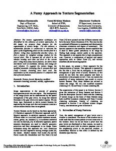
can be determined quickly according to the customer model. Better performance can thus be achieved. For a computer-aided fashion design system, one of the most difficult tasks is to automatically cut or separate the clothing to be modified from its background so that the clothing can be ‘taken off’, and a new item with different colors, patterns or even new styles can be ‘put on’ to the model. Few commercial image processing or image editing packages perform segmentation well. For some packages the users even have to specify by hand the boundary of the clothing on the image. Some other systems might support an automatic segmentation function, but the segmentation results are not yet satisfactory. Segmentation is difficult because there are usually folds, shadows or complex patterns on the clothing, as Fig. 1 shows. In this study, designing an algorithm that can automatically separate clothing from its background is our aim. 1.2. Survey of image segmentation Segmentation is a process of partitioning an image into several meaningful regions that are homogenous with respect to some characteristics. Various methods

686

C-C Chang. L-L Wang/Image

and Vision Computing I4 (1996) 685-702

Fig. 1. An overcoat on which folds and shadows appear.

have been presented for color image segmentation or classification. The earlier ones used three-dimensional histogram clustering techniques to segment color images in a single phase. In these methods, the histograms were first computed from a set of color features, and segmentation was achieved based on the clustering result of the histograms. For example, Ohta et al. [l] proposed three color features, (R+G+B)/3, R-B and (2G-R-B)/2, and used the Karhunen-Loeve (KL) transformation to analyze histograms of the features. Tominaga [2,3] also used the KL transformation to analyze histograms, but different color spaces were utilized: the Munsell space [2] and the (L*,u*,b*) space [3]. Sarabi and Aggarwal [4] proposed a cluster tree for color clustering in the (X,Y,I) space. Celenk [5] presented a clustering algorithm by dividing the (L*, H”, C*) color space into some circulary-cylindrical decision elements. Since a significant amount of computational effort is required in the above methods, some researchers [8-lo] proposed two-phase coarse-to-fine approaches to remedy this drawback. In these methods, the scale-space filter [6,7] was used in the coarse phase to convolute histograms with the Gaussian function, and the color image was segmented coarsely using the valleys of the histograms. In the fine phase, the Markov random field [8] or fuzzy c-means algorithm [9] was used to refine the segmentation results. A primary weakness of the above approaches is that they cannot overcome the problem of shadows and highlights. To cope with this kind of problem, Andreadis et al. [l l] proposed three chromaticity features, (R/(R+G+B), G/(R+G+B) and B/(R+G+B)) for segmentation, which are invariant when the illumination changed. It was not suitable for practical situations since it was wrongly assumed that the same amount of values for R, G and B channels decreased when shadows emerged. Klinker et al. [12] used the dichromatic reflection model [13-151 to generate physical descriptions of

the reflection process occurring in a scene. According to the reflection process, highlights and shadows could be located and removed from an image. However, a priori information about the camera should be known. It prohibited flexible image segmentation. All the above methods processed only color information, but no texture pattern was considered in the segmentation. So far, only a few papers have discussed color texture segmentation and recognition. Scharcanski et al. [ 16,171 proposed characteristic colors as features to represent the color aspect of textures. Panjwani and Healey [18] applied the Markov random fields to model color textures. Caelli and Reye [19] proposed a unified scheme to extract features in a single spatial-chromatic space without separating color, texture and shape into different channels. These methods performed texture segmentation well when no rotation, shadow, highlight and fold were on the textures.

an input image

The user clicks on the clothing to be segmented.

. 1st phase: color quantization

a quantized image * 2nd phase: color texture segmentation

a binary image where “whites” denote clothing and “blacks” denote background * 3rd phase: post-processing

clothing boundary * Fig. 2. Block diagram of the proposed approach.

C-C Chang, L-L Wangllmage

and Vision Computing

requirement in the measurement of blocks’ similarity (in the second phase) can be saved. Furthermore, if an appropriate color model is selected, the effects of highlights and shadows on the image can be reduced after color quantization. In the second phase, a seed block which embodies enough information about the color and texture of the clothing is first located from the seed point, By a region growing method, blocks having the similar color co-occurrence matrices and color occurrence vectors (which will be discussed later) with the seed block can then be found. These blocks form the clothing part. Finally, post-processing is applied in the third phase to extract and smooth the clothing boundary. The proposed two color texture features, color cooccurrence matrix and color occurrence vector, are insensitive to fold and orientation variations on the textures. Experimental results indicate that the proposed method is promising for color texture segmentation. Detailed descriptions of the proposed method are given in Section 2. Experimental results are presented in Section 3. Conclusions appear in the last section.

A

i O0

360’

Fig. 3. Example of wrong classification caused by thresholding considering the periodicity of the hue histogram.

687

14 (1996) 685-702

without

1.3. Overview of proposed approaches In this study, we aim to develop a color texture segmentation method which is somewhat tolerant to shadows, highlights and folds on the textures for a computer-aided fashion design system. Using the automatic segmentation method, a designer does not have to manually specify the boundary of the clothing to be modified. The designer only needs to give a ‘seed’ point on the clothing, and then it can be automatically separated from the background. We divide the segmentation process into three phases, as shown in Fig. 2. A color image with 24 bits per pixel might contain 224 different colors in the image. This causes a problem of exhaustive computational burden, hence in the first phase of the proposed method, an input color image is quantized to fewer colors. As a result, the computational

2. Proposed approach In the proposed approach there are three major tasks: color quantization, color texture segmentation and post-processing. Described in Section 2.1 is the color quantization method. The features used for color texture segmentation are introduced in Section 2.2, and the detailed description of the color texture segmentation approach appears in Section 2.3. Finally,

‘\ O0

3600

v

-3

\

\

-----,

i

/’

//

@I

(a)

r

T’

360°- -f cc)

Fig. 4. Example

of hue histograms.

(a) Traditional

histogram,

(b) the circular

histogram

of (a), (c) the expanded

result of(b).

688

C-C Chang, L-L Wang/Image

and Vision Computing 14 (1996) 685-702

post-processing for extracting and smoothing the clothing boundary is given in Section 2.4. 2.1. Color quantization To save the computational requirement in segmentation, an input color image is quantized so that the number of colors contained in the image is reduced while the primary chromatic information about the image still remains. In the quantization method, we first determine the number of quantized colors, say k, by a histogram thresholding technique. Then, the k-means classification algorithm [9,29] is performed to classify each pixel in the image to one of the k colors. The k-means algorithm is effective in classification. However, if the number of clusters is unknown in advance, we may have to perform the algorithm for each k to select the optimal one. Hence, determining the number of clusters based on the histogram technique makes the classification efficient. A detailed description is given below.

2.1.1. Color model For highlights and shadows on the image not to have a great influence over the quantized result, an appropriate color model should be selected. So far, various color models have been proposed for color specification [20,21], such as CIE (R, G, B), (X,Y,Z), (L*, u*w*), and so on. The spectral primary sources of the CIE (R, G, B) system do not yield a full gamut of reproducible colors. That is, the (R, G, B) color space has negative tristimulus values. This has led to the development of the CIE (X,Y, Z) system. The three tristimulus values in the (X, Y, Z) color space are positive everywhere. But it is not a uniform color space. In a uniform color space, the Euclidean distance between two colors is proportional to the color difference perceived by humans. In 1976, the CIE standardized the (L*, u*, v”) uniform color space. Nevertheless, these color models are not intimately related to the way in which humans perceive color. Accordingly, the perceptual (L*, C*, H*) color space was proposed, where L* represents the lightness, C* the chroma and H* the hue of the color. The color transformation steps used in the study are summarized as follows: NTSC (R, G, B) + CIE (X, Y, Z) 4 CIE (L*, u*, u*)

1600 1430

t

1200

-

1000

1-

800

-

600

-

400

-

+ (L*, C*, H”)

14!!l!

where NTSC(R, G, B) is the National Television System Committee (NTSC) receiver primary system (R, G, B), which is a standard for television receivers. The detailed transformation formulas are given below: NTSC(R, G, B) + CIE(X, Y, Z)

7L

[;I

= [;;!!

&_dt% iix%]

[;I

360

1

Hue

CIE(X, Y, Z) + CIE(L*, u*, u*):

(4

4x U’=x+15Y+3z’

1600

u, = 0.1978,

1400

9Y U’=x+15Y+3z w, = 0.4683,

y, = I

1200 1000 800 invalid cluster

600 400 200 0

I

,

’

360

(b) Fig. 5. Scale-space result.

filtering.

(a) Original

histogram,

(b) smoothed

Fig. 6. Example histogram.

of four ambiguous

regions

and an invalid cluster in a

C-C Chang. L-L Wang/Image

and Vision Computing

116 x 3-16 d> W

ifx > 0.008856 YW

903.3 y YW

if z

U* = 13L*(u’ - UL),

d 0.008856

w* = 13L*(V’ - wk)

CIE(L*, u*,zl*) + (L*, C*,H*):

C’ = L*

[(u*)2+

689

quantizing a color image when shadows and highlights are present, since the influence of shadows and highlights on the intensity component is greater than that on the chromaticity components. Therefore, we analyze color images using only the chromaticity hue information to reduce the effects of shadows and highlights on the image.

I

L* ZZ

14 (1996) 685-702

(w*)2]t

= L'.

Color classification using the perceptual color space has two advantages [25]. First, specifying or analyzing colors using the perceptual color space has more visual intuition for humans than using the (R, G, B) color space. Second, the intensity component can be decoupled from the color information. This advantage is useful for

2.1.2. Color quantization kethod Hue is an attribute associated with the dominant wavelength in a mixture of light waves. It is a promising feature for color image segmentation [26]. Thus, only the hue component is used here to construct a histogram for quantization. Note that the hue value is meaningless for a pixel when its lightness value is very high or very low. If the lightness value of a pixel is larger than a bright threshold, it is quantized to white. On the other hand, if the lightness is smaller than a dark threshold, it is quantized to black. The hue values range from 0” to 360”. The difference between 0” and 359” is as small as 0” and l”, therefore when there is an object whose hue

(a>

(b)

W Fig. 7. Four model images.

C-C Chang, L-L Wang/Image and Vision Computing 14 (1996) 685-702

690

values concentrate near 0” or 360”, a wrong classification will occur if we use the traditional thresholding technique on the hue histogram without considering the periodicity of the hue values. See Fig. 3 for an illustration, where peaks A and B belong to the same cluster but are separated to two distinct color clusters after thresholding. Joining together 0” and 360” of the hue histogram to a circular one is a feasible solution to this problem [26]. In a circular histogram, angle 0 indicates the hue value and radius I the number of pixels. To use the traditional thresholding technique on the circular hue histogram, it is converted to a traditional one. A method is to first find the angle T* at which the following quantity is minimum: rnFjg

f(T

0

+j),

0” 5 T
7) =

jym S(u)&

where g is the Gaussian function and ‘*’ denotes a ID convolution. T is the Gaussian deviation. The larger the value of 7, the smoother the histogram. Its value is fixed to be 2 (which is an empirical value) in the experiments.

(a)

(cl Fig. 8. Color quantization to six colors.

of images in Fig. 7. (a) Quantized

(4 to seven colors, (b) quantized

to seven colors, (c) quantized

to eight colors, (d) quantized

C-C Chang, L-L Wang/Image

and Vision Computing

An example is shown in Fig. 5, where Fig. 5(a) is the hue histogram of Fig. 1. After scale-space filtering, we can easily find valleys in a histogram by computing the first and second derivatives of the histogram and finding locations which satisfy: dF -_= 8X

() ’

defined P(i,j,

as follows: d, 0”) = #{((k, l), (V n)) E CL, x LY) x (LX x &)I

Thresholding or classification can be achieved using these valleys. The number of clusters corresponds to the number of significant peaks in the histogram. However, adjacent clusters frequently overlap, so pixels in ambiguous regions, as shown in Fig. 6, are difficult to classify. In addition, a cluster whose number of pixels is significantly small is frequently considered invalid. Hence, classifying the pixels belonging to ambiguous regions or invalid clusters is limited if only the valleys of the histogram are used. The k-means algorithm is applied here to accomplish the classification task [9,29]. In the algorithm, the desired number of clusters, k, is the difference between the number of significant peaks in the hue histogram and the number of invalid clusters. After the classification process finishes, all pixels in a cluster are assigned the same mean color of the cluster. Therefore, the image is quantized to k hue values. The quantized colors will be denoted as { 1,2, . . . , k} hereafter. That is, each quantized color is labeled as a number. Shown in Fig. 7 are four model images; their quantized results are shown in Fig. 8. 2.2. Color texture features The following factors constitute the problem of clothing segmentation. First, textures or patterns on the clothing to be segmented are very diverse, and texture orientations on different parts of the clothing are distinct. Besides, there are folds on the clothing, as shown in Fig. 1. Hence, flexible features which are adaptive to these variations are desired in clothing segmentation. The co-occurrence of gray levels characterizes the gray level spatial dependence of a gray-scale image block. The gray level spatial dependence carries much of the texture information. Therefore, the gray level co-occurrence matrix is often used to define features for texture analysis and recognition [27,28]. The concept of a gray level co-occurrence matrix can be easily adapted for characterizing color images. For a color image block, the (i, j)-th entry of the color co-occurrence matrix with distance d records the occurrence frequency that a pixel with the ith color has a d-distance neighbor with the jth color. Assume that the image block is of size L, x Ly. Let G be the set of color indexes of the image block. Formally, for angles quantized to 45” intervals, four color co-occurrence matrices of the image block are

= 0, II-

k-m

rz = d,

Z(k, I) = i, Z(m, n) = j, where i, j E G}

!??>O 8x2

691

I4 (1996) 685-702

P(i,j,

d, 45”) = #{((k, 0

(m, n)) E (L, x -$)

x (LX x Ly)l (k - m = d, 1 - n = -d) or (k-m=-d,l-n=d), Z(k, I) = i, Z(m, n) =j, P(i,j,

where i, j E G}

d, 90”) = #I(@, I), (m, n)) E (L, x LY)

x (Lx x &>I

(1)

Ik - ml = d, I - n = 0, Z(k, I) = i, Z(m, n) = j, where i, j E G} P(i, j, d, 135”)

#{((k,

I), (m,n))

E (Lx x Ly)

x (Lx x LJ (k-m=d,I-n=d) or (k - m = -d, I - n = -A), g(k, I) = i,g(m, n) = j, where i, j E G} where # denotes the number of elements in a set, and g represents the color index function of the image block. An orientation-independent color co-occurrence matrix, denoted by 0, can be obtained using the summation of the four matrices as follows: O(i,j,d)

= & +

x [P( i, j, d, 0”) + P( i, j, d, 45”) X

Y

P(i, j, d, 90”) + P(i, j, d, 135”)]

where each entry of 0 is normalized to be between 0 and 1. In the following discussion, when the color cooccurrence matrix is referred, it denotes matrix 0. For a 24-bit color image, the number of colors exceeds 16 million. Hence, the storage required for a color co-occurrence matrix is significantly large, and the calculation is computationally infeasible. A solution of this problem is to quantize the color such that the number of colors descends to a feasible value, for example, less than 10. This justifies the reason why color quantization is performed in the first phase in the approach proposed. Note that in the study, G is { 1,2, . . , k}, where k is the total number of quantized colors in an image. The color co-occurrence matrix characterizes the spatial relationship of colors on textures, but the color occurrence frequency information is not explicit in the matrix. The information is important especially when we classify blocks near the clothing contour. We define it as

C-C Chang. L-L Wang/Image

692

and Vision Computing 14 (1996) 685-702

color occurrence vector. Each entry of the vector, V(i), records the frequency that the i-th color occurs in an image. Its definition is given by V(i) =

occurrence times of the i th color

iEG.

,

LX x Ly

See Fig. 9 for an example. Fig. 9(a) shows a 4 x 4, 4-color image block, where G = { 1,2,3,4}. Its color occurrence vector and color co-occurrence matrix with distance d = 1 are listed in Figs. 9(b) and (c), respectively. In clothing segmentation, the color occurrence vector and color co-occurrence matrix are used as features for each image block. The distance measures between two color occurrence vectors, Vt and VZ, and two color co-occurrence matrices, Oi and 02, are defined, respectively, as D, = 2

IVt(i) - V,(i)1

(2)

i=l

(3) where k denotes the number of quantized colors in the image, and the value of d is set to 1 in the following experiments. From the experiments, it is found that setting k to be 1, 2 or 3 does not influence clothing segmentation significantly. 2.3. Color texture segmentation Given an input image, we don’t have to segment the

/ B6 / Fig. 10. Eight nearest

B7

neighboring

/

Bs

blocks B, , I$,

) . , Bs of B.

overall image; only the clothing where the user marks a seed point is to be separated from the background. Therefore, a region growing procedure starting from the seed point seems effective for the clothing segmentation. In the first step of the growing method, a seed block which embodies enough information (which will be described later) about the color and texture of the clothing is determined from the given seed point. Next, each of the eight nearest neighboring blocks of the seed block (as Fig. 10 shows) is checked to see whether it has a similar color occurrence vector and color co-occurrence matrix to the seed block. If it does, this block is considered to be on the clothing and is accepted. Otherwise, this block may be completely or partially on the background. If the whole block is on the background, it is rejected. But if it is partially on the background, this block is split into four subblocks, each of which is checked again. The growing process is repeated for each accepted block until no more blocks are accepted. Finally, all the accepted blocks are considered to be the constituents of the clothing to be segmented. In the growing process, whether a block is accepted, rejected or split depends on a dissimilarity measure (which will be defined later). If this measure is small enough, then this

Color label \1

2

3

4

1

0.053

0.039

0

0.026

Color

2

0.039

0.211

0

o.bb2

label

3

0

0

0.026

0.079

4

0.026

0.092

0.079

0.237

(c) Fig. 9. Color vector and color co-occurrence matrix of an image block. (a) 4 x 4,4-color image block, (b) color occurrence vector, (c) the color co-occurrence matrix with distance d = 1.

Fig. 11. The gray blocks radiating from constructing the D, and D,,, histograms.

the seed block

are used in

C-C Chang, L-L Wang/Image

and Vision Computing

block is accepted. If it is large enough, this block is rejected. Otherwise, this block is split. All these decisions are based on several threshold values (which will be discussed later). Hence, determination of these thresholds is crucial. In the following, a detailed description of the clothing segmentation process will be given, including determination of the seed block, selection of the threshold values and the region growing algorithm. 2.3.1. Seed block determination Because the input seed point does not have enough information about the clothing, a seed block which contains sufficient information about the color and texture of the clothing should be located for comparison during the growing process. Determination of the seed block is accomplished through an iteration process. We use the seed point as the center of the seed block and increase the block size gradually until the color and texture information contained in the seed block is enough. The seed block is assumed to be of a size

Candidatelblock

/

Fig. 12. Example

of the exterior

b

a

d Fig. 13. Region-growing

693

14 (1996) 685-702

results of images in Fig. 8.

1

Growing direction

blocks for a candidate

block.

694

C-C Chang, L-L Wang/Image

and Vision Computing

(2k + 1) x (2k -t l), k 2 1. Initially, the size of the seed block is set to 3 x 3. Next, we take a 5 x 5 reference block whose center is also the seed point, and calculate the values of D, and D,, between the seed block and the reference block according to Eqs. (2) and (3). When the values of D, and D,, are smaller than the thresholds GcV and Tb,,,, respectively, the information contained in the larger reference block is not considered to be more than that in the smaller seed block. That is, the information contained in the seed block is enough to specify the color and texture of the clothing. Otherwise, the size of the seed block is increased and the above checking procedure is done again. The process is repeated until the difference measures D, and D,,, between the seed block and its corresponding reference block are smaller than TbcVand Tbccm,respectively. In this study, both the values of Tbcu and Tbccm are 0.2, which are obtained

14 (1996) 685-702

from experiments. The major steps of the seed block determination process is given as follows. Algorithm. Determination of the seed block Input. (1) A quantized image; (2) a seed point; thresholds T,,, and Tbccm. Output. A seed block.

Step 1. Set k = 3. Initialize a k x k seed block centered at

the position of the seed point. Step 2. Locate a (k + 2) x (k + 2) reference block with

the same center as the seed block. the values of D,, and D,,, betweeen the seed block and the reference block. Step 4. If D, < Tbcv and D,, < Tbcrm, go to Step 6. Step 5. Increase the size of the seed block to (k + 2) x (k + 2). Set k = k + 2. Go to Step 2. Step 6. Output the seed block. Stop. Step 3. Compute

b

a

d Fig. 14. Edge-detecting

(3)

results of binary

images in Fig. 13.

C-C Chang, L-L Wang/Image

and Vision Computing

2.3.2. Threshold selection In the region growing process, whether a block is accepted, rejected or split depends on the distance between this block and the measures of D, and D,, seed block. If their values are less than thresholds T,, the block is accepted. But if and Tccmly respectively, they are respectively larger than thresholds TCvz and the block is T ccm23 the block is rejected. Otherwise, split into four smaller ones to be checked further. Determination of these four threshold values Tml, are crucial. Fixing these threshold T CO27 TCCmland Tccm2 values will prohibit flexible segmentation. Adapting these thresholds to changing input images will provide more flexibility. In the study, histograms constructed from the values of D, and D,, are used to determine the four thresholds. First, the color occurrence vectors and color co-occurrence matrices of the blocks radiating from the seed block in eight different directions, as shown in Fig. 11, are computed. The distance measures D,,

a

14 (1996) 685-702

and DC, of these blocks with respect to the seed block are then used to construct the D, and D,, histograms, respectively. Since the blocks on the clothing often have similar color occurrence vectors to the seed block, their D, values are small. However, the color occurrence vectors of the blocks on the background might be significantly different from that of the seed block; their D,, values tend to be larger. We assume that the clothing to be segmented occupies a significant percentage in the image. Thus, the D, histogram has two main peaks or clusters, one peak formed from the blocks belonging to the background and the other from the blocks on the clothing. We can apply the 2-means algorithm to the D, histogram to separate the two clusters. Then, the mean of the cluster with smaller D,, values is selected as the value of T cvl, and the decision boundary of the two clusters is used for the threshold Tcv2. Similarly, the thresholds T ccm~ and Tccm2 can be determined from the D,,, histogram.

b

d Fig. 15. Edge-linking

695

results of images in Fig. 14.

696

C-C Chang, L-L Wang/Image

and Vision Computing

2.3.3. Region growing algorithm After locating the seed block, denoted by S, clothing segmentation is achieved by a region growing process. A queue is used in the process and initialized with the eight nearest neighboring blocks of S. Each block in the queue is a candidate for a clothing block. For each candidate block, say C, in the queue, if the values of D, and D,, between S and C are smaller than Tcvl and TccMl, respectively, C is accepted as a clothing block and its eight nearest neighboring blocks are inserted into the queue. But if the values of D,, and D,, are larger than Tcvzand T ccm2 3 respectively, the candidate block is very likely to be on the background, and so is rejected. When either D,, is larger than Tcv2 or D,, larger than T ccm2,the candidate block may be on the boundary of the clothing. Therefore, the candidate block contains only a portion of patterns on the seed block. To process the candidate block in this case, the concept of ‘subfeature’

14 (1996) 685-702

is introduced. Color occurrence vector V, of the candidate block is said to be a subfeature of color occurrence vector V, of the seed block if Vs(i) = 0 implies V,(i) = 0. Similarly, color co-occurrence matrix 0, of the candidate block is a subfeature of 0, of the seed block if O,(i, j, d) = 0 implies O,(i, j, d) = 0. Two exterior blocks, say El and E2, of the candidate block are defined, as Fig. 12 shows. Let the color occurrence vectors of El and E2 be V,t and Ve2, respectively, and the color co-occurrence matrices of El and E2 be O,t and 0e2, respectively. When both V,, and Ve2 are subfeatures of V,, and both O,, and 0e2 are subfeatures of O,, the clothing and its background have similar-looking texture and color information. Hence, it is very likely that the candidate block is on the background, and it is rejected. But when the above subfeature conditions are not satisfied, the clothing and its background are dissimilar in colors and textures. Therefore, the candidate block

b

a

d Fig. 16. Background-searching

results of images in Fig. 15

C-C Chang, L-L Wang/Image

and Vision Computing

seems to lie on the boundary of the clothing. That is, a part of it is on the clothing and the remainder on the background. In this case, the candidate block is split into four equal-sized blocks for further checking. For conditions not discussed above, the candidate block may be on the boundary of the clothing, but its texture and color information are not destroyed seriously by shadows, highlights or folds. It is split into four subblocks. These subblocks and the eight nearest neighboring blocks of the candidate block are all inserted into the queue for further checking. Note that when the candidate block is of a smaller size than the seed block, a distinct comparison criterion should be used. In this case, the candidate block may contain only a portion of patterns on the seed block. We also use the above subfeature checking method to test if the smaller candidate block falls on the clothing. When V, and 0, of the candidate block are subfeatures of V, and 0, of the seed block, respectively, the candidate block is accepted as a clothing block. Otherwise, it is

a

14 (1996) 685-702

split for further checking. The major steps of the region growing process are given.as follows: Algorithm: Region growing method. Input. (1) A quantized image; (2) the seed block; thresholds T,,,Tcu2, Tccml and Tccm2. Output. A set of clothing blocks. Step 1. Step 2. Step 3. Step 4.

Step 5. Step 6.

(3)

Compute the color vector, V,, and the color co-occurrence matrix, O,, of the seed block. Initialize a queue, Q, with the eight nearest neighboring blocks of the seed block. If Q is not empty, take out a candidate block from Q. Otherwise, stop. Compute the color vector, V,, and the color co-occurrence matrix, Q,, of the candidate block. If the candidate block and the seed block are of unequal size, go to Step 11. Compute D,,of V, and V, and D,,,of 0, and 0,.

b

Fig. 17. Boundary-smoothing

691

results of images in Fig. 16.

698

C-C Chang, L-L Wang/Image

and Vision Computing 14 (1996) 685-702

Step 7. If D,, I T,,,l and D,,, 5 Tccml, accept the candidate block as a clothing block, insert into Q its nearest neighboring blocks which are not yet put into Q, and go to Step 3. Step 8. If D,, > Tcv2 and D,, > Tccm2, reject the candidate block and go to Step 3. Step 9. If either D,, > Tcuz or D,, > Tccmz: Step 9.1. Find the exterior blocks of the candidate block, El and E2, and compute Vei, O,I, Ve2 and Oe2 Step 9.2. If V,i C V,, Ve2 C V,, O,, C 0, and O,i C O,, reject the candidate block. Otherwise, split the candidate block to four subblocks and insert the four subblocks into Q. Step 9.3. Go to Step 3. Step 10. Split the candidate block. Insert into Q its four subblocks and its nearest neighboring blocks which are not yet put into Q. Go to Step 3.

Fig. 18. Segmentation

Step 11. If V, C V, and 0, C O,, accept the candidate block as a clothing block and go to Step 3. Step 12. If the candidate block is not of size 1 x 1, split the block and insert its four subblocks into Q. Otherwise, reject this pixel block. Go to Step 3. Region-growing results of the quantized images in Fig. 8 are shown in Fig. 13. In the figure, the detected clothing blocks are displayed in white (1) with the background in black (0). Such binary images will be used as input in the post-processing phase. 2.4. Post-processing After region growing, the boundary of the set of clothing blocks in the resulting image is often jagged. Moreover, there are blocks which are on the clothing but which are classified to the background part in the region growing process, as shown in Fig. 13. Therefore, post-processing is necessary to obtain a smooth

(a) E=5.3%

(b) E=2.2%

(c) E=8.2%

(d) E=3.0%

results of non-textured

clothing.

(a) E = 5.3%, (b) E = 2.2%, (c) E = 8.2%, (d) E = 3.0%.

C-C Chang, L-L Wang/Image and Vision Computing 14 (1996) H-702

boundary of the desired clothing. There are four steps in post-processing, including mainly edge detection, edge linking, background search and boundary smoothing. In post-processing, a simple edge detector is first applied to the resulting binary image of region growing. If one of the g-neighbors of a white pixel is black, then the white pixel is regarded as an edge point by the edge detector. Fig. 14 shows the edge-detecting results of images in Fig. 13. From the figure, it is found that edges on the clothing boundary may not be linked well. Therefore an edge linker is applied next. In edge linking [30], each pair of edge pixels in a 7 x 7 window is linked by a line segment. Fig. 15 shows the edge-linking results of images in Fig. 14. After edge linking, what we obtain is also a binary image, where 1 denotes an edge pixel and 0 otherwise. Because it is difficult to search the clothing region from the linked edge pixels, we search the background region directly. The output of background searching is also a binary image, where 1 denotes a

pixel on the background and 0 otherwise. Fig. 16 shows the background-searching results of images in Fig. 15. The detailed procedure is described as follows, where the initial input point can be selected as a pixel of a rejected block in the region growing process which is far from the seed block: Algorithm: Background search. Input. (1) N, x NYbinary image It; (2) an initial point on

the background. Output. (2) An N, x NY binary image Z2. Step 1. Push the initial point into a stack, S. Initialize the

output image, Z2, each pixel of which is assigned a zero value. Step 2. If S is not empty, pop out a point, (xq, yq), from S. Otherwise, stop. Step 3. If (x,, y,) on Z2 has been set as a background point, i.e. assigned the value 1, go to Step 2.

(a) E=4.3%

(b) E=1.3%

(c) E=lO%

(d) E=3.1%

Fig. 19. Segmentation

results of textured

clothing.

(a)

699

E= 4.3%,

(b) E = 1.3%, (c) E = lo%, (d) E = 3.1%.

700

C-C Chang, L-L Wang/Image

Step4.Letx=xq+1. Step 5. If x < N, and (x, xq) on Zr is a background set (x, y,) on Z2 as a background point.

and Vision Computing 14 (1996) M-702

After extracting the background region, the remainder on the image is the clothing part. To find the clothing region, the edge detection operator is applied again. The region which contains the seed point is the clothing part which we wish to separate from its background. Therefore, only the edges of this region are of interest. To obtain the edges of the clothing region, we search outwards from the seed point to find an edge pixel. Then a boundary tracing method [25] starting from the edge pixel is used to extract the overall clothing boundary. Since the boundary obtained is jagged, line fitting [31] is performed finally on the edge pixels. The boundary-smooth results of images in Fig. 16 are shown in Fig. 17.

point, Other-

wise, go to Step 7. Step 6. If (x, y, + 1) on Ii is a background point but (x, y, + 1) on Z2 is not, push pixel (x, y, + 1) into S. If (x, y, - 1) on Ii is a background point and (x, y, - 1) on Z2 is not, push pixel (x, y, - 1) into 5’. Increase x by 1 and go to Step 5. Step7.Letx=xq-1. Step 8. If x > 0 and (x, y,) on Ii is a background point, then set (x, y,) on Z2 as a background point. Otherwise, go to Step 2. Step 9. If (x, y, + 1) on Zi is a background point but (x, y, + 1) on Z, is not, push pixel (x,y, + 1) into S. If (x, y, - 1) on Zi is a background point and (x, y, - 1) on Z2 is not, push pixel (x, y, - 1) into S. Decrease x by 1 and go to Step 8.

Fig. 20. Segmentation

3. Experimental The proposed the C language

results approach has been implemented in on a 33 MHz 486 PC with a

(a) E=4.7%

(b) E=5.6%

(c) E=3.8%

(d) E=8.6%

results of clothing

with larger pattern

prints.

(a) E = 4.7%, (b) E = 5.6%,

(c)

E = 3.8%, (d) E = 8.6%.

C-C Chang, L-L Wang/Image

and Vision Computing

TARGA+ developers kit. Various model images are obtained by scanning pictures in some magazines, such as LADY BOUTIQUE, JUNIE and NON-NO. To evaluate the experimental results quantitatively, an evaluation function is defined. Let A be the area of the clothing region whose boundary is specified by hand, and B be that whose boundary is found by the proposed segmentation approach. The evaluation function is defined as E(A

B) = CA ” B, - CA ” B, > AnB .

A large value of the evaluation function means that the manually segmented result is significantly different from the result obtained by the proposed method. Several experimental results are shown in Figs. 1821. Fig. 18 shows segmentation results of four nontextured clothing items. The shadows and highlights on the clothing are evident. Fig. 19 shows the segmen-

Fig. 21. Segmentation

I4 (1996) 685-702

tation results of four textured clothing items. In these images, shadows, highlights and folds are apparent on the clothing. Fig. 20 shows the segmentation results of four textured clothing items with larger patterns. Fig. 21 gives the segmentation results of four textured clothing items with serious folds. The value of the evaluation function for each segmented result is given in the figures. The average value of the evaluation functions in Figs. 18-21 is about 5.6%. It takes about one and a half minutes for each 256 x 256 image to separate the desired clothing from the background. From these figures, some defects can be found in the segmentation results, which still remain to be solved. First, when the clothing to be segmented and its background have similar hue attributes, some blocks on the background will be mistaken for the clothing blocks. In addition, when there are serious shadows or highlights on the clothing, the blocks on the clothing may be misclassified.

(a) E=20%

(b) E=3.0%

(c) E=3.1%

(d) E=2.6%

results of clothing

701

with serious folds. (a) E = 20%, (b) E = 3.0%, (c) E = 3.1%, (d) E = 2.6%.

702

C-C Chang, L-L Wang/Image and Vision Computing 14 (1996) 685-702

4. Conclusion In this paper, we have proposed a color texture segmentation method for a computer-aided fashion design system. A color quantization method based on the circular hue histogram has been applied to reduce the number of colors in the image, and to reduce the effects of shadows and highlights on the image. The color occurrence vector and color co-occurrence matrix have been used as color texture features of each image block. These two color texture features are tolerant to fold and orientation variations on the textures. Using these two features, blocks on the clothing can be separated from the background using a region growing method. Experimental results have shown the feasibility of the proposed approach. Further research may be directed to the following topics. First, improve the speed by parallelizing critical sections of the proposed approach. Second, achieve better performance by resolving the serious shadow/ highlight problem and by designing more texture features.

Acknowledgements This work was supported partially by National Science Council, Republic of China under Grant NSC84-2213E-007-020.

References 111Y. Ohta, T. Kanade

and T. Sakai, Color information for region segmentation. Computer Graphics and Image Processing, 13(2) (1980) 224-241. PI S. Tominaga, Color image segmentation using three perceptual attributes. Proc. IEEE Conf. Computer Vision and Pattern Recognition, Miami Beach, FL, (1986) pp. 628-630. 131 S. Tominaga, Color classification of natural color images. Color Research and Application, 17(4) (1992) 230-239. of chromatic [41 A. Sarabi and J.K. Aggarwal, Segmentation images. Pattern Recognition, 13(6) (1981) 417-427. [51 M. Celenk, A color clustering technique for image segmentation. Computer Vision, Graphics, and Image Processing, 52(2) (1990) 1455170. [61 A.P. Witkin, Scale-space filter: a new approach to multi-scale description. In S. Ullman and W. Richards (eds.), Image Understanding, Ablex, NJ, 1984, pp. 79995. Histogram analysis using a scale-space [71 M.J. Carlotto, approach. IEEE Trans. Pattern Analysis and Machine Intelligence, 9(l) (1987) 121-129. PI C.L. Huang, T.Y. Cheng and C.C. Chen, Color images’ segmentation using scale space filter and Markov random field. Pattern Recognition, 25(10) (1992) 1217-1229. [91 Y.M. Lim and S.U. Lee, On the color image segmentation algorithm based on the thresholding and the fuzzy c-means techniques. Pattern Recognition, 23(9) (1990) 935-952. color image DOI J. Liu and Y.H. Yang, Multiresolution

segmentation. IEEE Trans. Pattern Analysis and Machine Intelligence, 16(7) (1994) 689-700. [ll] I. Andreadis, M.A. Browne and J.A. Swift, Image pixel classification by chromaticity analysis. Pattern Recognition Lett., 11(l) (1990) 51-58. [12] G.J. Klinker, S.A. Shafer and T. Kanade, A physical approach to color image understanding. Int. J. Computer Vision, 4(l) (1990) 7-38. [13] S.A. Shafer, Using color to separate reflection components. Color Research and Application, lO(4) (1985) 210-218. [14] G.J. Klinker, S.A. Shafer and T. Kanade, Using a color reflection model to separate highlights from object color. Proc. Int. Conf. Computer Vision, London, UK, 1987, pp. 145-150. [15] G.J. Klinker, S.A. Shafer and T. Kanade, The measurement of highlights in color images. Int. J. Computer Vision, 2(l) (1988) 7-32. I161 J. Scharcanski, J.K. Hovis and H.C. Shen, Representing the color aspect of texture images. Pattern Recognition Lett., 15(2) (1994) 191-197. 1171J. Scharcanski, H.C. Shen and A.P. Alves da Silva, Colour quantization for colour texture analysis. IEEE Proc. Part E: Computers and Digital Techniques, 140(2) (1993) 109-l 14. I181 D.K. Panjwani and G. Healey, Unsupervised segmentation of textured color images using markov random field models. Proc. Int. IEEE Conf. Computer Vision and Pattern Recognition, New York, USA, 1993, pp. 776-777. [I91 T. Caelli and D. Reye, On the classification of image regions by colour texture and shape. Pattern Recognition, 26(4) (1993) 4617470. 1201J.M. Kasson and W. Plouffe, An analysis of selected computer interchange color spaces. ACM Trans. Graphics, 1 l(4) (1992) 373-405. 1211H. Levkowitz and G.T. Herman, GLHS: A generalized lightness, hue, and saturation color model. Computer Vision, Graphics, and Image Processing, 55(4) (1993) 271-285. [221 R.W.G. Hunt, The Reproduction of Colour in Photography, Printing and Television, Fountain, UK, 1987. ]231 G. Wyszecki and W.S. Stiles, Color Science Concepts and and Formulae, WileyMethods, Quantitative Data Interscience, USA, 1982. of Digital Image Processing, [241 A.K. Jain, Fundamentals Prentice-Hall, NJ, 1989. [251 R.C. Gonzalez and R.E. Woods, Digital Image Processing, Addison-Wesley, Reading, MA, 1992. [261 Y.F. Li and D.C. Tseng, Color image segmentation using circular histogram thresholding. Proc. IPPR Conf. Computer Vision, Graphics, and Image Processing, Taiwan, ROC, 1994, pp. 175-183. ~271R.M. Haralick, K. Shanmugan and I. Dinstein, Textural features for images classification. IEEE Trans. System, Man, and Cybernetics, 3(6) (1973) 610-621. [281 D.C. He, L. Wang and J. Guibert, Texture discrimination based on an optimal utilization of texture features. Pattern Recognition, 21(2) (1987) 141-146. with Fuzzy Objective [291 J.C. Bezdek, Pattern Recognition Function Algorithms, Plenum Press, New York, 1981. [301 S.M. Kao, T.K. Ning, C.W. Wu and H. Peng, The identification of the focused object in an image with defocused background. Proc. IPPP Conf. Computer Vision, Graphics, and Image Processing, Taiwan, ROC, 1994, pp. l-4. [311 J. Sklansky and V. Gonzalez, Fast polygonal approximation of digitized curves. Pattern Recognition, 12(5) (1980) 327-331.