the bi-objective uncapacitated vehicle routing problem (BOUVRP) and the bi- ... of the feasible solutions in the objective space, and y = (y1,...,yr), where yi = fi (x) ..... the TSPLIB (http://comopt.ifi.uni-heidelberg.de/software/TSPLIB95/) having up.
Column Generation for Bi-Objective Vehicle Routing Problems with a Min-Max Objective Boadu Mensah Sarpong1,2 , Christian Artigues2,3 , and Nicolas Jozefowiez1,2 1
CNRS, LAAS, 7 avenue du colonel Roche, F–31400 Toulouse, France {bmsarpon,artigues,njozefow}@laas.fr
2
Université de Toulouse, INSA, LAAS, F–31400 Toulouse, France
3
Université de Toulouse, LAAS, F–31400 Toulouse, France
Abstract Column generation has been very useful in solving single objective vehicle routing problems (VRPs). Its role in a branch-and-price algorithm is to compute a lower bound which is then used in a branch-and-bound framework to guide the search for integer solutions. In spite of the success of the method, only a few papers treat its application to multi-objective problems and this paper seeks to contribute in this respect. We study how good lower bounds for bi-objective VRPs in which one objective is a min-max function can be computed by column generation. A way to model these problems as well as a strategy to effectively search for columns are presented. We apply the ideas to two VRPs and our results show that strong lower bounds for this class of problems can be obtained in “reasonable” times if columns are intelligently managed. Moreover, the quality of the bounds obtained from the proposed model are significantly better than those obtained from the corresponding “standard” approach. 1998 ACM Subject Classification G.1.6 Integer Programming, G.2.3 Applications Keywords and phrases multi-objective optimization, column generation, integer programming, vehicle routing Digital Object Identifier 10.4230/OASIcs.ATMOS.2013.137
1
Introduction
Bounds (lower and upper) have been the backbone of methods for solving difficult single objective problems including VRPs. For this reason, it is natural to expect that bounds will also be useful for multi-objective problems. It is, thus, necessary to develop models and strategies for computing good bounds for multi-objective problems. In this paper, we study the use of column generation in computing strong lower and upper bounds for bi-objective VRPs in which one objective is a min-max function. We will use the acronym BOVRPMMO to refer to a problem of this kind. A BOVRPMMO can be defined by means of a Dantzig-Wolfe decomposition as the selection of a set of columns with minimum total cost such that the maximum value of an attribute associated with the set is minimized. More formally, we consider problems of the © Boadu Mensah Sarpong, Christian Artigues, and Nicolas Jozefowiez; licensed under Creative Commons License CC-BY 13th Workshop on Algorithmic Approaches for Transportation Modelling, Optimization, and Systems (ATMOS’13). Editors: Daniele Frigioni, Sebastian Stiller; pp. 137–149 OpenAccess Series in Informatics Schloss Dagstuhl – Leibniz-Zentrum für Informatik, Dagstuhl Publishing, Germany
138
Column Generation for BOVRPMMO
form: Minimize
X
ck λk
(1)
k∈Ω
subject to
Minimize Γmax X aik λk ≥ bi
(2) (i ∈ I) ,
(3)
Γmax ≥ σk λk
(k ∈ Ω) ,
(4)
λk ∈ {0, 1}
(k ∈ Ω) ,
(5)
k∈Ω
where λk and Γmax are decision variables, Ω is the set of all feasible columns whose description depends on the particular problem, and I is an index set. For each column k ∈ Ω, ck and σk are two associated values which we suppose to be integers. We need to select columns with minimum sum of ck such that Γmax = maxk∈Ω {σk λk } is also minimized. Bi-objective generalizations of several vehicle routing problems satisfying this condition can be defined. In general, we want to minimize the combined cost of a set of routes such that the value of a property associated with the selected routes (eg. the maximum length of a route, max capacity of a route, etc.) is minimized. We will later present two of such problems namely the bi-objective uncapacitated vehicle routing problem (BOUVRP) and the bi-objective multi-vehicle covering tour problem (BOMCTP). A BOVRPMMO is a special case of a multi-objective combinatorial optimization (MOCO) problem. A general MOCO problem concerns the minimization of a vector of two or more functions F (x) = (f1 (x), . . . , fr (x)) over a finite domain of feasible solutions X . The vector x = (x1 , . . . , xn ) is the decision variable or solution, Y = F (X ) corresponds to the images of the feasible solutions in the objective space, and y = (y1 , . . . , yr ), where yi = fi (x), is a point of the objective space. A solution x0 dominates another solution x00 if for any index i ∈ {1, . . . , n}, fi (x0 ) ≤ fi (x00 ) and there is at least one index i ∈ {1, . . . , n}, such that fi (x0 ) < fi (x00 ). A feasible solution dominated by no other feasible solution is said to be efficient or Pareto optimal and its image in the objective space is said to be nondominated. The set of all efficient solutions is called the efficient set (denoted XE ) and the set of all nondominated points is the nondominated set (denoted YN ). Although the meaning of bounds in single objective optimization is well studied and understood, the situation is quite different in the multi-objective case. Ideal and nadir points are well known lower and upper bounds, respectively, of the set YN . The coordinates of the ideal point are obtained by optimizing each objective function independently of the others, whereas the coordinates of the nadir point correspond to the worse value of each objective function when we consider the set XE . From Figure 1, it can be seen that these points are usually poor bounds since they just estimate the whole region where a member of YN may lie. In this paper, we will be interested in bounds that can reduce the region where the members of YN are and thus narrow down the search for nondominated points. Given that a MOCO problem is a discrete problem, its lower bound can be defined as a finite set of points such that the image of every feasible solution is dominated by at least one of these points [15]. The members of a lower bound set do not necessarily belong to Y. An upper bound may also be defined as a finite set of points in Y that do not dominate one another. This idea of bound sets for bi-objective combinatorial optimization (BOCO) problems has recently been revisited by other authors [3, 6, 14]. They compute strong lower bounds based on a weighted sum scalarization which can then be used in developing exact algorithms for the problems they consider. Although each objective function fi of the vector F can either be a sum objective as in (1) or a min-max objective, examples given in the
B.M. Sarpong, C. Artigues, and N. Jozefowiez
f2
nadir
139
member of lower bound image of feasible solution estimate of feasible region
ideal
f1
Figure 1 Lower and upper bounds of a bi-objective combinatorial optimization problem.
cited papers consider only the “sum” type of objectives. This in a way justifies the use of a weighted sum method since they can efficiently find supported efficient solutions (those that correspond to points on the convex part of YN ) by using well known single objective optimization methods. Very good lower bounds for many problems can be defined from the set of supported efficient solutions. The situation is quite different when we consider a combination of a sum and a min-max objective function as in the case of a BOVRPMMO. Indeed, a general linearizing method for the min-max objective destroys the problem structure and so the desirable quality of being able to use known methods for the resulting problem does not necessarily apply [5]. A similar thing happens when we use a standard ε-constraint approach although this latter approach can find non-supported solutions which cannot be found by the weighted sum method. Moreover, as shown by results in [6], the quality of the bounds obtained by the weighted sum method for set covering problems are not very good. Nevertheless, the quality of lower bounds produced from set covering based formulations for single objective VRPs are one the best and so we can expect good quality lower bounds from formulations of this type in the multi-objective case too. these reasons, the approach proposed in this paper uses a variant of the ε-constraint method applied to a set covering based formulation for the BOVRPMMO. The main contribution of this work is to define the application of column generation to a BOVRPMMO that does not rely on any “standard” multi-objective technique. In this way, we avoid some drawbacks such as the impossibility to find non-supported solutions by a weighted sum method or the possible loosening of a lower bound by explicitly adding constraints on objectives as it in the case of a standard ε-constraint approach. Moreover, if the problem linked to the first objective is a well-studied problem for which an efficient column generation algorithm exists then it is possible to reuse the pricing scheme to solve the bi-objective problems obtained by adding a second objective linked to a property of a selected set of columns. Another contribution is the computation of bound sets by using a scalar method other than the weighted sum method which has been used in published papers (to the best of our knowledge). The use of column generation to compute bounds for a BOVRPMMO is explained in Section 2. Applications problems are discussed in Section 3. Computational results and conclusions are provided in Sections 4 and 5, respectively.
2
Column Generation for a BOVRPMMO
A close examination of formulation (1 – 5) reveals that a BOVRPMMO decomposes naturally into two problems. For any set of feasible columns, the associated value of Γmax can easily
AT M O S ’ 1 3
140
Column Generation for BOVRPMMO
be computed. We can therefore use a variant of the ε-constraint method with one main difference. Instead of explicitly adding a constraint of the form Γmax ≤ ε to the formulation, we rather drop (4) and use it to redefine the feasibility of a column. Thus, we define a new set ¯ where the feasibility of a column k ∈ Ω ¯ now depends on its associated of feasible columns Ω value σk . Depending whether or not a column k ∈ Ω may be associated with more than one value of σk , we may have a larger set of feasible columns after the redefinition. The strength of the model is conserved at the expense of having a possibly more difficult problem due to the possible increase in the number feasible columns. The master problem (MP) becomes the following single-objective program: X Minimize ck λk (6) ¯ k∈Ω
subject to
X
aik λk ≥ bi
(i ∈ I) ,
(7)
¯ . (k ∈ Ω)
(8)
¯ k∈Ω
λk ∈ {0, 1}
Before solving MP for a given limit ε on the value of Γmax , we need to set λk = 0 for all ¯ k having σk > ε. The linear relaxation of MP (ie. λk ≥ 0 ∀k ∈ Ω) ¯ is denoted columns k ∈ Ω as LMP.
2.1
Computing Lower and Upper Bounds
For a BOVRPMMO, Γmax can only take on a finite number of values. If the complete set ¯ is known, a lower bound can be computed by using a variant of the of feasible columns Ω ε-constraint approach as given in Algorithm 1. The algorithm starts with no restriction on the value of σk for a column. At each iteration, a linear relaxation of the problem is solved after which the optimal value as well as the value of Γmax are determined. In the next iteration, the problem is updated to exclude columns k for which σk is greater than Γmax . This iterative process continues for as long as the problem remains feasible. In practice, ¯ is too large and so a column generation method needs to be used by the cardinality of Ω ¯ 1 of Ω. ¯ The restriction of MP to Ω ¯ 1 is called the restricted master considering only a subset Ω ¯ 1 ) is denoted LRMP. problem (RMP) and the resulting linear relaxation (ie. λk ≥ 0 ∀k ∈ Ω Let πi (i ∈ I) be the dual variables associated with LRMP. The subproblem is defined as n o X S(ε) = min ck − πi aik : σk ≤ ε , (9) ¯ Ω ¯1 k∈Ω\
i∈I
where ε is a maximum allowed value of Γmax in LRMP. In applying column generation to compute a lower bound, we need to be able to efficiently search for relevant columns and so we explore some strategies in the next subsection. Algorithm 1 Computing a lower bound 1: Set lb ← ∅. 2: while LMP is feasible do 3: 4: 5: 6: 7:
Solve LMP. Let c∗ be the optimum, and λ∗ be the optimal solution vector. Compute Γmax = maxk∈Ω¯ σk λ∗k . lb ← lb ∪ {(c∗ , Γmax )}. Set λk ← 0 for all k such that σk ≥ Γmax . end while
B.M. Sarpong, C. Artigues, and N. Jozefowiez
141
After computing a lower bound, a simple way to compute an upper bound is to solve RMP (the integer program) several times by following the idea of Algorithm 1. That is, we consider the RMP with the columns it contains after computing a lower bound and follow Algorithm 1 by replacing LMP with RMP. This is perhaps the simplest column generation heuristic. Although an upper bound is made up of feasible points, they do not necessary belong to YN since the RMP may not contain all relevant columns. Nevertheless, if the columns in RMP are relevant for the integer program then we expect that the upper bound produced will be a good approximation of YN .
2.2
Column Search Strategies
A first approach of applying column generation to compute a lower bound of a BOIPMMO follows the idea of a standard ε-constraint method. For a fixed value of ε, LRMP is solved to optimality by column generation before moving on to another value of ε. An iteration of column generation consists in solving LRMP once to obtain a vector of dual values, and then solving the corresponding subproblem to obtain new columns to add to LRMP. The method converges when no new columns are produced from the subproblem. We denote this approach as the “Point-by-Point Search (PPS)”. Although PPS is simple and easy to implement, it takes no advantage of the similarities in the subproblems for the different values of ε and so a tremendous amount of computational time may be spent in computing each member of a lower bound. Using heuristics to generate columns can improve the performance of column generation [4]. These heuristics are used to cheaply generate other relevant columns from those found by a subproblem algorithm. In the bi-objective case, we are interested in heuristics that can take advantage of similarities in the different subproblems solved when computing each point of a lower bound. That is, once the cost of finding a first column has been paid we wish to quickly generate other relevant columns that are relevant for the current subproblem and may also be relevant for other subproblems. A column which has negative reduced cost for a current subproblem, does not necessary have a negative reduced cost for another subproblem since the associated dual variables do not necessarily have the same values. Nevertheless, it can be expected that two subproblems that are close in terms of objectives, may also be close in terms of the solution of LRMP and therefore close in terms of dual variable values. For this reason, a column generated by a heuristic may also be of negative reduced cost for several other subproblems apart from the current one. In addition, standard algorithms used to solve a subproblem are most times only interested in finding the best columns. This means that many columns having negative reduced costs are left out because the algorithm finds “better” columns. This may be desirable in the single objective case. In the bi-objective case, however, a column which may not be so good for a subproblem may be the best for another subproblem so we are interested in heuristics that can efficiently search for these columns by modifying the ones found by a subproblem algorithm. We denote an approach which incorporate such heuristics as “Improved Point-by-Point Search (IPPS)”. IPPS can be useful as a column generation based heuristic since at each iteration it tries to generate a set of columns that are relevant for several subproblems. IPPS is summarized in Algorithm 2 and the heuristic used in Step 7 obviously depends on the problem at hand.
3
Application Problems
In this section, we apply the ideas presented so far to compute lower and upper bounds for two BOVRPMMO. Just as for most VRPs, the subproblem encountered in both examples is
AT M O S ’ 1 3
142
Column Generation for BOVRPMMO
Algorithm 2 Improved Point-by-Point Search (IPPS) 1: Set ε ← ∞, and lb ← ∅. 2: while LRMP is feasible do
Solve LRMP once to obtain a vector of dual values. Let c∗ be the optimum, λ∗ the optimal vector, and compute Γmax = maxk∈Ω¯ σk λ∗k . Solve the subproblem S(ε) and let Λ be the set of columns obtained. if |Λ| = 6 0 then For each column in Λ use heuristics to generate other relevant columns from it. else lb ← lb ∪ {(c∗ , Γmax )}. Set λk ← 0 for all k such that σk ≥ σ ∗ , and ε ← Γmax − 1. end if end while
3: 4: 5: 6: 7: 8: 9: 10: 11: 12:
an elementary shortest part problem with resource constraints (ESPPRC) which we solve by the decremental state space relaxation algorithm (DSSR) [1, 13]. For each considered problem, we discuss the specific implementation of DSSR as well as the heuristic used in implementing IPPS. A complete description of DSSR can be obtained from the two references. We will also be using the same notations introduced earlier and so only their specific meanings for each example will be mentioned.
3.1
The Bi-Objective Uncapacitated Vehicle Routing Problem
The bi-objective uncapacitated VRP (BOUVRP) is defined on an undirected graph G = (V, E) where V = {v0 , . . . , vn } is a set of nodes and E = {(vi , vj ) : vi , vj ∈ V, i 6= j} is a set of edges. Node v0 is the depot where all routes should start and end. The other nodes represent n customers with each having a fixed demand. A distance matrix D = (dij ) which satisfies the triangle inequality is defined on E. The problem is to design a set of routes with the objectives of minimizing both the total length of all routes and the maximum total demand of customers served by any single route. The demand of each customer is to be met by at least one visiting route and the number of available vehicles as well as the capacity of a vehicle are unlimited.
Master Problem and Subproblem Following the notations used in Section 2, we let Ω be the set of all feasible columns. A column k ∈ Ω is a Hamiltonian cycle on a subset of V which includes the depot. For each column k, ck is its length and σk is the sum of the demands of the customers visited by the route it represents. By redefining the feasibility of a column to take into account the total demand of the customers visited by the route it represents, we obtain a new set of feasible ¯ The master problem (MP) then becomes a capacitated VRP given by: columns Ω. Minimize
X
ck λk
(10)
¯ k∈Ω
subject to
X
aik λk ≥ 1
(vi ∈ V \{v0 }) ,
(11)
¯ , (k ∈ Ω)
(12)
¯ k∈Ω
λk ∈ {0, 1}
B.M. Sarpong, C. Artigues, and N. Jozefowiez
143
where aik = 1 if the route of column k visits customer vi . As explained in the previous section, the second objective to minimize the total demand of customers served by a single route (Γmax ) does not appear in the master problem. The subproblem is given by: n o X S(ε) = min ck − πi aik : σk ≤ ε , (13) ¯ Ω ¯1 k∈Ω\
vi ∈V \{v0 }
where πi are dual values and ε is a limit imposed on the sum of the demands of customers visited by the same route.
Subproblem Algorithm In (13), we are supposed to find feasible routes with negative reduced costs such that the sum of demands of the subset of customers it visits is at most ε. The reduced cost of a route is given by its length minus the sum of the profits (dual values) associated to the nodes it visits. The only considered resource when implementing DSSR is the sum of the demands a route visits. This sum cannot be more than ε. For two labels l1 and l2 arriving at the same node, l1 dominates l2 if l1 has a smaller reduced cost and smaller sum of demands than l2 . In this situation, l2 is rejected.
IPPS Heuristic Although DSSR is able to return several columns with negative reduced cost, some columns are not generated since they are dominated by other generated ones. Nevertheless, some of these rejected columns have negative reduced costs and may be relevant for a subproblem corresponding to a different value of ε. The purpose of the heuristic is to find these kind of routes by using the following idea. Given a column with negative reduced cost, we try to remove a visited node from (or insert a non-visited node in) the route in such a way that we obtain a new route which is still of negative reduce cost but has different values of ck and σk . Due to the change in the value of σk , a new route found in this way can be valid for a different subproblem for which the original route was not valid. This new route may also be of negative reduced cost for a different subproblem.
3.2
The Bi-Objective Multi-Vehicle Covering Tour Problem
The bi-objective multi-vehicle covering tour problem (BOMCTP) is an extension of the covering tour problem (CTP) [7]. The CTP consists in designing a route over a subset of locations with the aim of minimizing the length of the route. In addition, each location not visited by the route should lie within a fixed radius of a visited location. The fixed radius is called the cover distance. A generic application of the CTP is given in the design of bi-level transportation networks where the aim is to construct a primary route such that all points that are not on it can easily reach it [2]. Other applications are the post box location problem [11] and in the delivery of medical services to villages in developing countries [2, 9]. A bi-objective generalization [10] as well as a multi-vehicle extension [8] of the CTP have been proposed. In the bi-objective version, the cover distance is not fixed in advance but rather induced by the constructed route. It is computed by assigning each non-visited location to the closest visited location and calculating the maximum of these distances. The objectives are to minimize the length of the route as well as the induced cover distance. In the multi-vehicle version, the combined length of a set of routes is minimized for a fixed cover distance. The number of locations that a single route can visit is limited by a predetermined constant p.
AT M O S ’ 1 3
144
Column Generation for BOVRPMMO
The BOMCTP discussed here, is a combination of the bi-objective and the multi-vehicle extensions of the CTP and it is defined on an undirected graph G = (V ∪ W, E). Set V represents locations which can be visited by a route whereas the members of W are to be assigned to visited locations of V . Node v0 ∈ V is the depot where all routes must start and also end. Set E consist of edges connecting all pairs of nodes in V ∪ W and a distance matrix D = (dij ) satisfying the triangle inequality is defined on this set. The problem consists in minimizing both the total length of a set of routes constructed over a subset of V and the induced cover distance.
Master Problem and Subproblem Let Ω represent the set of all feasible columns. A feasible column k ∈ Ω is defined as a route Rk which is a Hamiltonian cycle on a subset of V , includes the depot and visits not more than p nodes. The length of Rk is denoted ck . For each route Rk , we choose a subset Ψk ⊆ W of nodes it may cover and define σk as the maximum distance between a node of Ψk and the closest node of Rk . The constant aik = 1 if wi ∈ Ψk and aik = 0 otherwise. Let Γmax represent the cover distance induced by a set of routes. Just as before, we define a new ¯ where the feasibility of a column k ∈ Ω ¯ depends not just on Rk but set of feasible columns Ω also on σk . The master problem (MP) is given by: X Minimize ck λk (14) ¯ k∈Ω
subject to
X
aik λk ≥ 1
(wi ∈ W ) ,
(15)
¯ . (k ∈ Ω)
(16)
¯ k∈Ω
λk ∈ {0, 1}
The function (14) minimizes the total length of the set of routes and (15) ensures that each node of W is covered by a selected route. The second objective to minimize Γmax does not appear in the above formulation for the same reasons as before. If πi are the dual values associated with (15) then the subproblem is n o X S(ε) = min ck − πi aik : σk ≤ ε . (17) ¯ Ω ¯1 k∈Ω\
wi ∈W
Subproblem Algorithm Given that Rk ⊆ V whereas Ψk ⊆ W , we need to construct a route on a subset of V with the aim of minimizing its length ck and also choose a subset of W with the aim of maximizing the profits (πi ) associated to its members. The profit associated to a node of wi ∈ W can be collected at most once on any single route even though different nodes of the route may be able to cover wi . Two resources are considered in implementing DSSR for this problem. The first is concerned with the number of nodes a route visits which is limited to a maximum of p. The second resource constraint is that a route may only cover nodes of W that lie within a radius of ε from a node of V it visits. During the extension of a label, nodes of W not yet covered by the label but which can be covered are identified and the resulting profit is subtracted from the current reduced cost of the label. Doing so ensures that we obtain the minimum possible reduced cost for each label and this is the goal of the subproblem. Checking whether a label l1 dominates another label l2 follows the usual rules when comparing the consumption of resources. When comparing the reduced costs, however, a factor F12 which represents the sum of the profits associated to nodes of W covered by l1
B.M. Sarpong, C. Artigues, and N. Jozefowiez
145
but not yet covered by l2 should be subtracted from the reduced cost of l2 . This is to ensure that no label that can lead to an optimal solution is eliminated. Similar dominance rules used in dynamic programming algorithms for solving shortest path problems like the one encountered here (called non-additive shortest path problems) are discussed in [12].
IPPS Heuristic The subproblem constructs a column k by taking Ψk to be all the nodes of W that can be covered by the constructed route Rk . This helps with the goal of minimizing the reduced cost. We note, however, that Ψk does not necessarily need to include all the nodes of W that can be covered by Rk . Indeed, Ψk can be chosen to be any subset of W such that the sum of the associated profits exceeds the cost ck . A column defined in this way is never found by DSSR for the current subproblem since it is dominated by another column defined by the same route, but covers some more nodes of W . The IPPS heuristic employed here relies on this observation. For each column k given by (Rk , Ψk ) that is found by DSSR, we successively remove the node of Ψk that induces the value of σk (i.e. which is farthest from the closest node of Rk ) in order to create another column k 0 with c0k = ck but σk0 < σk . We recall that σk = max{dij : vi ∈ Rk and wj ∈ Ψk }. A column found in this way can be valid (and possibly have a negative reduced cost) for another subproblem for which the original column returned by DSSR is not valid. This is due to the different value of ε each subproblem is based on.
4
Computational Results
Evaluating the Quality of Lower and Upper Bounds In order to evaluate the quality of the computed lower and upper bound sets, we used a distance based measure (µ1 ), and an area based measure (µ2 ) which were presented in [6]. Combining an area based measure with a distance based measure gives a better indication of the quality of the bounds. Roughly speaking, µ1 represents the worst distance (with respect to the range of objective values) between a point of the upper bound and a point of lower bound closest to it. Also, µ2 represents the fraction of the area that is dominated by the lower bound but not by the upper bound. This is, the area where additional points of YN can be found. If a lower bound and a corresponding upper bound are good then we expect that both µ1 and µ2 will be small in value. The smaller both values are, the better the quality of the bounds. These two measures complement each other so the quality of the bounds cannot be said to be very good if just one of the measures is small in value but the other is very big. As explained by the author, these measures can be seen to play a role analogous to the optimality gap in single objective optimization. The reader is referred to the relevant paper [6] for further explanation of the measures.
Experiments Experiments were conducted to evaluate the quality of lower and upper bounds obtained from the model presented (by redefining the feasibility of a column) with respect to a standard ε-constraint model (by explicitly adding constraints on objectives in the master problem). We recall that in the standard ε-constraint model, constraints that limit the value of σk for a column are directly added to the master problem and nothing special is done in the subproblem. On the other hand, the new model does not explicitly add constraints to the master problem but rather limit the value of σk for a column by redefining the meaning
AT M O S ’ 1 3
146
Column Generation for BOVRPMMO
Table 1 Comparison of the quality of bound sets for the BOUVRP. Standard
PPS ∗
IPPS
Instance
|lb|
|ub|
µ1 %
µ2 %
|lb |
|ub|
µ1 %
µ2 %
|ub|
µ1 %
µ2 %
eil7 eil13 eil22 eil23 eil30 eil31
2 2 11 2 5 13
6 32 36 11 18 44
2.60 2.92 1.17 1.48 9.12 5.30
37.32 25.22 11.68 50.14 24.30 10.95
6 99 100 130 152 173
6 33 41 14 19 41
0.00 0.13 0.15 0.30 1.08 0.88
3.26 2.72 2.24 16.24 5.32 2.69
6 34 40 17 22 42
0.00 0.10 0.11 0.13 0.98 0.40
3.26 2.67 2.11 15.90 4.89 2.65
of a feasible column both in the master problem and subproblem. The principle used to determine the values of ε is the same for both models. Given a value for Γmax in an iteration, we define ε = Γmax − 1 in the next iteration. We also wanted to compare the quality of the bounds and the computational times of PPS and IPPS. Capacitated VRP instances from the TSPLIB (http://comopt.ifi.uni-heidelberg.de/software/TSPLIB95/) having up to 31 nodes were used for the BOUVRP. For the BOMCTP, the Mersenne Twister random number generator (http://www.math.sci.hiroshima-u.ac.jp/~m-mat/MT/emt.html) was used to generate instances similar to those described in the literature [7, 8, 10] but which are not publicly available. The node sets were obtained by generating |V | + |W | points in the [0, 100] × [0, 100] square with the depot restricted to lie in [25, 75] × [25, 75]. Set V is taken to be the first |V | points and set W is taken as the remaining points. The distance between two points is calculated as the Euclidean distance. Five instances for every combination of |V | ∈ {40, 50} and |W | ∈ {2|V |, 3|V |} were generated and values of p ∈ {5, 8} were tested. The exact instances used for our experiments can be found at http://homepages.laas.fr/bmsarpon/ctp_instances.zip. All computer codes were written in C/C++ and the LRMP was solved with ILOG CPLEX 12.4. Tests were run on an Intel(R) Core(TM)2 Duo CPU E7500 @ 2.93GHz computer with a 2 GiB RAM. Summary of results for the BOUVRP are given in Tables 1 and 2 whereas those for the BOMCTP are given in Tables 3 and 4. The values for the BOMCTP are averages over the five instances as explained. The column headings of the tables have the following meaning: |lb| and |ub| are the cardinalities of a lower bound and upper bound set, respectively; µ1 % and µ2 % are the values of the quality measures multiplied by 100; time is the computational time in cpu seconds; dssr is the number of times the sub-problem was solved with DSSR; cols is the total number of columns generated. Since PPS and IPPS are based on the same model, the same lower bounds were obtained and this conforms to the theory of column generation which is an exact method for the LMP. The cardinality of the common lower bound is given in the column |lb∗ |. From the results obtained, we see that the bounds obtained by the model that redefines the feasibility of a column are significantly better than those obtained by a standard ε-constraint approach. This is seen by comparing the values of µ1 and µ2 for PPS and IPPS with their counterparts from “Standard”. For example, in Table 1 a standard ε-constraint approach obtained the values (µ1 % = 9.12, µ2 % = 24.30) for the instance eil30 whereas those for PPS and IPPS were (µ1 % = 1.08, µ2 % = 5.32) and (µ1 % = 0.98, µ2 % = 4.89), respectively. A similar thing can be seen in Table 3 for p = 8, |V | = 40, |W | = 80. The values for a standard ε-constraint approach for this instance were (µ1 % = 8.38, µ2 % = 25.86) which are very huge when compared to (µ1 % = 0.32, µ2 % = 3.04) for PPS and (µ1 % = 0.38, µ2 % = 2.46) for IPPS.
B.M. Sarpong, C. Artigues, and N. Jozefowiez
147
Table 2 Comparison of computational times for the BOUVRP. Standard
PPS
IPPS
Instance
time
dssr
cols
time
dssr
cols
time
dssr
cols
eil7 eil13 eil22 eil23 eil30 eil31
0.1 1.4 246.3 4216.7 5861.2 2851.0
15 60 298 421 541 368
24 335 2295 3386 2976 2719
0.1 12.3 428.7 7578.5 9746.2 5372.4
24 355 648 1238 1110 957
29 916 3480 7946 7312 4514
0.1 8.8 289.6 5979.1 7114.7 5027.3
13 270 482 916 828 804
51 1982 6026 12951 14922 7389
Table 3 Comparison of the quality of bound sets for the BOMCTP. Standard
PPS
IPPS
p
|V |
|W |
|lb|
|ub|
µ1 %
µ2 %
|lb∗ |
|ub|
µ1 %
µ2 %
|ub|
µ1 %
µ2 %
5 5 5 5 8 8 8 8
40 40 50 50 40 40 50 50
80 120 100 150 80 120 100 150
7 8 7 10 7 8 7 9
23 24 28 24 26 28 32 30
6.41 4.67 4.74 4.33 8.38 6.48 6.13 5.00
23.22 23.35 21.94 26.44 25.86 21.70 21.83 18.70
26 27 32 30 27 29 32 30
26 28 33 30 27 30 32 30
1.07 0.91 0.70 1.20 0.32 0.40 0.32 0.31
7.69 11.92 9.48 16.67 3.04 4.50 3.83 4.30
27 29 33 30 27 30 33 30
1.01 0.92 0.68 1.20 0.38 0.40 0.31 0.36
6.09 10.33 7.85 15.41 2.46 3.70 3.65 3.66
It seems natural that better values for the measures are obtained when the lower and upper bound sets contain more elements. This is probably where a standard ε-constraint method falls short since the lower bounds it computes contain very few points in comparison to those computed by the model on which PPS and IPPS are based. Better values of µ1 and µ2 were obtained for IPPS in comparison to PPS for the tested instances of both the BOUVRP and the BOMCTP. Since the same lower bounds were computed by both approaches for any given instance, we can attribute the better values of the measures for IPPS to the quality of the upper bounds it produces. In terms of computational times, the standard approach is the fastest and this is not so surprising given the number of points it computes and the poor quality of the bounds it produces when compared to the others. When computing the lower bounds, IPPS needs to solve fewer subproblems than PPS (see values for dssr) and also generates significantly more columns than (see values for cols). The effect is that, the computational times is significantly reduced for IPPS in comparison to PPS. Finally, since the members of an upper bound set correspond to images of feasible solutions, the results mean PPS and IPPS can be used to provide very good approximations of the nondominated set YN for the class of problems considered.
5
Conclusions
This paper discusses the application of column generation to bi-objective VRPs in which one objective is a min-max function. An idea for formulating these problems based on a variant of the ε-constraint method is presented. Instead of adding constraints on an objective
AT M O S ’ 1 3
148
Column Generation for BOVRPMMO
Table 4 Comparison of computational times for the BOMCTP. Standard
PPS
IPPS
p
|V |
|W |
time
dssr
cols
time
dssr
cols
time
dssr
cols
5 5 5 5 8 8 8 8
40 40 50 50 40 40 50 50
80 120 100 150 80 120 100 150
27.5 38.9 68.5 42.2 61.0 132.1 281.2 333.0
137 163 197 150 217 299 326 380
790 1027 1240 875 1498 2205 2398 2872
49.5 126.8 205.8 392.5 113.4 511.2 1343.7 1525.2
228 330 390 486 302 481 522 672
1597 2571 3035 4053 2283 3949 4306 5799
40.5 94.0 153.9 287.0 103.6 503.9 1012.5 1186.2
155 201 226 247 218 293 335 384
2099 3388 3459 4054 2961 4663 5071 6005
in the master problem, we rather redefine the set of feasible columns to take the objective into account. We keep the strength of the model at the expense of a possibly more difficult problem. The advantages of using this model is clearly exhibited from the quality of the bounds obtained from it. We also investigate a strategy to accelerate and improve the column generation method. The proposed ideas are applied to two VRPs and the results obtained indicate that an intelligent management of columns in a multi-objective perspective can yield significant speedups in computing lower and upper bounds. Given that the time needed to compute such quality bounds can be very long, future works are aimed at finding a good compromise between the quality of bounds and the computational time. It will also be interesting to develop branching rules in order to explore the idea of a multi-objective branch-and-price algorithm.
References 1
Natashia Boland, John Dethridge, and Irina Dumitrescu. Accelerated label setting algorithms for the elementary resource constrained shortest path problem. Operations Research Letters, 34(1):58–68, 2006.
2
John R. Current and David A. Schilling. The median tour and maximal covering tour problems: Formulations and heuristics. European Journal of Operational Research, 73(1):114– 126, 1994.
3
Charles Delort and Olivier Spanjaard. Using bound sets in multiobjective optimization: Application to the biobjective binary knapsack problem. In Experimental Algorithms, pages 253–265. Springer, 2010.
4
Guy Desaulniers, Jacques Desrosiers, and Marius M. Solomon. Accelerating Strategies in Column Generation Methods for Vehicle Routing and Crew Scheduling Problems. In Essays and Surveys in Metaheuristics, volume 15 of Operations Research/Computer Science Interfaces Series, pages 309–324. Springer US, 2002.
5
Matthias Ehrgott. A discussion of scalarization techniques for multiple objective integer programming. Annals of Operations Research, 147(1):343–360, 2006.
6
Matthias Ehrgott and Xavier Gandibleux. Bound sets for biobjective combinatorial optimization problems. Computers & Operations Research, 34(9):2674–2694, 2007.
7
Michel Gendreau, Gilbert Laporte, and Frédéric Semet. The Covering Tour Problem. Operations Research, 45(4):568–576, 1997.
B.M. Sarpong, C. Artigues, and N. Jozefowiez
8
9
10 11
12 13 14
15
149
Mondher Hachicha, M John Hodgson, Gilbert Laporte, and Frédéric Semet. Heuristics for the multi-vehicle covering tour problem. Computers & Operations Research, 27(1):29–42, 2000. M. John Hodgson, Gilbert Laporte, and Frederic Semet. A Covering Tour Model for Planning Mobile Health Care Facilities in SuhumDistrict, Ghama. Journal of Regional Science, 38(4):621–638, 1998. Nicolas Jozefowiez, Frédéric Semet, and El-Ghazali Talbi. The bi-objective covering tour problem. Computers & Operations Research, 34(7):1929–1942, 2007. Martine Labbé and Gilbert Laporte. Maximizing User Convenience and Postal Service Efficiency in Post Box Location. Cahiers du GÉRAD. Université de Montréal, Centre de recherche sur les transports, 1986. Line Blander Reinhardt and David Pisinger. Multi-objective and multi-constrained nonadditive shortest path problems. Computers & Operations Research, 38(3):605–616, 2011. Giovanni Righini and Matteo Salani. New dynamic programming algorithms for the resource constrained elementary shortest path problem. Networks, 51(3):155–170, 2008. Francis Sourd and Olivier Spanjaard. A multiobjective branch-and-bound framework: Application to the biobjective spanning tree problem. INFORMS Journal on Computing, 20(3):472–484, 2008. Bernardo Villarreal and Mark H. Karwan. Multicriteria integer programming: A (hybrid) dynamic programming recursive approach. Mathematical Programming, 21(1):204– 223, 1981.
AT M O S ’ 1 3