Data Outlier Detection using the Chebyshev Theorem Brett G. Amidan, Thomas A. Ferryman, and Scott K. Cooley Battelle–Pacific Northwest Division 902 Battelle Boulevard Richland, WA 99352 509-375-3692
[email protected] [email protected] [email protected] Abstract—During data collection and analysis1,2, it is often necessary to identify and possibly remove outliers that exist. An objective method for identifying outliers to be removed is critical. Many automated outlier detection methods are available. However, many are limited by assumptions of a distribution or require upper and lower predefined boundaries in which the data should exist. If there is a known distribution for the data, then using that distribution can aid in finding outliers. Often, a distribution is not known, or the experimenter does not want to make an assumption about a certain distribution. Also, enough information may not exist about a set of data to be able to determine reliable upper and lower boundaries. For these cases, an outlier detection method, using the empirical data and based upon Chebyshev’s inequality, was formed. This method allows for detection of multiple outliers, not just one at a time. This method also assumes that the data are independent measurements and that a relatively small percentage of outliers is contained in the data.
REFERENCES............................................................. 6 BIOGRAPHIES ............................................................ 6
1. INTRODUCTION When data are being collected, it is often necessary to identify outliers that exist. There are several possible reasons for outliers, including but not limited to
• •
Chebyshev’s inequality gives a bound of what percentage of the data falls outside of k standard deviations from the mean. This calculation holds no assumptions about the distribution of the data. If the data are known to be unimodal without a known distribution, then the method can be improved by using the unimodal Chebyshev inequality. The Chebyshev Outlier Detection method uses the Chebyshev inequality to calculate upper and lower outlier detection limits. Data values that are not within the range of the upper and lower limits would be considered data outliers. Outliers could be due to erroneous data or could indicate that the data are correct but highly unusual. This algorithm does not ascertain the reason for the outlier; it identifies potential outlier data, allowing for domain experts to investigate the cause.
•
instrumentation breakdown or out of calibration (for instrument-generated data)
•
one population dominating the sample of the data and a separate and much smaller sample from different population, with distinctly different characteristics, being included in the data.
Many automated outlier detection methods are available but many of those are limited by assumptions of a distribution or limited in being able to detect only single outliers. If there is a known distribution for the data, then using that distribution can aid in finding outliers. Often, a distribution is not known, or the experimenter does not want to make an assumption about a certain distribution. For these cases, an outlier detection method, based upon Chebyshev’s inequality, was formed. This method also allows for detection of multiple outliers.
1. INTRODUCTION ......................................................1 2. METHODOLOGY ....................................................2 3. EXAMPLES .............................................................4 4. CONCLUSIONS .......................................................5 ACKNOWLEDGMENTS ...............................................6 2
misunderstanding the question (for surveys)
It may be easy to plot the data univariately and visually detect the outliers. However, this becomes a timeconsuming problem when there are hundreds of different variables in which outliers need to be identified. Additionally, it can allow subjective judgment (colored by the reviewer’s biases) to affect the selection. Furthermore, different reviewers might pick different observations to be identified as outliers.
TABLE OF CONTENTS
1
typographical and other forms of a human transferring the data errors
0-7803-8870-4/05/$20.00© 2005 IEEE IEEEAC paper #1198, Version 3, Updated December 9, 2004
1
percentage of data outside of k standard deviations from the center is
2. METHODOLOGY Chebyshev’s inequality (otherwise known as Chebyshev’s theorem)[1] was designed to determine a lower bound of the percentage of data that exists within k number of standard deviations from the mean. In the case of data with a normal (bell-shaped) distribution, it is known that about 95% of the data will fall within two standard deviations from the mean. This means that you would expect to see about 5% of the data outside two standard deviations from the mean.
P (| X − M |≥ kB ) ≤
1 ) k2
2
2
Under the assumption of unimodal data, it would be concluded that at the most, 11% (1/9) of the data is outside two standard deviations from the mode. Although this was not as good as using a normal distribution (5% outside two standard deviations), it was a large reduction in the portion of the data values that can be outside the interval over using the original Chebyshev’s inequality estimate of, at most, 25% of the data outside the two standard deviations from the center. The methodology shown in Equations (2) and (3) now will be used to form the Chebyshev outlier detection method.
(1)
The Chebyshev outlier detection method uses Chebyshev’s inequality to calculate an outlier detection value (ODV). The ODV can be calculated as an upper limit (ODVU) and/or a lower limit (ODVL). When any data value is more extreme than the appropriate ODV, it is considered to be an outlier.
Chebyshev’s inequality is commonly used to get a lower bound for the amount of data close to the mean. Conversely, it also gives an upper bound on the amount of data that is not k standard deviations from the mean. Equation (1) can then be changed to focus on the amount of data away from the mean. This results in
1 k2
2
is the mean (sample mean is used to approximate µ), σ is the standard deviation. It is important to note that this equation uses the mode as the measure of central tendency, instead of the mean (as in Equation (2)). It also uses B as a measure of the variability.
where X represents the data, µ is the data mean, σ is the standard deviation of the data, and k represents the number of standard deviations from the mean. While no distributional assumptions are made, it is expected that the observations are independent from one another. From Equation (1), it can be shown that at least 75% (3/4) of the data would fall within two standard deviations (k = 2) from the mean. Chebyshev’s inequality gives a lower bound for the percentage of data that is within a certain number of standard deviations from the mean, not dependent upon any knowing how the data is distributed.
P (| X − µ |≥ kσ ) ≤
(3)
where M is the mode and B = σ + ( M − µ ) , where µ
When the data distribution is unknown, Chebyshev’s inequality can be used, as shown by
P (| X − µ |≤ kσ ) ≥ (1 −
4 9∗k2
The calculation of the ODV is a two-stage process. The first stage determines which data are definitely not outliers and should be used in calculating the standard deviation, mode, and mean within stage two. This first stage is made up of the following steps:
(2)
where µ is the mean (sample mean is used to approximate µ), σ is the standard deviation (approximated by s, the sample standard deviation), and k is the number of standard deviations of interest. Using Equation (2), it would be concluded that at the most, 25% of the data is outside two standard deviations from the mean. The Chebyshev’s inequality assumes NO known distribution for the data. There is also an extension of Chebyshev’s inequality that allows for the assumption of unimodal data (data with only one peak). Although a distribution may not be known for a given set of data, whether or not it has only one mode can be known through plotting, or domain knowledge about the data. The equation for the unimodal Chebyshev’s inequality that measures the
1.
A value for p1 is decided. The value of p1 is used to determine which data are potential outliers. It should be larger than the overall probability of seeing an expected outlier. Values like 0.10, 0.05, or 0.01 are reasonable for p1.
2.
Solve for k. p1 is then used to find k using either Equation (2) if the data are not unimodal or Equation (3) if the data are unimodal. Using Equation (2) and solving for k results in
k=
1 p1
.
(4)
Using Equation (3) when the data are unimodal results in the following equation for k: 2
k=
2 3 p1
.
(5)
For example, if p1 = 0.01, then k would be 10 using Equation (4) and 6.67 when using Equation (5). Anything more extreme than k standard deviations from the mean would be considered a step 1 outlier. 3.
1.
A value for p2 is decided. This probability of seeing an outlier. smaller than p1 because it will be determine outliers. Values like 0.0001 are reasonable for p2.
2.
Solve for k. P2 is then used to solve for k using either Equation (2) if the data are not unimodal or from Equation (3) if the data are unimodal. Using Equation (2 )and solving for k results in
The ODVs are then calculated using either Equation (2) or Equation (3), depending on whether or not the data are unimodal. These outlier detection values are different from the final ODVs, so a “1” will be added to the subscript for the stage 1 calculations. In the case that the data are not unimodal, the following equations are used:
ODV1U = µ + k ∗ σ
(6a)
ODV1L = µ − k ∗ σ
(6b)
k=
k=
ODV1L = M − k ∗ B
(7b)
2 3 p2
.
(9)
For example, if p1 = 0.001, then k would be 31.6 using Equation (8) and 21.1 when using Equation (9). Anything more extreme than k standard deviations from the mean would be considered a stage 1 outlier. 3.
The ODV is then calculated using Equations (6a) and (6b) when the data are not unimodal or Equations (7a) and (7b) when the data are unimodal. It is important to note that the µ, σ, M, and B are calculated using the truncated dataset. This keeps them unbiased by possible outliers.
4.
All data (from the complete dataset) that are more extreme than the appropriate ODV are considered to be outliers.
In the case that the data are unimodal, then the following equation can be used: (7a)
(8)
Using Equation (3) when the data are unimodal results in the following equation for k:
where µ and σ are calculated from the data and Equation (2). If the user is interested in finding larger than normal outliers, then Equation (6a) is used. If the user is interested in finding smaller than normal outliers, then Equation (6b) is used.
ODV1U = M + k ∗ B
1 . p2
is the expected This is usually used to actually 0.01, 0.001, or
where k is found in step 2, and where B and M are calculated using all of the data and Equation (3). Equations (6a), (6b), (7a), and (7b) are designed to find stage 1 outliers in both the upper and lower tails of the data distribution.
The first stage is used to trim the data from values that are possibly outliers. Because the ODV is calculated using the standard deviation from the data, including outliers in the calculation of the standard deviation will inflate the ODV. This makes it more difficult to find outliers that are truly different from the rest of the data. Trimming off a small percentage of the most extreme values helps counter this effect.
All data that are more extreme than the ODVs are removed from the data for the second phase of the algorithm. This creates a truncated dataset to be used in stage 2 to calculate the mean and standard deviation. Stage 1 is used to remove possible outliers from the mean and standard deviation calculations necessary for Chebyshev inequality. This removes possible outlier bias from these calculations.
The researcher can change the values of p1 and p2, depending on the characteristics and goals of the experiment. If the goal of the outlier detection is to flag only those values that are quite different from the population, then the researcher will set p2 very small, like 0.001 or 0.0001. If larger than normal values are being trimmed from the data, then p2 may be set at 0.01 or 0.05. The values of p1 will change according to the beliefs of the researcher as to what proportion of the data should be used
The second stage uses the truncated dataset to calculate the appropriate ODVs that are then applied to the complete dataset and used to identify outliers. This stage is made up of the following steps: 3
in the calculations. The two-stage process is designed so that p1 should be larger than p2.
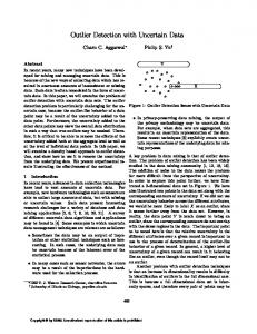
detection values, so they were not included in the stage 2 calculations. Figure 2 shows the ODVs and the data points that were outside of the ODV limits.
3. EXAMPLE
Stage 2 calculates the actual ODVs that are used in determining which data are outliers. For this example, a value of p2 = 0.05 was chosen. Using Equation (4), this resulted in a k value of 4.47. Equations (6a) and (6b) were then used to calculate ODVU and ODVL. The sample mean of the truncated dataset was 7.1 with a standard deviation of 1.9. This resulted in outlier detection values of 15.6 for ODVU and -1.5 for ODVL. Figure 3 shows two data points—20 and 25—were identified as outliers. These calculations assumed a non-unimodal distribution and a The unimodal probability of outliers (p2) of 0.05. distribution calculations will be shown next, using the same example data.
The Chebyshev outlier detection method works when data are integer or continuous. The method is not designed to find outliers within qualitative datasets. An example was created to work through the steps using integers for simplicity. First the calculations will be performed assuming that the data have no distribution (non-unimodal). Then the same process will be performed assuming that the data are unimodal.
ODV(L)
10
ODV(U)
Step 1 Outliers
0
10
Frequency
5
15
Frequency
15
A sample dataset was designed to show how the Chebyshev outlier detection method works. The dataset consists of 50 data points, with the following values and number of the data value shown in parentheses: 0 (1), 5 (4), 6 (10), 7 (16), 8 (12), 9 (3), 10 (1), 15 (1), 20 (1), and 25 (1). Figure 1 shows a histogram of these data. Outliers will be determined using both the non-unimodal method and unimodal method for example and comparison purposes.
-5
0
5
10
15
20
25
5
Data Value
0
Figure 2 – Non-Unimodal Stage 1 Outliers Identified 0
5
10
15
20
25
Data Value
Unimodal Chebyshev Outlier Method Example As can be seen in the histogram in Figure 1, the data appear to be unimodal because it contains only one peak. This indicates that the unimodal Chebyshev outlier method is appropriate to use. This subsection will identify outliers using the unimodal method, and then the results can be compared to the results just discussed using the nonunimodal method.
Figure 1 – Histogram of the Sample Data Non-Unimodal Chebyshev Outlier Method Example Although the data appear to be unimodal, this subsection will assume the data are not unimodal for illustrational purposes. The first step is to find which data points are possible outliers that should not be included in calculations of the mean and standard deviation. Both upper and lower tails will be explored. A value of p1 = 0.10 was chosen. Using Equation (4), this resulted in a k value of 3.16.
The first stage is to find which data points are possible outliers that should not be included in calculations of the mean and standard deviation. A value of p1 = 0.10 was chosen, and both tails will be explored. Using Equation (5) resulted in a k value of 2.11.
The next part within stage 1 is to calculate ODV1U and ODV1L. Equations (6a) and (6b) were used to make these calculations. The sample mean of 7.7 was used to estimate µ, while the sample standard deviation of 3.6 was used to estimate σ . This resulted in ODV1U = 19.13 and ODV1L = 3.73. Two data points (20 and 25) were outside the 4
10
15
= 2.43. Four data points (0, 15, 20, and 25) were outside the detection values. These data points were considered to be outliers. Figure 5 shows the ODV values and the outlier data points that were outside the ODV limits.
ODV(U)
15
ODV(L)
ODV(U)
0
Outliers
5
10
15
20
25
5
0
10
Frequency
5
Frequency
ODV(L)
Data Value
0
Figure 3 – Outliers Identified Using Non-Unimodal Chebyshev
0
15
20
25
Comparison of the Methods Both methods used the same data and the same probabilities of outliers with p1 = 0.10 and p2 = 0.05. In comparison, the non-unimodal Chebyshev outlier method identified two outlier data points, 20 and 25. The unimodal Chebyshev outlier method identified four outlier data points—0, 15, 20, and 25. The unimodal method will always result in tighter limits. It is recommended that if the data are expected to be unimodal, the unimodal Chebyshev method be employed.
ODV(U)
The decision as to what the probability values should be is a key to the outlier decision making process. The researcher needs to assess the risk and cost involved in making the error of identifying an outlier incorrectly and the error in not identifying a data point that is an outlier. If it is more costly to incorrectly identify a data point as an outlier, then the probabilities should be set very low. If the incorrect identification of data points as outliers is low cost and low risk, then the probabilities should be set higher.
10
15
10
Figure 5 – Outliers Identified Using Unimodal Chebyshev
5
Frequency
5
Data Value
The next step within stage 1 is to calculate ODV1U and ODV1L. Equations (7a) and (7b) were used to make these calculations. The mode (M) was 7 for the sample data. B was calculated as 3.68 from Equation (3) using the sample standard deviation of 3.6 (σ), and the sample mean of 7.7 (µ). This resulted in ODV1U = 14.76 and ODV1L = -0.76. Three data points (15, 20, and 25) were outside the detection values, so they were not included in the truncated dataset used in the stage 2 calculations. Figure 4 shows the ODVs and the data points that were outside the ODV limits.
ODV(L)
Outliers
Outlier
0
Step 1 Outliers
0
5
10
15
20
25
4. CONCLUSIONS
Data Value
Data outliers can have a significant impact upon data-driven decisions. In many cases, the outliers do not reflect the true nature of the data and, hence, should not be included in the analyses. The outlier detection method discussed in this paper uses Chebyshev’s inequality to form a data-driven outlier detection method that is not dependent upon knowing the distribution of the data. It also does not rely on domain knowledge to determine outliers.
Figure 4 – Unimodal Stage 1 Outliers Identified Stage 2 calculates the actual ODVs that are used in determining which data are outliers. For this example, a value of p2 = 0.05 was chosen. Using Equation (5), this resulted in a k value of 2.98. Equations (7a) and (7b) were then used to calculate ODVU and ODVL. The mode (M) was 7 for the sample data. B was calculated as 1.53 from Equation (3) using the sample standard deviation of 1.53 (σ) and the sample mean of 6.9 (µ), both calculated from the truncated dataset. This resulted in ODVU = 11.57 and ODVL 5
Scott Cooley is a Research Scientist at Battelle–Pacific Northwest Division. He has applied statistical methods such as optimal experimental design formulation and development of regression models (particularly mixture models) to the problems of nuclear waste immobilization (vitrification). He also has used multivariate statistical methods such as principal component analysis and cluster analysis in a variety of applications to aviation safety. Mr. Cooley has experience with several prominent statistical and computational software packages. He has a BS in mathematics from BYU-Hawaii, an MS in mathematics from the University of Idaho, and an MS in statistics from Montana State University.
ACKNOWLEDGMENTS Several people made major contributions to this effort. Irv Statler, Linda Connell, and Mary Connors of NASA Ames and Loren Rosenthal of Battelle–Mountain View envisioned the overall nature of the program and arranged for funding as part of the NASA Aviation Safety Modeling and Monitoring program over the last several years.
REFERENCES [1] Bernard Ostle and Linda C. Malone. Statistics in Research. Ames, Iowa: Iowa State University Press, 1988.
BIOGRAPHIES Brett Amidan is a Senior Research Scientist at Battelle– Pacific Northwest Division. He has been working in the Aviation Performance Measurement System (APMS) program for NASA Ames for over six years. He has developed and led development of mathematical algorithms applied within the APMS program. He also performs multivariate analysis, experimental design, and simulation efforts on a variety of other projects at Pacific Northwest National Laboratory operated for the U.S. Department of Energy by Battelle. He previously served as Statistics Coordinator at Clinical Research Associates where his main focus was in experimental design. He has an M.S. in statistics from Brigham Young University. Dr. Thomas Ferryman is a Battelle Chief Scientist with more than 30 years of experience in system engineering and mathematics/statistics. He leads the technical development of aviation safety data analysis tools (numeric, categorical and/or text data) for NASA. He also has developed prognostic tools for use on gas turbine engines. Prior to coming to Battelle, Dr. Ferryman was Chief Systems Engineer for Lockheed leading a major weapon system modification (AC-130H Gunship).
6