Decentralized Model Order Reduction of Linear Networks ... - CiteSeerX

24.2

DeMOR: Decentralized Model Order Reduction of Linear ∗ Networks with Massive Ports Boyuan Yan† , Lingfei Zhou† , Sheldon X.-D. Tan† , Jie Chen† and Bruce McGaughy‡ †

Department of Electrical Engineering, University of California, Riverside, CA 92521 ‡ Cadence Design Systems Inc., San Jose, CA 95134

ABSTRACT

a good approximation of the input-output behavior. Existing approaches may generally be divided into two broad categories: the moment matching based methods and the balanced truncation based methods. In the former case, the system is projected onto the Krylov subspace to match dominant moments while in the latter case the system is projected onto a subspace, which is both easily controllable and easily observable. Moment-matching based methods have been a great success owning to their efficiency. These methods perform implicit moment-matching by projecting the original system onto a Krylov subspace, and in this process, stability, passivity and structure information inherent to RLC circuits can be preserved by exploiting the internal structure of the RLC formulation [3, 14, 9, 12, 15]. While suitable for reduction of large-scale circuits, moment-matching based techniques do not necessarily generate models as compact as desired. Nevertheless, another approach, the truncated balanced realization (TBR), which has been well developed in the controls community [8], can be employed to advantage. Recently, algorithms [10] were presented to compute guaranteed passive reduced models of controllable accuracy, which pose no constrains on the internal structure of state-space description of the model. Unfortunately, the efficiency of model order reduction degrades as the number of ports increases. The reason for the degradation is fundamental and does not depend on any particular reduction algorithm [4]. For Krylov-subspace based algorithms, the cost associated with model computation is directly proportional to the number of inputs, i.e. to the number of columns in the transfer function matrix. For example, in the PRIMA algorithm [9], if only two (block) moments are to be matched at each port, and the network has 1000 ports, the resulting reduced model will have 2000 states. Similarly, in the TBR algorithm, for systems with many inputs, many states may be needed because of the high dimension of the controllable subspace. There has been significant effort devoted to mitigating this difficulty recently, which has led to two classes of approaches. The first class takes advantage of the information of input signal. An extended Krylov subspace (EKS) method was proposed [16], which constructs a transformation matrix based on the dynamics of the circuit as well as the source excitations. More recently, an approximated truncated balanced realizations (TBR) procedure was proposed [13, 11] to obtain compact reduced models by exploiting the correlation information of input signals. The extended TBR (ETBR) method, which considers the input signals similar to EKS, has been proposed in [5]. However, since the modeling process depends on the input signal, once the pattern of input signal has been changed, the model needs to be rebuilt. More important, they become less useful when input information is unavailable a priori. The second type of approaches [2, 4, 7, 6] are based on the SVD of matrix-valued transfer function and attempt to perform both terminal reduction and model order reduction. The pioneering works are SVDMOR/RecMOR meth-

Model order reduction is an efficient technique to reduce the system complexity while producing a good approximation of the input-output behavior. However, the efficiency of reduction degrades as the number of ports increases, which remains a long-standing problem. The reason for the degradation is that existing approaches are based on a centralized framework, where each input-output pair is implicitly assumed to be equally interacted and the matrix-valued transfer function has to be assumed to be fully populated. In this paper, a decentralized model order reduction scheme is proposed, where a multi-input multi-output (MIMO) system is decoupled into a number of subsystems and each subsystem corresponds to one output and several dominant inputs. The decoupling process is based on the relative gain array (RGA), which measures the degree of interaction of each input-output pair. Our experimental results on a number of interconnect circuits show that most of the inputoutput interactions are usually insignificant, which can lead to extremely compact models even for systems with massive ports. The reduction scheme is very amenable for parallel computing as each decoupled subsystem can be reduced independently.

Categories and Subject Descriptors I.6.5 [Simulation and Modeling]: Model Development— modeling methodologies

General Terms Algorithms

Keywords Model order reduction, decentralized, multi-port networks

1.

INTRODUCTION

Model order reduction (MOR) is an efficient technique to reduce the interconnect circuit complexity while producing ∗This work is supported in part by NSF under grant No. CCF-0448534, UC Micro Program #06-252 and #07-105 via Cadence Design System Inc.

Permission to make digital or hard copies of all or part of this work for personal or classroom use is granted without fee provided that copies are not made or distributed for profit or commercial advantage and that copies bear this notice and the full citation on the first page. To copy otherwise, to republish, to post on servers or to redistribute to lists, requires prior specific permission and/or a fee. DAC 2008 June 8-13, 2008, Anaheim, California, USA Copyright 2008 ACM 978-1-60558-115-6/08/0006 ...$5.00.

409

matrices V and W are constructed so that their columns span a Krylov subspace. For example, a typical implementation (PRIMA) is to construct V = W by using the Arnoldi algorithm, thereby spanning a Krylov subspace with A = (G + s0 C)−1 C, R = (G + s0 C)−1 B. Because of the momentmatching properties of Krylov-subspace, the reduced trans˜ fer function H(s) will agree with the original H(s) up to the first m derivatives on an expansion around some chosen point in the complex plane (usually s0 = 0)

ods [2, 4], which exploit the fact that the matrix transfer function may be numerically low rank. Furthermore, the method [7] introduces clustering-based terminal grouping based on more high order moments. More recently, McPack [6] was proposed to combine the tangential interpolation and the SVD framework. However, those approaches still assume that all the input-output pairs are equally relevant. Therefore, a matrix-valued transfer function has to be fully populated. As a result, it is hard to obtain a compact model. In this paper, we propose a decentralized model order reduction scheme where a whole MIMO circuit is decoupled into a number of MISO circuits based on the input-output interactions and each circuit is reduced individually. The decoupling process is guided using the relative gain array (RGA) [1], which measures the degree of interaction of each input-output pair. Our method is based on the observation that for an output terminal, not all the input terminals are relevant, and this relevance is determined by their relative gains. As a result, an MIMO system can be naturally partitioned into many MISO systems and the traditional passivity-preserving model order reduction can be performed on these MISO systems. The new reduction algorithm, termed DeMOR, can perform very efficient reduction on MIMO systems. This paper is organized as follows: In Section 2, we review the relevant model order reduction methods. In Section 3, we introduce the concept of relative gain array. Our new approach DeMOR is described in Section 4. Experimental results are reported in Section 5 to demonstrate the effectiveness of our proposed method. Section 6 concludes the paper.

˜ H(s) = H(s) + O((s − s0 )m )

2.3 SVDMOR The SVDMOR/RecMOR methods [2, 4] were first proposed to explicitly reduce the terminals in the projectionbased reduction framework. For many practical circuits, the input-output correspondence at various ports may be highly correlated. In this case, the input-output matrices can be approximated using low-rank matrices. Applying the standard SVD to the system transfer function at DC gives HDC = LT G−1 B = U ΣV T

B ≈ bk VkT

REVIEW OF CENTRALIZED REDUCTION METHODS 2.1 Projection-based reduction framework

n×k

˜ x(t) + Bu(t) ˜ −G˜ T ˜ L x ˜(t)

(1)

(2)

3. MEASUREMENT OF INTERACTION 3.1 Ideal decentralized systems

A p×p linear time invariant (LTI) system can be described by the following model y(s) = H(s)u(s)

(9)

where u(s) and y(s) are p-dimensional vectors of inputs and outputs, respectively, and H(s) is a matrix of transfer functions. If the transfer matrix is diagonal, 3 2 0 ... 0 h11 (s) 7 6 0 0 h22 (s) . . . (10) H(s) = 4 · · · ··· ··· 5 0 0 . . . hpp (s)

(3)

Often the transfer functions H(s) = LT (sC + G)−1 B ˜ ˜ + G) ˜ −1 B ˜ ˜ T (sC H(s) =L

(8)

Since Hk (s) ≈ lkT (sC+G)−1 bk represents a terminal-reduced MIMO network with k(k < p) ports, it can be easily reduced by any existing method. SVDMOR is still based on a centralized framework and it works well for low rank matrix transfer function. However, a complete matrix-valued transfer function is rarely low rank. In fact, one observation we have is that many input-output interactions are magnitude-wise insignificant, which means a decentralized modeling scheme will be more efficient.

˜ L, ˜ ∈ Rr×p . Order r is much smaller ˜ G ˜ ∈ Rr×r , B, where C, than the original order n, i.e. r  n, but the output y(t) and y˜(t) are approximately equal for inputs u(t) of interest. This can be achieved by constructing matrices W and V whose columns span a useful subspace, and projecting the original equations in the column spaces of W and V ˜ = W T CV, G ˜ = W T GV, B ˜ = W T B, L ˜ = V TL C

(7)

n×k

H(s) ≈ Uk lkT (sC + G)−1 bk VkT

where C, G ∈ Rn×n , B, L ∈ Rn×p , and in which x(t) is the state vector, and u(t) and y(t) represent the input and output, respectively. Typically, we have p  n. Model reduction algorithms seek to produce a smaller system C˜ x ˜˙ (t) = y˜(t) =

L ≈ lk UkT

and lk ∈ R . Now the original circuit where bk ∈ R transfer function is approximately as

An RLC interconnect circuit can be formulated as the following state-space form using modified nodal analysis (MNA) −Gx(t) + Bu(t) LT x(t)

(6)

where U and V are the left and right singular vectors. If there exists a strong correlation between the responses at different input-output ports, the transfer matrix can be well approximated based on k(k < p) dominant left and right singular vectors Uk and Vk . These singular vectors are used to find rank-k approximation for L and B

2.

C x(t) ˙ = y(t) =

(5)

To make V = W , passivity can also be preserved if original system is in the MNA form with L = B.

(4)

˜ are used as a metric for approximation: if H(s)−H(s) ≤
, in some appropriate norm, for some given allowable error
and allowed domain of the complex frequency variable s, the reduced model is accepted as accurate.

then no interaction exists and the system is decoupled into p independent subsystems. In this case, an independent (decentralized) control design can be made in terms of each input-output pair. But practical systems are rarely in the ideal decentralized form. However, it is rare that each output equally interacts with all inputs. As a result, we need to measure how strong the interaction will be for each inputoutput pair.

2.2 Krylov subspace methods

The Krylov subspace Km (A, R) generated by a matrix A and matrix R, of order m, is the space spanned by the set of vectors (R, AR, A2 R, . . . , Am−1 R). Usually projection

410

defines the relative gain between the output y1 and input u1 . Similarly, we have

3.2 Relative gain array (RGA) Relative Gain Array (RGA) is a matrix of interaction measures for all possible single-input single-output (SISO) pairings in an MIMO LTI system [1]. This concept has found widespread utility in process control, and as a system robustness measure. The RGA thus indicates the preferable variable pairings in a decentralized control system based on interaction considerations. We use the following 2 × 2 system with transfer function H(s) to illustrate the concept of RGA » – h (s) h (s) H(s) = h11 (s) h12 (s) (11) 21

λ12 = λ21 = λ22 =

G 11

G 21

G 22

y2

Figure 1: A coupled 2 × 2 system.

function hij . First, assume that u2 remains constant, a step change in input u1 of magnitude u1 will produce a change y1 in output y1 . Thus, the gain between u1 and y1 when u2 is kept constant is given by

g11 |u2 =

y1 | u1 u2

(12)

y1 | u1 y2

λij =

g11 |u2 g11 |y2

g21 |u g21 |y

2

1

g22 |u g22 |y

1

1

= =

(
u1 )|u

1 2
y 2 1
y (
u2 )|u 2 1
y (
u2 )|y 1 1
y (
u2 )|u 1 2
y (
u2 )|y 1 2

(
u2 )|y

(15)

gij |u (yi /uj ) |u = gij |y (yi /uj ) |y

(18) Pp

The sum of all elements in the each column is unity ( i=1 λij = 1, j = 1, 2,P..., p) and the sum of all elements in the each row is unity ( pj=1 λij = 1, i = 1, 2, ..., p). The steady-state relative gain array of the system H(s) can be computed using the following method:

(13)

This can be viewed as a closed loop gain with respect to other terminals. Although the above gains are between the same pair of variables, they may have different values because they have been obtained under different conditions. If interaction exists, then the change in y1 due to a change in u1 for the two cases (when u1 and when y1 are kept constant), will be different. The ratio,

λ11 =

2


y

=

and the relative gains between an output yi and an input uj are given by

This can be viewed as an open loop gain with respect to other terminals. Second, when keeping the output y2 constant, a step change in input u1 of magnitude u1 will result in another change in y1 . In this process, y2 will be affected due to cross-coupling. In order to keep it constant, we need to adjust u2 correspondingly, which will also contribute to the change in y1 . The gain under this new set of conditions is denoted by g11 |y2 =

1

If λ11 = 0, then a change in u1 does not influence y1 and therefore u1 should not be used to control y1 , i.e, u1 is not relevant for y1 . If λ11 = 1, y1 is only influenced by u1 . Intuitively, in the closed loop mode, a change in u1 will cause y2 to change due to couplings and u2 will change as well as y2 needs to be kept constant. But the change in u2 does not affect y1 eventually as the two gains are the same. Therefore, there is no coupling either from u1 to y2 or from u2 to y1 . If 0 < λ11 < 1, this means that the closed loop gain is larger than the open loop gain. The closed loop gain consists of the direct gain from u1 to y1 and the gain through the controlled parts (which is from u2 to y1 ). This implies that u2 also has impacts on y1 . In fact, the change in y1 due to a change in u1 will be increased by the interaction from the other loop. The more λ11 is close to 0, the more impacts there are from u2 . If λ11 > 1, this means that the closed loop gain is smaller than the open loop gain. The change in y1 due to a change in u1 will be held back by the interaction from the other loop. The larger the relative gain is above unity, the larger will be this effect. In this case, the more λ111 is close to 0, the more impacts there are from u2 . If λ11 < 0, the interaction from u2 will take output y1 in a direction away from that u1 is trying to achieve. Also, the more |λ11 | is close to 0, the more impacts there are from u2 . For a general system H(s) with p inputs and p outputs, there will be p × p relative gain elements 2 λ λ12 . . . λ1p 3 11 λ λ . . . λ2p 5 21 Λ = 4 · · · · ·22· (17) ··· λp1 λp2 . . . λpp

y1

G 12

u2

g12 |y

The relative gain array for the 2 × 2 system can be constructed as follows h i λ λ Λ = λ11 λ12 (16) 21 22

22

As shown in Fig. 1, gij is the gain of the respective transfer

u1

g12 |u

Λ(H) = H(0)◦H(0)−T

(19)

where ◦ denotes element-by-element multiplication (often called the Hadamard or Schur product), and H −T is the transpose of H −1 . Note that, although the relative array is typically evaluated at zero frequency, it can be evaluated at any other frequency point. In this paper, since we only use RGA as a measure for interaction and do not need to design a controller, the problem can be simplified. By taking the absolute value of each RGA element and taking the inverse for those larger than

(14)

411

Fig. 2) as

1, the scaled elements will fall into the range of [0, 1]: λij = |λij |(|λij | ≤ 1) λij = |λ1ij | (|λij | > 1)

H1 (s) = bT1 (sC + G)−1 [ b1 H2 (s) = bT2 (sC + G)−1 [ b2 H3 (s) = bT3 (sC + G)−1 [ b3 H4 (s) = bT4 (sC + G)−1 [ b3 H5 (s) = bT5 (sC + G)−1 b5

(20)

For a given output i, if jth input has little effect on ith output, then the scaled RGA value λij ≈ 0

(21)

u1

Therefore, a threshold
, can be set to select dominant inputs. After ignoring all the irrelevant inputs in the i th row (λij <
), we will end up with a decentralized subsystem in terms of the ith output.

4.

y1

THE NEW ALGORITHM: DEMOR

y2

u2

b2 ] b3 ] b5 ] b4 b5 ]

u3

u4

(27)

u5

H1

H2

4.1 Decentralized modeling scheme For the RLC circuit in (1), the transfer function is y3

H(s) = B T (Cs + G)−1 B and the steady-state gain H(0) is the DC gain HDC

y4 H4

HDC = B T G−1 B

(23)

The RGA can be computed as

y5 H5

Λ(H) = HDC ◦HDC −T

(24) Figure 2: A decentralized 5 × 5 system.

In this paper, we select DC to compute the RGA as DC has most of the energy. In fact, we can choose any other frequency point and we have to do that if G is singular, which is similar to the choice of frequency expansion points in Krylov subspace methods. Note that we have to compute the inverse of p × p matrix HDC . However, since p  n, such inversion can still be afforded. If there are p outputs B T = [b1 , b2 , . . . , bp ]T , the model can be decentralized into p models and each corresponds to one output H1 (s) = bT1 (sC + G)−1 B1 H2 (s) = bT2 (sC + G)−1 B2 ... Hi (s) = bTi (sC + G)−1 Bi ... Hp (s) = bTp (sC + G)−1 Bp

In the above explicit framework, insignificant signal transfers are totally ignored. However, if the electrical distances among ports are not long enough, those insignificant inputs, although very little individually, could not be ignored when adding up together. So, in practical, an implicit framework is used, where systems are projected onto the Krylov subspace corresponding to the moments of dominant inputs only but insignificant signal transfers are still coarsely preserved. For the ith decentralized model, the projection matrices Vi is constructed so that the columns span a Krylov subspace Km (A, Ri ), where A = (G + sC)−1 C, Ri = (G + sC)−1 Bi . Note that Bi is composed of the dominant inputs corresponding to the ith output. The ith reduced model is obtained by

(25)

˜ i = ViT GVi , B ˜i = ViT B, L ˜ i = ViT L C˜i = ViT CVi , G

We remark that the decoupling process is not unique here. In fact, we can group several outputs into one sub-model if they share similar dominant inputs. For the ith model, the input matrix Bi is composed of the dominant inputs corresponding to the ith output, which can be determined from the RGA matrix Λ(H). For RLC circuits, if the ith input is the current (voltage) source, then the ith output is the corresponding voltage (current) response at the same port. Therefore, ith output should be dominantly interacted with ith input. A 5 × 5 system is given as follows 2

bT1 6 bT2 6 H(s) = 6 bT3 4 T b4 bT5

b2

b3

b4

b5 ]

(28)

˜ i ≥ 0, and ˜i ≥ 0, G For each reduced model, we have C Li = Bi . As a result, the passivity can be preserved. Note that, for ith reduced model, only the ith output (the output corresponding to the ith row of the output matrix LTi ) is valid. The DeMOR algorithm is shown in Fig. 3.

4.2 Computation cost and parallel computing

For an RLC circuit of order n and with p ports, it will take O(n1.5 ) to compute the DC moment HDC as matrix G is very sparse in general. Then it takes about O(p3 ) to invert HDC . Assume that p  n as this is the typical case, the reduction process is still dominated by O(n1.5 ). After the decoupling process, we need to perform reductions on p subsystems. Each of this system will take about O(n1.5 + rn) to reduce using Krylov subspace method where r is the reduced order. Since those subsystems are not coupled, they can be reduced in parallel in the multi-CPU or network of workstations system, which is very amenable for today’s multi-core computing platforms. If the original system has p ports, then a reduced system of order mp is needed for PRIMA to match m block moments.

3 7 7 −1 7 (sC + G) [ b1 5

H3

(22)

(26)

If we assume output 1 is dominantly interacted with input 1 and 2, output 2 is with input 2 and 3, output 3 is with input 3 and 5, output 4 is with input 3, 4, 5, and output 5 is with input 5, the system can be decentralized (shown in

412

Algorithm: DeMOR Input: H : (G, C, B) ˜ i : (G ˜i, C ˜i , B ˜ i )(i = 1, . . . , p) Output: H 1

1. Solve GM = B for M0

0.8

2. Compute HDC = B T M0

0.6

3. Compute relative gain array Λ(H) = HDC ◦HDC −T

0.4

4. Scale the RGA values to the range of [0, 1]

0.2

5. Set the threshold


0 40 30

6. For output i (i = 1, . . . , p) 7. 8.

40 30

20

20

10

Determine the corresponding dominant input matrix Bi

10 0

0

˜i Model order reduction using PRIMA to obtain H ˜i = V T CVi , G ˜ i = V T GVi , B ˜i = V T B C i i i

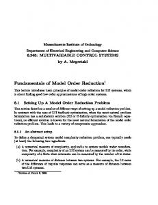
Figure 4: Degree of interactions.

where colspan(Vi ) = Km ((G + sC)−1 C, (G + sC)−1 Bi )

formances of PRIMA, SVDMOR and DeMOR are compared in Fig. 6. In the context of electrical circuits, the fast decaying of interaction can be explained from the concept of electrical distance. For a large-scale network, the voltage response at one particular node is only dominated by the excitations at a small number of ports, which are electrically close to this node. Due to the energy dissipation, those electrically distant ports have little effect and thus can be reasonably ignored. In fact, if the ratio n/p is large, then most likely each output is only dominated by a small number of inputs. So, the larger the number of ports, the more powerful the proposed DeMOR algorithm. We use a power grid network with 10000 nodes and 100 current sources to illustrate this point. Each current source generates a series of pulses of unit magnitude. In this example, the output is dominately interacted with 8 inputs, whose RGA values are above the threshold 0.1, as shown in Fig. 7. The DeMOR reduced model of order 24 is accurate enough while the PRIMA reduced model of order 200 can not achieve the same performance as shown in Fig. 7.

Figure 3: The DeMOR algorithm. The cost of solving the reduced system is O(m3 p3 ) as the reduced system is a full matrix. On the other hand, if we decentralize the original system into p submodels (in the worst case that one submodel corresponds to one output), we assume each submodel has p˜ dominant inputs (˜ p