terference sources on WiFi traffic using commodity WiFi hardware alone. ... non-WiFi interference in ways that have not been possible before. ...... 5 Conclusion.
Catching Whales and Minnows using WiFiNet: Deconstructing Non-WiFi Interference using WiFi Hardware Shravan Rayanchu, Ashish Patro, Suman Banerjee University of Wisconsin Madison Abstract
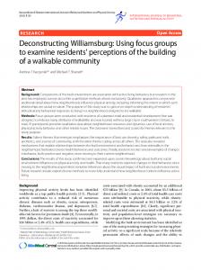
(Interference estimation + Localization) WiFiNet Controller
We present WiFiNet— a system to detect, localize, and quantify the interference impact of various non-WiFi interference sources on WiFi traffic using commodity WiFi hardware alone. While there are numerous specialized solutions today that can detect the presence of non-WiFi devices in the unlicensed spectrum, the unique aspects of WiFiNet are four-fold: First, WiFiNet quantifies the actual interference impact of each non-WiFi device on specific WLAN traffic in real-time, which can vary from being a whale — a device that currently causes a significant reduction in WiFi throughput — to being a minnow — a device that currently has minimal impact. WiFiNet continuously monitors changes in a device’s impact that depend on many spatio-temporal factors. Second, it can accurately discern an individual device’s impact in presence of multiple and simultaneously operating non-WiFi devices, even if the devices are of the exact same type. Third, it can pin-point the location of these non-WiFi interference sources in the physical space. Finally, and most importantly, WiFiNet meets all these objectives not by using sophisticated and high resolution spectrum sensors, but by using emerging off-the-shelf WiFi cards that provide coarse-grained energy samples per sub-carrier. Our deployment and evaluation of WiFiNet demonstrates its high accuracy — interference estimates are within ±10% of the ground truth and the median localization error is ≤ 4 meters. We believe a system such as WiFiNet can empower existing WiFi clients and APs to adapt against non-WiFi interference in ways that have not been possible before.
1
Cordless phone transmissions AP1
WiFi frames
AP3
Client 1 AP2
Microwave oven transmissions
Client 2 Cordless phone (interferer)
Microwave Oven (interferer)
Figure 1: Illustration of WiFiNet’s architecture.
WiFi communication (Figure 1). More specifically, through WiFiNet we can answer the following questions — how much interference is any non-WiFi RF transmitter (e.g., a Bluetooth headset, an active analog phone, or a microwave oven) causing to an existing WiFi communication and where in the physical space is each such non-WiFi interferer located? Much of the prior work has employed custom hardware to tackle non-WiFi interference. Examples include commercial products such as AirMaestro [1] and Wispy [4] that build specific signatures to detect the presence of a device. Recent research efforts (e.g., RFDump [13], DOF [8], TIMO [18]) have used the flexibility allowed by software radios to develop novel signal processing techniques and physical layer designs to co-exist with these devices. The unique aspect of WiFiNet is that it is built entirely on top of standard WiFi network interface cards (NICs). In particular, an emerging class of WiFi NICs, such as those based on the Atheros 9280 chipset, as part of their WiFi frame decoding process, provide coarsegrained energy samples per sub-carrier of a WiFi channel. These energy samples are a few orders of magnitude lower in resolution than those available to sophisticated spectrum analysis tools. In our recent work Airshark [16], we have shown that even with such a low resolution system, a regular WiFi node (either an Access Point or a client) can individually detect the presence of non-WiFi devices. Airshark is, however, is only the first step in the broad space of deconstructing non-WiFi interference and quantifying their impact on WiFi links. WiFiNet leverages collaboration between multiple WiFi nodes to address both quantification of interference impact and localization of these interferers, as we explain below. Quantifying non-WiFi interference impact in realtime: The mere presence of a non-WiFi device, as detected by Airshark, in the vicinity of a WiFi transmitter is not always harmful. For instance, an active analog
Introduction
WiFi devices share the unlicensed spectrum with a plethora of other devices and technologies. A few examples include Bluetooth headsets, ZigBee devices, cordless phones, various game controllers (Xbox, Wii, etc.), and custom wireless security camera systems. Even non-communicating appliances such as microwave ovens, leak energy into this spectrum. Each such device can cause interference to WiFi communication. Since WiFi’s underlying standard (IEEE 802.11) does not have any explicit mechanism to recognize such non-WiFi sources of interference, typical WiFi links have no reasonable way to guard against such interference. In this paper, we design WiFiNet — a collaborative neighborhood of WiFi nodes — to “catch” various non-WiFi transmitters causing harmful interference to 1
cordless phone at a specific location, may only have a minimal impact on a particular WiFi link. We call such a low-impact non-WiFi device, a minnow. On the other hand, a microwave oven radiating a significant amount of energy in its vicinity might cause severe disruption to nearby WiFi links. We call such an interferer, a whale. However, the impact of interference from the same non-WiFi device can quickly change over time. For instance, if the microwave oven’s setting is adjusted to operate with a low power level, this device may suddenly turn into a minnow. On the other hand, if the cordless phone user moves to a different location which is closer to the WiFi link, this device might turn into a whale with respect to this WiFi link. It is even possible that the impact of the cordless phone on the WiFi link changes due to properties of the WiFi link itself. For example, when the WiFi link is operating at 54 Mbps, the disruptive impact of the cordless phone is quite high, with the impact decreasing as a rate adaptation algorithm reduces the WiFi link’s choice of PHY rates. WiFiNet tracks this continuously changing impact of non-WiFi transmitters on WiFi communication in real-time, adjusting its interference estimates immediately as operating parameters change (e.g., the microwave power setting is changed, or the WiFi device’s PHY rate selection algorithm starts operating with a higher rate). Locating non-WiFi interferers: WiFiNet also determines the physical location of such non-WiFi transmitters immediately, so that the precise source of such interference can be determined, and if needed, such interfering devices can either be re-configured or disabled. Through these new and unique capabilities, WiFiNet provides new RF management tools for WiFi environments using off-the-shelf WiFi NICs only, obviating the need for sophisticated wireless hardware. In fact, WiFiNet can be easily implemented and integrated into enterprise WiFi APs to achieve improved mitigation strategies against non-WiFi interference for enterprise environments.
1.1
and employs signal clustering techniques operating on some device specific attributes (when available) and signal strength observations gathered by multiple WiFi detectors to identify the unique transmission contributions from different, potentially identical, non-WiFi devices. Our prior work, Airshark, builds signatures of each device type to detect the presence of any such device in the vicinity of the detecting WiFi node. But such an individual WiFi node is not able to determine if there is only one or two or three different cordless phones in the vicinity, and hence, cannot attribute which part of wireless transmissions belong to which such interferer. How to estimate each device’s impact? After segregating each non-WiFi device’s transmissions, WiFiNet uses fine-grained timing analysis for estimating the impact of each interferer — time-frequency overlaps between the WiFi frames and non-WiFi device’s transmissions are analyzed and correlated with the outcomes (frame success or loss) to discern the impact of each device. Our technique works well for both low and high duty (duty of 100%) devices. In our design, we take into account the carrier sensing interference, interference from WiFi sources and multiple PHY rates of operation used by WiFi links. How do we localize the non-WiFi device? Localization in indoor wireless environments is a well studied problem [5, 6, 20, 23]. Common techniques include signal strength based triangulation [23] and RF fingerprinting approaches [5]. However, the key requirement for such localization approaches is for multiple detectors to detect the same transmission at different signal strengths. In the commonly known WiFi localization techniques, this is easy because the different detectors decode the same wireless frame and use the frame’s identity to ensure sameness. In our case, the WiFi detectors cannot decode the nonWiFi transmissions, and hence cannot immediately assign the same identity to “pulses” received from the nonWiFi transmitters. A core challenge that we needed to solve is for different WiFi detectors to determine which received pulses correspond to a single transmission from the same non-WiFi device. The next challenge is to build a model for localization. Propagation characteristics are similar for both WiFi and non-WiFi transmitters since they operate on the same frequency. WiFiNet exploits this fact and builds the model by exchanging WiFi frames and recording signal strength measurements. Since the transmit power of non-WiFi devices can be arbitrarily different from that of WiFi nodes, the model takes this into account by operating on the difference in received signal strengths. Through experiments, we show the feasibility of this approach for non-WiFi device localization using WiFi-only detectors.
Challenges in designing WiFiNet
In designing and implementing the capabilities of WiFiNet, we had to overcome the following set of challenges: How to detect multiple devices of the same type? In many wireless environments, there are multiple devices of a given type, e.g., two different cordless phones. It is possible that among these two phones, one is a whale and causes 80% loss in throughput to a WiFi link, while the other is a minnow and causes only 5% loss in throughput. To differentiate between these two interferers, WiFiNet needs to determine how many devices of each type are operating at any given instant. To achieve this goal, WiFiNet utilizes tight clock synchronization, 2
3
1
2 Captured WiFi Frames
3 2
5
APs Generic, RSS based clustering
4
Consolidated pulses
Time
Airshark
2
3
NO Consolidation criteria
4
Captured WiFi Frames
4 Per-Device Pulse Trace
1 Captured pulses WiFiNet AP
Airshark
2
1
3 Pulse consolidation (Sec 2.1)
Interferer 1
4
Overlap analysis
Link 1
5 Captured WiFi Frames
Interferer 2
Locations
APs
1 Frame
Link N
synchronization (Sec 2.1) WiFiNet Controller Operations
Unique Devices
5 3
4
1
Device-specific clustering
4 Pulse Clustering (Sec 2.2)
BW resolution WiFiNet AP
Time offset
Prob.
1
YES
RSS
Airshark
Sampling resolution
RSS
WiFiNet AP
(Sec 2.1) 2 Pulse Synchronization
Frequency
Captured pulses
5 Inteference Estimation (Sec 2.3)
Per- Link Frame summaries
6
Device Localization (Sec 2.4)
Interferer 1 (Whale) affects Link 1, at Room 7331 WiFiNet Output Interferer 2 (Minnow) at Room 5388
Figure 2: Flow of operations in WiFiNet. WiFiNet APs capture spectral samples as well as WiFi frames. Each AP runs Airshark [16] to detect non-WiFi devices and output non-WiFi pulses (transmissions) tagged with device type. (1) WiFi frames are used to synchronize the clocks at the APs. (2,3) Synchronized clocks at the APs are then used to consolidate the pulses across multiple APs using a heuristic (§2.1). (4) Consolidated pulses are clustered using RSS and device-specific attributes to output unique non-WiFi device instances and their pulses (§2.2). (5) For each non-WiFi device instance and WiFi link, the interference estimation module analyzes the impact of the device on the link using transmission overlaps (§2.3). (6) Model-based localization algorithms are used to localize each non-WiFi device instance (§2.4).
Summary of key contributions: Summarizing, the key contributions of our WiFiNet system are three-fold: (i) it detects and discerns the transmission contributions of different non-WiFi interferers in the vicinity of the WiFi detectors; (ii) it attributes interference impact of each such non-WiFi device for any given WiFi link, classifying them as whales, minnows, or anything else in between, through collaborative observations; and (iii) it pinpoints the location of each such non-WiFi interferer so that they can be independently re-configured or disabled. All of these capabilities are implemented using WiFi-only detectors. The entire WiFiNet system has been implemented using the Atheros AR 9280 based WiFi NICs, and evaluated in detail through various experiments. Our results indicate a typical impact determination accuracy of > 90% and a localization error of ≤ 4 meters in these environments.
2
captures spectral samples as well as WiFi frames. APs run Airshark [16] to process the spectral samples and perform device detection. Post detection, Airshark outputs a set of “pulses” (time-frequency blocks representing non-WiFi device transmissions). Since WiFi hardware cannot decode non-WiFi pulses, Airshark can only provide limited information for each pulse — pulse’s start and end timestamps, its center frequency and bandwidth, its average received power, and a tag that indicates its device type (e.g., Bluetooth). Next, APs also process the captured WiFi frames to create a per-client frame transmission summary: frame start and end timestamps, PHY rate, and reception status (i.e., whether the AP received an ACK for this frame or not). The proximity between the two radios ensures that the detector radio receives the majority of frames transmitted by the regular radio due to capture effect, thereby creating an accurate summary of frame transmissions [21]. The per-client WiFi frame transmission summaries and the captured non-WiFi pulse traces are forwarded to the controller to identify the individual non-WiFi device instances, estimate their interference impact and localize them. Figure 2 presents the overall control flow. We now explain each of these tasks in detail.
WiFiNet
We start by presenting an overview of WiFiNet’s architecture, followed by the details of its design and operation. Architecture and flow of operations. WiFiNet employs collaborative observations from multiple WiFi-only detectors spread across a network to perform its nonWiFi device interference estimation and localization operations. Since most enterprise APs today come equipped with multiple WiFi radios, one way to deploy WiFiNet would be to employ one of the radios as a detector. In such a setting, WiFiNet can function as follows. All the enterprise APs are connected to a central controller over an Ethernet backplane. Each AP can have two radios: (i) a regular radio used to communicate with the clients, and (ii) a detector radio that continuously
2.1
Identifying unique pulses
Since the same pulse can be received by multiple APs in the WLAN, the first task for the controller is to consolidate the traces and identify the unique pulses transmitted by different non-WiFi devices operating in the environment. To do this, the controller has to identify the “common” pulses received by the APs and create a single consolidated pulse. However, finding common pulses is 3
2.2
signal strength (dBm) signal strength (dBm) signal strength (dBm) signal strength (dBm) signal strength (dBm) signal strength (dBm)
Time (ms) Time (ms) Time (ms) Time (ms) Time (ms) Time (ms)
8 2842 -40 8 2842 -40 Handset 1 Handset 1 -60-40 82842 8862842 2842 -40 2842 -40 2840 8 -60 -40 6 Handset 1 1 Handset 2 2840 Handset Handset 1 Handset 1 -80-60 2 -60 -60 5 ms Handset 6 6 6642840 -80 -60 2840 2840 5 ms 2838 2840 4 2838 Handset Handset Handset 22 2 2 -80 -100 -80 Handset -80-80 5 ms5 ms -100 Base 2 5 ms 5 ms Base 1 42838 2838 4422838 2838 2836 4 Offset 1 Base 1 Base 1 Base 2 -120 2 2836 -100 -100 -100 OffsetOffset 1 Base 2 2 -120 -100 22Base 2 BaseBase Base 1 1 Base 1 Base 22836 2836 2202836 Offset 2 2836 2834 -140 Offset 2 Offset Offset 1 1 11Offset -120 -120 -120 0 -120 2834 -140 Offset Offset 2 2 Offset 22Offset 2834 -140 02834 -140 00 2834 2834 -140 00 -140 10 20 30 40 50 0 10 20 30 40 50 Frequency bins (CF: bin 28, 2452 MHz) 0 10 20 30 40 50 0 10 20 30 40 50 0 10 20 30 40 50 Frequency bin 28, MHz)50 0 bins 10(CF:20 30245240 Frequency binsbins (CF: bin 28, 2452 MHz) Frequency (CF: binbin 28, 2452 MHz) Frequency bins (CF: bin 28, 2452 MHz) Frequency bins (CF: 28, 2452 MHz) Figure 3: Heatmap of 4 FHSS cordless phone devices (2 base/handset pairs) captured by a WiFiNet AP, showing the timing property. Base 1 Handset 2 16.66
10 7.5
Handset 1
5 2.5
Oven 2
15
Base 2
Offset (ms)
Offset (ms)
not straightforward as WiFi APs cannot decode non-WiFi pulses. Pulse consolidation. WiFiNet uses a heuristic to consolidate the pulses: if two APs receive a pulse that has the same device type (e.g., Bluetooth), has the same start and end times, has the same center frequency and bandwidth, then most likely the APs received the same pulse (transmitted by a particular non-WiFi device). In practice, we allow a certain leeway as these parameters might not exactly match e.g., we allow the maximum difference between the pulse start (and end) times to be FFT sampling resolution of the WiFi card (116µs for AR9280 card) and that between pulse center frequencies (and bandwidths) to be resolution bandwidth of the WiFi card (312.5 kHz or equal to 802.11 sub-carrier spacing). To apply the heuristic, however, would require the pulse traces at the APs to be synchronized. How do we synchronize the pulse traces without knowing common pulses (i.e., reference points)? WiFiNet solves this issue by leveraging the WiFi hardware — the timestamps of the pulses are derived from the same clock that is used to timestamp the captured WiFi frames. WiFiNet first synchronizes the clocks at all the APs using captured “common” frames as reference points, and then uses the synchronized APs to find “common” pulses. We implement a graph-based, opportunistic synchronization approach similar to [22]: the controller first synchronizes “pairs of APs” using common reference frames, and then transitively synchronizes all APs. To account for the clock drift, the synchronization process is repeated every 100 ms, which results in tight synchronization between the APs (an error of < 4 µs). Since, this technique is completely passive, it doesn’t generate any additional wireless traffic. Output from consolidation. The controller applies the appropriate synchronization offsets to each AP’s pulse trace and then finds the common pulses among the APs using the heuristic mentioned above. The consolidation process can be carried out efficiently as the pulses are sorted by time. After consolidation, the controller is left with unique pulses transmitted by non-WiFi devices, and for each unique pulse, we associate an RSS vector r = [r0 , . . . , rN −1 ] that represents the received power of this pulse at each of the N APs in the WLAN. We set ri to the average received power of the pulse at ith AP, if the pulse was indeed received this AP, otherwise ri = φ.
-40
10
RSS -60
5
40 80 120 160 Merged pulses Pulses
Handset 2
Base 2
0
0
Base 1
-80
Base 1
0
Handset 1 Base 21 Handset Handset 2
Oven 1
-40
-80
0
500 1K ON periods
-60 RSS
-60 -40
RSS
-80
Figure 4: Segregating pulses in the presence of multiple, simultaneously operating devices of the same type, based on WiFiNet’s device specific and generic clustering. Figure shows clusters of pulses from (left) 2 FHSS cordless phone base/handset pairs (4 FHSS cordless devices) using pulse start time offset (middle) 2 Microwave ovens using ON-period offset (right) 4 FHSS cordless devices using a generic, RSS based k-means + EM-clustering technique using 3 WiFiNet APs.
rithms determine “the number of clusters” (non-WiFi device instances), and assign each pulse to a cluster. The combination of (device type, cluster center) is then used as the ID for this device instance. In our current prototype, we implement (i) a generic, RSS based clustering that is applicable to all non-WiFi devices and (ii) clustering based on timing properties that is specific to some non-WiFi device types. We now explain both approaches. 2.2.1
Generic clustering based on signal strength WiFiNet’s generic clustering approach operates on N dimensional RSS vectors (i.e., vector sizes grow with the number of APs). To improve the performance of clustering algorithms, we use some optimizations: (i) clustering is performed every scan window (5 secs in our current prototype) to keep the number of pulses low, (ii) dimensions corresponding to APs not receiving any pulse in the current window are discarded. Before proceeding with clustering, however, we have to tackle the another problem: some RSS vectors might have missing values (i.e., ri = φ) for some columns. This is because APs might capture pulses intermittently (i) as they are far from the device, or (ii) due to a stronger signal from other WiFi or non-WiFi transmissions [16] that overlapped with the pulse. While it is possible to define a distance function for clustering that ignores missing values in the vectors, such a function is unsuitable for many traditional clustering algorithms as it doesn’t satisfy certain mathematical properties such as the triangle inequality [10]. This presents us with two choices, (i) use clustering algorithms which allow a certain degree of freedom in the formulation of a suitable distance function or (ii) fill in the missing val-
Identifying unique device instances
After obtaining the unique pulses, the next task for the controller is to detect the number of non-WiFi device instances, segregate the pulses belonging to each instance and establish a unique ID for it. WiFiNet first segregates the pulses according to their device type, and employs clustering algorithms for further segregation. The algo4
ues using a best-effort approach, and then use traditional clustering algorithms. We explored both these choices. Clustering algorithms. For approach (i), we explored density-based clustering, dbscan [12] that allowed us to use a distance function that ignores the missing values — distance between two pulses was calculated using a function that operates only on received signal strengths at “common” APs and ignores other APs whose RSS values are missing [19]. For approach (ii), a standard way is to use imputation, where missing values are replaced using “most likely” values. In WiFiNet, we use EMImputation [3], a well known imputation method, where the missing values are replaced by using expectation maximization with a multi-variate normal model. After imputation, we can use traditional clustering mechanisms as the distance function (e.g., Euclidean) can now operate on all the columns of the vectors. We experimented with several clustering algorithms and found that a combination of k-Means and EM-clustering perform the best: we iteratively run the k-Means clustering algorithm with different values of k (1 ≤ k ≤ kmax ), and then pick the best solution [3]. This is used as the initial solution to the EM-clustering algorithm, which outputs the final non-WiFi device instances and the corresponding pulses. In our experiments, we set kmax = 10, i.e., we assume that the maximum number of simultaneously operating devices of the same type to be 10. Figure 4 (right) shows the result for RSS based clustering of 4 FHSS cordless phone devices using 3 WiFiNet APs. In §3, we evaluate both the clustering algorithms. 2.2.2
Time F1
WiFi Link Transmissions Non-WiFi Device Transmissions
F2
T1
synchronized frame summary (e.g., from AP1)
F3
T2
Loss
Success
Loss
synchronized pulse trace (e.g., from AP2) Reception status
Figure 5: Illustration of interference estimation in WiFiNet.
putes the offset for start times of the microwave pulses (ON periods) as t mod 16.66 and uses this to segregate their pulses. Figure 4 (middle) shows the result of clustering pulses from two microwave ovens operating simultaneously. The RSSI based generic clustering doesn’t work very well when the multiple devices of the same type are placed close to each other. The device specific properties (based on timing properties) are not affected by the distance between multiple devices and thus improves clustering performance. But, these device specific properties are not available for all interferer types. Thus, WiFiNet uses both clustering mechanisms to identify the number of unique device instance.
2.3
Interference Estimation
After clustering, the WiFiNet controller has a set of clusters, each representing a unique non-WiFi device instance. We now explain how the controller can analyze the interference impact of each device instance. Intuition and Overview. For each non-WiFi interferer instance and a WiFi link, the WiFiNet controller performs interference analysis by correlating the the link’s frame transmission with the non-WiFi device’s pulse transmissions and observing the reception status of the frames. It measures the impact of a non-WiFi device on a WiFi link by computing the probability of a frame loss when the frame overlaps with a simultaneous transmission from the non-WiFi device. Intuitively, the extent of interference is directly proportional to the probability of losing overlapping frames. For instance, in Figure 5, the controller observes that frames transmitted on a link are unsuccessful whenever a non-WiFi device’s pulse overlaps with the frame in time (and frequency) i.e., frames F1 and F3 overlap with non-WiFi device pulses T1 and T2 , and are lost. It can therefore infer that the device strongly interferes with the link. Such fine-grained timing analysis is possible because APs are tightly synchronized (§2.1) and they use the same clock to timestamp both pulses and the frames. We now explain our interference estimation metrics. Metrics for interference estimation. Formally, the interference estimation metrics used in WiFiNet can be explained as follows. Let I be the event that interference
Clustering based on device specific attributes
We found that some non-WiFi device types exhibit certain specific timing properties that can be exploited to provide better clustering performance compared to the generic RSS based clustering approach. In WiFiNet, we implemented such clustering for two non-WiFi device types: — Pulse start time offset for FHSS cordless phones. WDCT cordless phone sets cycle through frames of 10 ms: each frame consists of two short pulses, one emitted by the base at the beginning of the frame and the other by the handset, occurring after 5 ms (both at the same center frequency). Both base and handset then jump to a different center frequency for the next frame. Figure 3 shows the pulses from two cordless phone sets (i.e., 2 base/handset pairs, a total of 4 unique cordless phone devices) captured by WiFiNet. Figure 4 (left) shows that clustering based on the pulse start time offsets (t mod 10) can segregate the pulses belonging to each device. — ON-period offset for microwave ovens. Microwave ovens emissions exhibit an ON-OFF pattern, typically periodic with a frequency of 60 Hz (frequency of the AC supply line) i.e., a period of 16.66 ms [16]. WiFiNet com5
overlapping non-WiFi interferer. We observed that diversity in the frame transmission times [21] as well as the diversity in transmission times of different non-WiFi devices allows WiFiNet to distinguish the true non-WiFi interferer from the other false non-WiFi interferers (i.e., devices that happened to transmit at the same time as the true interferers). In particular, such a diversity allows WiFiNet to observe further transmissions from false nonWiFi interferers that overlap with the frames but do not lead to a frame loss. In our experience, such a transmission diversity arises due to (i) distinct transmission characteristics of different non-WiFi devices (e.g., frequency hopping devices typically emit short pulses at different center frequencies) and (ii) diversity in the usage times of non-WiFi devices [16], where in a typical enterprise not more than 3−4 devices were found to be simultaneously active.
from a particular non-WiFi device causes a frame transmission to be unsuccessful. Let L be the event of an unsuccessful transmission due to background losses (e.g., due to weak signal) and O denote the event of an overlap between the frame transmission and a simultaneous transmission (e.g., a pulse) from the non-WiFi interferer. — (Metric 1) Impact given overlap. Conditional probability, p[I|O] is used to measure the impact given overlap i.e., probability that a frame is unsuccessful given an overlap with a simultaneous transmission from a non-WiFi device. — (Metric 2) Overall impact. WiFiNet also maintains p[I], the overall impact of a non-WiFi device. Here, p[I] is equal to p[I|O]·p[O] (when there is no overlap, p[I|¬O] is simply 0). That is, p[I] is probability of frame loss due to the overall activity from the non-WiFi device. We note that p[I], the overall impact of the interferer, depends on the probability of overlap p[O], which varies based on the link and interferer transmission patterns. Whereas, p[I|O] is not affected by these transmission patterns i.e., p[I|O] indicates the worst case impact of the interferer on the link, which is observed when p[O]=1 (i.e., when the transmissions of link and the interferer always happen to overlap). Next, we explain how these probabilities are estimated by WiFiNet in real-time. Interference estimation. The controller measures the total number of frames transmitted (n) on the WiFi link of interest, the number of frames that overlapped with the non-WiFi device’s transmissions (no ) and nlo , the number of overlapped frames that were unsuccessful. It then computes p[O], the probability of transmission overlap as no /n. Next, the controller computes p[(I∪L)|O] = nlo /no i.e., the probability of an unsuccessful frame transmission due to either background losses or interference from the non-WiFi device, given an overlap in transmissions. It also computes the probability of frame loss when there is no overlap from the interferer, p[L] as nlno /nno . Here, nno = n−no is the number of frames without overlap and nlno is the number of nno transmissions lost. Since L is independent of O, we have p[L|O] = p[L|¬O] = p[L]. Also, I and L are independent events, and so we have p[(I∪L)|O] = p[I|O]+p[L]−p[I|O]·p[L]. That is, � � p[(I∪L)|O] − p[L] (1) pWiFiNet = p[I|O] = (1 − p[L])
2.3.1
Enhancements to the basic technique
Handling high duty devices operating with other devices. Transmissions from multiple devices that always happen to overlap in time can lead to cases where WiFiNet can make incorrect estimates. For example, WiFiNet may identify a false interferer as a true interferer if the transmissions from the false interferer always happen to overlap with that of a true interferer. In our experiments, we found that such a scenario is unlikely when using pulsed transmitters (e.g., ZigBee devices) or frequency hopping devices (e.g., Bluetooth or FHSS cordless phones) that typically emit short pulses. However, operating high duty devices (e.g., analog cordless phones) that continuously emit energy alongside other low duty interferers will cause their transmissions to always overlap that can lead to incorrect estimates. We use two refinements to the basic approach to correctly identify interference impact of a low duty interferer W operating alongside a high duty device H: (i) when computing p[IH |OH ] for a high duty device, we only consider the frames that do not overlap with a transmission from any other non-WiFi device. The background losses p[L] are computed using packet losses when no interferers are present. (ii) For computing the p[IL |OL ] of low duty interferers operating in the presence of high-duty devices, the background losses (p[L]) are computed using using packet loss information when the low duty interferer is not present. These losses include the link proagation losses as well as the losses due to the high duty devices. For more details, the reader should refer to the technical report [19]. Quantifying impact at different 802.11 rates. The impact of a non-WiFi interferer on a WiFi link also depends on the PHY rate being used by the WiFi transmitter. To account for this, the WiFiNet controller records the overlaps and losses separately for each different PHY rate,
Using p[(I∪L)|O] and p(L), the WiFiNet controller estimates p[I|O]. Following this, the controller also computes the overall interference p[I] as p[I|O]·p[O]. Handling overlaps from multiple non-WiFi interferers. In general, a frame transmission may overlap with multiple simultaneous transmissions from potential nonWiFi interferers. In this case, the WiFiNet controller attributes the frame transmission success or loss to each
6
-20
Observed RSSI (dBm) Modeled RSSI (Mean) +3 Stdev -3 Stdev
-30 -40 -50
PDF
Observed RSSI (dBm)
and computes a separate interference estimate for each rate. This helps quickly the estimate interference impact at each PHY rate when using dynamic bit rate adaptation as opposed to high-overhead bandwidth tests that require controlled experiments at each PHY rate to estimate the same [21]. Handling sender-side interference. Similar to the procedure used for interference analysis, the WiFiNet controller can infer whether a WiFi transmitter is deferring to a non-WiFi device by correlating the WiFi frame transmissions with the non-WiFi pulse transmissions. Two cases of interest arise. Case(a) when the WiFi transmitter is not deferring to the non-WiFi device, the WiFiNet controller will observe several instances where the frame transmission starts while the pulse transmission is in progress. Case(b) When the WiFi transmitter is indeed deferring to the non-WiFi device, the WiFiNet controller will not observe instances where frame transmission starts while the pulse transmission is in progress. However, this condition alone is not enough to infer that the WiFi transmitter is deferring to the non-WiFi device, as it may happen that the WiFi transmitter did not have any packets to send while the pulse transmission was in progress i.e., the WiFi transmitter did not contend for the medium. To identify the deferral instances, we use a heuristic similar to the prior work on carrier sense estimation between WiFi links [15, 21]: the controller identifies the deferring frames as those where the difference between the pulse transmission end time and the frame transmission start time is within a certain threshold δw . Here, δw is the maximum time spent by the WiFi transmitter performing back-off and is set to 28+320 µs (DIFS + Max back-off period for 802.11g). The controller can now compute the fraction ∆cs = nd nd +nnd where nnd is the number of Case (a) instances that indicate non-deferral behavior and nd is the number of Case (b) instances that indicate deferral behavior. If the transmitter is indeed deferring, ∆cs would be close to 1. Whereas, if the transmitter is not deferring to the nonWiFi device, the difference in the pulse and frame start transmission times would be uniformly distributed in the interval [0, δp +δw ], where δp is the duration of the pulse. w That is, we expect ∆cs ≈ δpδ+δ . Typically, δp > δw , w therefore ∆cs is low for cases of non-deferral (e.g., for δp for microwave ovens, cordless phones, and Bluetooth devices is 8 ms, 1.25 ms, and 625 µs respectively). In our experiments, using a threshold of ∆cs > 0.8 was able to correctly identify deferring WiFi transmitters (§3.4.2). Extensions to handle WiFi interference. In general, WiFi links can also experience interference from other WiFi links. We extend our basic approach to measure the overlaps between frame transmissions on a particular WiFi link and the frame transmissions on other WiFi links to compute the probability of frame loss due to
-60 -70 -80 0
5
10
15
20
25
30
35
Distance from source (in meters)
0.35 0.3 0.25 0.2 0.15 0.1 0.05 0
Observed RSSI Modeled RSSI
-64 -62 -60 -58 -56 -54 -52 -50 -48 RSSI (in dBm)
Figure 6: (left) Path loss model created by a WiFiNet APs using WiFi transmissions (right) PDF of actual RSSIs observed at a sample location and the model created using a normal distribution.
hidden interference [21]. In §3.1.4, we experiment with non-WiFi interferers operating alongside hidden terminals and show that WiFiNet is correctly able to identify the true interferer.
2.4
Localizing a non-WiFi device instance
WiFiNet uses a computationally efficient, real-time local-
ization scheme that imposes zero profiling overhead, and physically locates the non-WiFi device instance of unknown transmit power using a modeling based approach. Below, we explain our localization models.
2.4.1 Model-based localization Let ˆ r = [ˆ r0 , . . . , rˆN −1 ] be the mean RSS vector of all the pulses present in the cluster assigned to a non-WiFi device instance. For localization, we only consider the APs with valid received powers (i.e., rˆi 6= φ). We divide the entire region into grids of size 0.25 × 0.25 meters. Let i denote the grid location of APi . Let dij denote the distance between grids i and j. Let P (l|ˆ r) denote the probability of the non-WiFi device being at location l, given that the received power vector is ˆ r. We wish to determine the grid location l such that P (l|ˆ r) is maximized i.e., we want argmaxl P (l|ˆ r). Using Bayes’ theorem, P (l|ˆ r) can be written as P (ˆ r|l).P (l)/P (ˆ r). Assuming all locations are equi-probable, and since P (ˆ r) is constant for all l, we have argmaxl P (l|ˆ r) = argmaxl P (ˆ r|l), QN −1 which can be calculated as argmaxl i=1 P (rˆi |l) (assuming independence [23]). Put another way, the grid location l where the non-WiFi device is most likely present can be computed using, N −1 X argmaxl logP (rˆi |l) (2) i=1
Case of known transmit power (Model-TP). If the nonWiFi device instance is at a grid l, then the expected received power at APi (located at grid i) can be modeled as a normal distribution N (µil , σ 2 ), where σ is the shadowing variable, and µil is the expected mean of the received power that can be modeled as µil = Ro − 10γlog10 dil . Here, γ is the pathloss exponent and Ro is the power received from the non-WiFi device when placed at a distance of 1 meter from an AP (referred to as transmit power). How can we estimate γ for the non-WiFi device? WiFiNet APs derive γ using WiFi frames i.e., each 7
Meters
9
AP3 AP2 AP1
18
36 0
9
actual
36 0.8 0.6
AP0
AP5
0.4
AP6
0.2
AP7
36
27
1 AP4
27
18
1
0
0 1 0.8
9 Meters
0.6
18 predicted
27
0.4 0.2
36
2
3
0
Norm. Probability
0
27
Norm. Probability
18
2.4.2 Alternative localization methods We also implemented several other localization schemes ranging from simple methods such as (i) Strongest-AP, picking the AP with the strongest received power as the device’s location, and (ii) Centroid, picking the centroid of three APs with the strongest received powers, to more sophisticated approaches like (iii) an Iterative approach that performs an exhaustive search over all parameters (γ, σ, Ro , l) to find the grid l with the maximum probability, and (iv) a Fingerprinting approach where we collect fingerprints (RSS vectors) at sample locations and localize the device using an approach similar to [5]. In §3, we compare our model based approaches to all these methods.
Meters
Meters
9
0
Figure 7: (top, left) Deployment 1 comprising 8 APs. (rest of the sub-figures) FHSS cordless phone device is placed at the starred location. Grid probabilities for predicted phone locations after processing 1, 6 and all AP pairs when using Model-UTP algorithm.
3
WiFiNet AP uses the data packets or beacons transmitted by neighboring WiFiNet APs to model the propaga-
Experimental Results
We break our evaluation into four parts: (i) we validate WiFiNet’s non-WiFi device interference estimates across a variety of scenarios, (ii) we evaluate WiFiNet’s accuracy in physically locating the non-WiFi devices, (iii) we emulate a non-WiFi interference prone enterprise WLAN scenario and show WiFiNet’s utility in such a setting and (iv) we benchmark different components of WiFiNet and highlight cases where WiFiNet’s performance could degrade. We start by presenting the details of our implementation. Implementation. We implemented WiFiNet using commodity WiFi APs equipped with Atheros AR9280 wireless cards that are connected to a central controller over the Ethernet. Our implementation consists of few hundred lines of C code and 9800 lines of Python scripts that implement non-WiFi device detection functionality at the APs [16], perform synchronization across multiple APs, and implement clustering algorithms, interference analysis and device localization methods at the controller. Evaluation set up. We experiment with devices in 2.4 GHz spectrum, and our current prototype has been tested with 5 different non-WiFi devices types : (i) high duty devices (analog cordless phones), (ii) fixed-frequency pulsed transmitters (ZigBee devices), (iii, iv) two types of frequency hopping devices (FHSS cordless phones, Bluetooth devices), and (v) broadband interferers (microwave ovens). We run our experiments on two different deployments: (i) Deployment 1 used 8 APs (Figure 7) and (ii) Deployment 2 used 4 APs (Figure 17). We experiment with different non-WiFi device locations, 802.11 rates, channel conditions and traffic patterns: (i) UDP with saturated traffic as well as reduced traffic loads, and (ii) replay of real HTTP/TCP wireless traces (§3.1.5). Unless otherwise stated, we run WiFi links on 802.11 rate to 6 Mbps and use backlogged UDP traffic with a packet size of 1400B. Ground truth. We use an approach similar to bandwidth tests [21, 11] (conventionally used to determine in-
tion loss characteristics (Figure 6) — since both WiFi devices and non-WiFi devices operate on the frequency, the propagation loss characteristics of their transmissions are similar. WiFiNet APs also compute σ 2 , by measuring the variance in the received power values (Figure 6 (right)). Knowing µil , σ and rˆi , the controller can compute P (rˆi |l) using N (µil , σ 2 ). Intuitively, each APi propagates a probability that is maximum around a circle with center at grid i and radius equal to µil . If the transmit power Ro of the device is known, plugging in P (rˆi |l) in Equation 2 and iterating over all the grids and APs, we can compute the grid l with the maximum probability of finding the device. Case of unknown transmit power (Model-UTP). If Ro is not known, we can factor it out by considering each pair of APs: if the non-WiFi device is at a grid l, the expected difference in the mean received powers at APi and APj can be modeled as λ(i, j, l) = µil − µjl = 10γlog10 (djl /dil ), and expected difference in the powers follows a normal distribution with twice the variance: N (λ(i, j, l), 2σ 2 ) [6]. Now, knowing (ˆ ri − rˆj ), we can compute P ((rˆi − rˆj )|l) and we can localize the non-WiFi device by finding X � argmaxl logP (rˆi − rˆj )|l (3) i,j
i.e., each AP pair propagates a probability P ((rˆi − rˆj )|l) on every grid l. The probabilities are high for the grids where the difference in received powers (rˆi −rˆj ) is close to (µil −µjl ). After processing all AP pairs, the algorithm outputs the grid l with the maximum probability. — Example. Figure 7 (top, left) shows a deployment of 8 APs along with the location of an FHSS cordless phone (shown using a star). The rest of the figures show how the grid probabilities indicating the location of the phone change after processing 1, 6 and all possible AP pairs. 8
terference between WiFi links) to determine the ground truth impact of a non-WiFi interferer on a WiFi link: we perform controlled experiments using backlogged traffic on the WiFi link and we (i) measure p[L], the loss rate when the interferer is inactive, and (ii) measure p[I∪L], the loss rate when the interferer is active. We can then measure the ground truth i.e., the actual p[I|O] (§2.3) 1 . For experiments involving multiple devices, we measure the ground truth by activating only one device at a time and measuring its impact on the link. We note that the same ground truth (p[I|O]) is valid when multiple devices are activated simultaneously (the overall impact p[I] may change, but p[I|O] remains the same). WiFiNet, however, computes p[I|O] estimates in presence of multiple, simultaneously active devices and WiFi links using any traffic load. Metrics used. For interference estimation, we compare WiFiNet’s real-time, passive interference estimate of “impact given overlap” (p[I|O]) with that obtained using controlled experiments wherein the device is activated in isolation (ground truth). For localization, we report the difference in the actual and the predicted location of the nonWiFi device (i.e., localization error) in meters.
Analog Phone ZigBee
FHSS Phone Microwave
100 80
0.75 CDF
P(I/O) WiFiNet
ZigBee Analog Phone FHSS Phone Microwave 1 y=x
0.5 0.25
60 40 20
0
0 0
0.2
0.4 0.6 0.8 P(I/O) Actual
1
-0.5
-0.25 0 0.25 Error in P(I/O)
Figure 8: (left) Interference estimates obtained using controlled measurements (ground truth) and WiFiNet on 165 link-interferer scenarios comprising 4 different classes of devices. (right) CDF of error in interferer estimates is within ±0.1 for 95% of the cases.
P(I/O)
0.5 0.25
WiFiNet Actual
CDF
1 0.75
0 Analog FHSS ZigBee Bluetooth Phone Phone
100 80 60 40 20 0
One Two Three Four
-0.5 -0.25 0 0.25 0.5 Error in P(I/O)
Validating Interference Estimates
Figure 9: Accurately identifying impact of each interferer in the presence of multiple non-WiFi devices. (left) example scenario showing WiFiNet is able to identify the strong interferers (analog cordless phone, FHSS phone) and weak interferers (ZigBee and Bluetooth devices) accurately. (right) CDF of error in inteference estimates in the presence of multiple interferers.
3.1.1 Single interferer scenarios Method. We experiment with a total of 165 linkinterferer scenarios comprising 4 non-WiFi devices — a microwave oven, an analog cordless phone, an FHSS cordless phone and a ZigBee transmitter. We activate each device in turn, and place it at different distances to vary the interference on the monitored WiFi link. We compute the ground truth (actual p[I|O]) using controlled experiments that measure the link loss rate when the device is active and that when the device is inactive. Next, we randomly activate and de-activate the non-WiFi device while the WiFi link is active and measure WiFiNet’s real-time estimate. Results. Figure 8 (left) shows that WiFiNet correctly estimates a non-WiFi device’s impact — across all device types and different amounts of interference (ranging from weak to strong), WiFiNet’s estimates lie close to the ground truth (the points lie close to y = x). Figure 8 (right) shows that the overall error in WiFiNet’s estimate is within ±0.1 for more than 95% of the cases for all 4 devices.
domly activate and de-activate them, creating scenarios when these devices are simultaneously active and measure WiFiNet’s interference estimate for each device. For ground truth, we activate only one device at a time and perform controlled measurements. We repeat the experiments for different combinations of devices and locations. Results. Figure 9 (left) shows a particular run which comprised two strong interferers (analog phone and FHSS cordless phone) and two weak interferers (ZigBee and Bluetooth devices). We find that WiFiNet is not only able to accurately identify the strong and weak inteferers, but is also able to discern the exact impact of each of these devices in spite of them being active simultaneously. Figure 9 (right) shows the CDF of error in interference estimates for combinations of 2, 3 and 4 devices across 60 runs. While the overall error slightly increases with increase in the number of devices, the error is within ±0.15 for more than 85% of the cases even when operating 4 devices. The slight increase in error is due to increased overlap in the transmissions from multiple devices. We benchmark the effect of overlapping transmissions in §3.4.4.
3.1
We start by validating WiFiNet’s interference estimates across a variety of scenarios.
3.1.3
3.1.2 Multiple interferers of different types Method. In each run, we choose upto 4 random devices of different types, place them at random locations, ran-
Multiple interferers of the same type
Method. We now evaluate WiFiNet’s performance when simultaneously operating multiple devices of the same type. We use 4 FHSS cordless phone devices — one base/handset pair is placed close to the WiFi link (to cre-
1 Knowing p[O], it is possible to determine p[I|O]. Details of the derivation are presented in our technical report [19].
9
(farther from the link)
WiFiNet Actual Base1 Handset1 Base2 Handset2 (4 simultaneous FHSS cordless phone devices)
Figure 10: WiFiNet’s accuracy in the presence of multiple non-WiFi devices of the same type. Out of 4 FHSS cordless phone devices, 2 are placed close to the link, and 2 are placed farther away.
ZigBee
Figure 11: Estimating the interference impact of a WiFi interferer (hidden terminal) and a non-WiFi interferer (ZigBee device).
ate strong interference), whereas the other pair is placed farther away (to create weak interference). Results. Figure 10 shows that WiFiNet is able to (i) accurately identify all 4 FHSS cordless phone devices using clustering mechanisms (benchmarked in §3.4.3) and (ii) accurately identify strong interferers (base/handset pair placed close to the link) and weak interferers (base/handset pair placed farther away from the link).
0 10 20 30 40 50 60 Time (sec)
0
impact given overlap P[I/O]
10 20 30 40 50 60 Time (sec)
1 0.75 0.5 0.25 0
0.5
1 0.5
WiFiNet Actual
1 Packet size0.75 (Bytes) 0.5 0.5 0.25 0.25 0 P[I/O]
WiFi Interferer
2
actual impact p[I]
P[I/O]
ZigBee
4
1 0.8 0.6 0.4 0.2 0
WiFiNet interference pat0.5 the changing Figure 12:WiFiNet WiFiNet’s ability to track Actual terns for a client Actual that is moving away 0.25 from a ZigBee interferer. (left) 0.25 instantaneous throughput at the client (right) delivery in isolation (i.e., in absence of overlap), impact0 given overlap (p[I|O]) and ac0 200 600 tual impact200 (p[I]) are shown. 600 1000 1400
Actual WiFi Interferer
Delivery in isolation
6
0
WiFiNet AirWiz
WiFiNet AP (transmitter)
P[I/O]
1 0.75 0.5 0.25 0
Weak WiFi Interferer with Strong non-WiFi Interferer
Direction of client movement
P[I/O]
P(I|O)
Strong WiFi Interferer (Hidden Terminal) with Weak non-WiFi Interferer
WiFi client (receiver)
Impact on client
Throughput (Mbps)
ZigBee Interferer
P[I/O]
(closer to the link)
P[I/O]
P[I/O]
1 0.75 0.5 0.25 0
0 6 6
24 48 54 36 1212 24 36 rate (Mbps) PHY DataPHY rateData (Mbps)
06 48
1000 Packet size (Bytes)
12 24 36 54 PHY Data 200 600 1000 1400 rate (Mbps) Packet size (Bytes)
Figure 13: Impact of (i) PHY rate and (ii) packet size on p[I|O] in presence of a ZigBee interferer. For (i), packet size is fixed at 1400 bytes, and for (ii), rate is fixed at 12 Mbps. p[I|O] rises sharply with rate, the change in p[I|O] with packet size is less pronounced.
a slight increase, (ii) the impact given overlap p[I|O], which rapidly drops down from 0.98 to 0.2 as the client moves farther away and (iii) the actual impact p[I], owing to the probability of overlap, drops from 0.3 to 0.12. The decrease in the actual impact closely matches with the increase in throughput confirming WiFiNet’s utility in understanding client performance in dynamic wireless environments. Variable 802.11 rates and packet sizes. We evaluate WiFiNet’s ability to dynamically track the changing interference estimates due to changes in (i) PHY rates and (ii) packet sizes used by the links. For ground truth, we perform controlled experiments at each PHY rate, whereas for WiFiNet we enable dynamic rate adaptation using SampleRate and capture the estimates in real-time. Figure 13 (left) shows that WiFiNet’s estimates derived from rate adaptation closely match the ground truth. Since higher rates require higher SINR to decode a frame successfully, impact of the interferer increases with the increase in rate. Next, we fix the PHY rate (to 12 Mbps) and repeat our experiments for different packet sizes. Figure 13 (right) shows that WiFiNet is correctly able to track the slight increase in the interferer’s impact at larger packet sizes. Replay of wireless traces. We evaluate WiFiNet’s performance using publicly available Sigcomm 2004 traffic traces [17]. We partitioned the trace into heavy, medium, and light periods corresponding to periods with airtime utilization of more than 50%, between 20−50%, and less than 20% respectively, at different times of the conference [21]. The HTTP/TCP sessions are then replayed on WiFi links (using the mechanism described in [7]) in the
3.1.4 Mix of WiFi and non-WiFi interference Method. We evaluate WiFiNet’s accuracy when simultaneously operating a WiFi interferer (hidden terminal) and a non-WiFi interferer (ZigBee device). The interferers are placed at different distances from the monitored WiFi link to create two scenarios: (i) strong WiFi interferer with a weak non-WiFi interferer (ii) weak WiFi interferer with a strong non-WiFi interferer. The WiFi interferer’s traffic follows an http on-off model for with sleep and active times derived from a wireless trace [17], whereas the ZigBee device used a constant bit rate. As before, to measure ground truth, we operate the devices in isolation. Results. Figure 11 shows the results. In case (i), WiFiNet finds that losses are more likely to happen when the monitored link’s frames overlap with WiFi interferer’s frames, whereas in case (ii), the losses show a high correlation when frames overlap with non-WiFi device’s transmissions, resulting in accurate estimates for both cases. 3.1.5 Dynamic interference settings Handling WiFi client mobility. We now evaluate WiFiNet’s ability in updating the interference estimates that reflect the changing impact of a non-WiFi interferer due to client mobility. We use the set up shown in Figure 12 (top) where in a WiFi client is moving away from a ZigBee interferer. In the figure, plot on the left shows the instantaneous throughput at the client increases as it moves away from the interferer. The plot on the right shows WiFiNet’s ability to track (i) delivery in isolation (i.e., in the absence of overlap) that shows 10
1400
WiFiNet Actual
48
54
Heavy Profile
Strong
Med.
Medium Profile
Weak Strong
Algorithm Iterative Model-TP Model-UTP
Light Profile
Med. Weak Strong
Med.
25th %ile. 549 ms
median 972 ms
75th %ile 1.7 sec
1
75th %ile 4m 3m 4m
1
Model-UTP
CDF
0.8
Max error 10m 8m 11m
Model-TP
0.8 Model-UTP
0.6 Model-TP
0.4
0.6 Fingerprint
0.4
Centroid
Max. 3.6 sec
0.2 Iterative
Iterative
0.2
Fingerprint
Centroid
0
0 0
2
4
Error (in meters)
Table 1: Distribution of convergence time for WiFi links replaying HTTP/TCP wireless traces (heavy, medium and light profiles) in presence of an FHSS cordless phone interferer.
6
8
0
2
4
6
8
10
12
Error (in meters)
Figure 15: Accuracy of localization for (left) FHSS cordless phone and (right) analog cordless phone for deployment 1 (Figure. 7).
presence of strong, medium and weak ZigBee interferers. Each client emulated the behavior of one real client from the trace, faithfully imitating its HTTP transactions. Figure 14 shows that that WiFiNet’s interference estimates are close to that of the ground truth across different traffic profiles and interfering scenarios. The slight differences between the estimates are due to the variability in packet sizes in the real traces, compared to the ground truth that was measured using 1400 byte packets. We also show the CDF of time taken by WiFiNet to converge to the right p[I|O] estimates in Table 1 (median < 1 sec). We benchmarks the factors affecting convergence time in §3.4.1.
3.2
median 2.1m 1.3m 1.3m
Table 2: Overall localization error for an analog cordless phone and an FHSS phone when placed at random locations in deployment 2.
Figure 14: WiFi links replay real HTTP/TCP wireless traces [17] (heavy, medium, and light profiles) in presence of strong, medium and weak interferers. WiFiNet’s estimates closely match the ground truth in each case. The slight mismatch is due to the variability in packet sizes as the ground truth was measured using 1400 byte packets, whereas the traces comprised packets of different sizes. Min. 319 ms
25th %ile. 0.8m 0.3m 0.8m
Weak
Interferers
Delay Convergence time
Min. error 0.3m 0.3m 0.3m
CDF
P[I|O]
1 0.75 0.5 0.25 0
that when the density of the AP deployment is sparse, the performance of Centroid algorithm worsens (median error of 8 meters) compared to the other algorithms (median error of 2.5 to 4.8 meters). Figure 16 (right) shows the degradation in the performance of Model-UTP, when the number of APs is reduced from 8 to 3. The median error only increases from 1 meter to 4 meters indicating the better performance of modeling based approaches in sparse deployments. 3.2.3 Improvements with fine-grained modeling To understand the benefits from using a per-AP path loss exponent, we compare the performance of our modelingbased localization approaches when a uniform path loss exponent is used. Table 3 shows that when switching to a uniform path-loss exponent, the median error increased from 1.7 to 3.6 meters, and the maximum error increased from 6.7 meters to 12 meters. Using a per-AP path loss improves the WiFiNet’s localization accuracy as it takes into account the differences in the environments surrounding the APs (e.g., walls and other obstacles).
Accuracy of Localization
We now evaluate our localization algorithms. 3.2.1 Accuracy across different classes of devices Figure 15 shows CDF of localization error for two nonWiFi device types: (i) frequency-hopping cordless phone and (ii) high duty, analog cordless phone, when using deployment 1 with 8 APs shown in Figure 7. As shown in the figure, the floor’s dimensions were 36 meters * 36 meters. Devices were placed at random locations and for each location, we compute the difference in the predicted and actual location for 5 different localization schemes (§2.4). We find that all algorithms perform well, resulting in a median error of 1−3 meters for the FHSS phone, and 1.7−4 meters for the analog phone. Here, WiFiNet’s modeling based localization approaches perform similar to the Iterative approach that employs an exhaustive search, and is better than Fingerprinting (§2.4.2) that incurs a profiling overhead. Accuracy of Fingerprinting, however, can be improved by increasing the density of fingerprints (0.05/sq.meter in this case) at the cost of a higher profiling overhead.
3.2.4 Location insensitivity We repeated our experiments to benchmark the performance of our algorithms in a different topology and environment (deployment 2 with 4 APs, Figure 17). Table 2 shows the overall error for the modeling-based and Iterative approaches. We find that the algorithms perform well with a median error of 1.3−2.1 meters. 3.2.5 Impact of transmit power Our experiments with localizing Bluetooth devices resulted in an increased median error of 5.1 meters — owing to its low transmit power, only one of the APs could detect the Bluetooth device. In this case, the WiFiNet resorts to the Strongest AP approach for localization (§2.4).
3.2.2 Effect of AP density In each run, we randomly chose a subset of 4 APs (out of the 8 APs in deployment 1) and compute the localization error. We repeat the experiment for 25 runs and report the average error in Figure 16 (left). We observe
3.3
Emulating an Enterprise WLAN
We now try to emulate the structure of our in-building WLAN by placing a WiFiNet AP near each production AP and distribute clients into offices (Figure 17). Our 11
Bluetooth (BT)
C6 AP4
Analog phone (A2)
C1
ZigBee (ZB)
C3
C4
Microwave oven (MW)
AP3
FHSS Phone (F2) FHSS base (B2)
FHSS Phone (F1)
AP2
AP1
FHSS base (B1)
C2
Analog phone (A1)
C5
A2
F1
B1
F2
B2
BT
AirWiz WiFiNet
A2
F1
B1
F2
B2
BT
WiFiNet AirWiz
1 0.75 0.5 0.25 0
A2
F1
B1
F2
B2
ZB
BT
WiFiNet AirWiz
ZB
Client C4
Actual
A1
MW
A2
F1
B1
F2
B2
BT
Client C5
ZB
MW
WiFiNet AirWiz
A1
A2
F1
B1
F2
B2
BT
ZB
MW
Client C6
WiFiNet AirWiz
Clients: C1 (ch. 11), C2 (ch. 6), C3 (ch. 6) C4 (ch. 1), C5 (ch. 1), C6 (ch. 1) Analog Phones (affect ch. 1) A1: 2.406 GHz, A2: 2.415 GHz ZigBee, ZB: 2.410 GHz (affects ch. 1)
Actual
MW
Client C3
Actual
A1
ZB
Client C2
Actual
A1
P(I|O)
1 0.75 0.5 0.25 0
1 0.75 0.5 0.25 0
Client C1
Actual
A1
P(I|O)
P(I|O)
1 0.75 0.5 0.25 0
WiFiNet AirWiz
P(I|O)
P(I|O)
1 0.75 0.5 0.25 0
P(I|O)
WiFiNet APs (mimicking a WLAN deployment) 1 0.75 0.5 0.25 0
4 FHSS cordless phone devices F1, F2, B1, B2 (affect ch. 1-11) Bluetooth device, BT (affects ch. 1-11)
Actual
Microwave Oven, MW (affects ch. 6-11) A1
MW
A2
F1
B1
F2
B2
BT
ZB
MW
Figure 17: (Deployment 2) Emulating an enterprise WLAN with 4 APs and 6 clients. A total of 9 non-WiFi devices are placed to interfere with the clients: 2 analog phones, 4 FHSS cordless phone devices, a Bluetooth device, a ZigBee device and a microwave oven. WiFiNet is able to accurately characterize the interference impact (p[I|O]) of all devices (even those of the same type) on each of the clients. 1
7 APs
0.8 3 APs
Model-UTP
0.6
CDF
CDF
estimate closely matches the ground truth for each case. We find that all 4 FHSS cordless phone devices affect all the WiFi links (p[I|O] varied from 0.45 to 0.8 due to their high transmit power of −20 dBm). The overall impact p[I], however, only varied from 0.1 to 0.31 owing to their frequency hopping nature. Peak emissions of microwave ovens are typically in 2.45 to 2.47 GHz, and so the oven severely affected the client C1 which operated on channel 11. It is interesting to note that C3 (operating on channel 6) was also affected by the oven (p[I|O]=0.36) as it was close to the device, whereas C2 (channel 6, farther from the device) and C5 (channel 1, closer to the device) were not affected. Bluetooth device, due to its low power and adaptive frequency hopping nature did not significantly affect any of the links. On the other hand, high powered and high duty device like analog phones (A1 and A2) affected the clients on channel 1 (C4, C5, C6) much more than the ZigBee device that had a lower transmit power.
All APs
1
Model-TP Iterative
0.8
0.4 Fingerprint
0.2
0.6
4 APs
0.4
5 APs
0.2
6 APs
Centroid
0
0 0
2
4
6
8
10
12
Error (in meters)
0
2
4
6
8
10
12
Error (in meters)
Figure 16: Localization accuracy for FHSS cordless phone (left) for subsets of 4 APs from deployment 1 (right) using Model-UTP when the number of APs was decreased from 8 to 3. Scheme Uniform γ per-AP γ
Min. error 0.2m 0.2m
25th %ile. 1.9m 2.0m
median 3.6m 1.7m
75th %ile 7m 2.3m
Max error 12m 6.7m
Table 3: Overall localization error for the Model-TP algorithm with (i) uniform and (ii) per-AP path loss exponents (deployment 1).
topology consists of 4 APs and 6 clients. We use a total of 9 non-WiFi interferers: 2 analog phones (high duty devices), 4 FHSS cordless phone devices, a Bluetooth device (frequency hopping devices), a ZigBee device (fixed frequency, pulsed transmitter) and a microwave oven (broadband interferer). WiFi links are assigned channels (shown in Figure 17) so as to create a scenario where each non-WiFi device affects at least one link. Each WiFi link follows an HTTP traffic model, with on-off times derived from a wireless trace [17]. We activate and deactivate the non-WiFi devices randomly, creating scenarios when devices are simultaneously active. As before, for ground truth measurements, we activate only one device at a time.
3.4
Microbenchmarks and Other results
We now benchmark convergence time, clustering algorithms, highlight cases where WiFiNet can under perform, and present results on estimating sender-side interference. 3.4.1 Convergence time We define the convergence time as the time taken by WiFiNet to gather sufficient samples (i.e., overlaps between WiFi frames and non-WiFi transmissions) to compute an accurate p[I|O] estimate (within ±0.1 of the ground truth). Figure 18 (left) shows 9 different scenarios where a ZigBee interferer causing strong, medium or weak interference is activated along with a WiFi link. Across all scenarios, we find that < 100 overlaps between WiFi frames and ZigBee transmissions are enough for p[I|O] to converge (convergence points shown with black
Figure 17 shows the interference impact of each interferer on the WiFi links — depending on the channel of operation, location of the client, and overlap probability (based on the actual WiFi traffic and non-WiFi device activity), WiFi links experience different amount of interference from each non-WiFi device. Further, WiFiNet’s 12
0.6 0.4 0.2
80
80
60
60
40 20
40 20
Weak interferers
0
0 0
50 100 150 200 Frame overlaps
nnel Free nnel Busy
Algorithm DBSCAN DBSCAN k-Means + EM k-Means + EM
Full 50% 25% 10%
0 0 50 100 150 Frame Overlaps
0 1 2 3 4 5 Time (sec)
Figure 18: (left) Number of frame overlaps are required to converge for 10 ZigBee interferer scenarios including strong, medium and weak interference (middle) CDF of the number packet overlaps required for p[I|O] to converge (right) Convergence time as a function of the traffic load for an FHSS cordless phone.
AP X
Deferral Probability
The controller then computes the fraction cs = nd AP n Ynd is the number Decreasing distance from ZigBee Transmitter where of Case (a) instances Pnd d +n n 1 at indicate non-deferral behavior and nd is the number Deferral estimate Case (b) instances that 0.8 indicate deferral behavior. If (WiFiNet) 0.6 Deferral probability e transmitter is indeed deferring, cs would be close missions 0.4 (Actual) 1. Whereas, if the transmitter is not deferring to the 0.2 Pn device, AP X on-WiFi the difference in the pulse and frame 0 art w transmission times would be uniformly distributed AP Y 0 5 10 15 20 the Pinterval [0, p + w ], where n p is the duration of Locations e pulse. That is, we expect cs ⇡ p +w w . Typically, isFigure low for of non-deferral (e.g., 19:cases WiFiNet ’s estimates of deferral probability close match w , therefore the ground truth. Here, a WiFi transmitter is moving toward a Zigrt Transmissions p for microwave ovens, cordless phones, and bluetooth Bee interferer leading to increase in the deferral probability. vices is 8 ms, 1.25 ms, and 625 µs respectively). In our AP X circles). different interferers and links periments, a threshold of 0.8 Across (i.e., checking if non-WiFi cs > < 150 overlaps are enough to converge to the ground 8) was able to identify deferring WiFi transmitters while AP Y eping the false positives (§3).shown in Figure 18 (middle)). The time for truthlow (CDF
6
Attribute
convergence depends on the WiFi link’s traffic load, and
Localizing athe non-WiFi instance device. Figure 18 (right) activity device of the non-WiFi
e wish to develop a real-time localization scheme that is shows that although the convergence time increases with mputationally efficient, imposes zero profiling overhead, lesser traffic, it is less than 4 seconds across a variety of creases transd physically locates the non-WiFi device instance of traffic loads when using an FHSS cordless phone as an the scenarios nknown transmit power using a completely passive interferer. For devices like microwave ovens and analog the back-off proach. In AirWiz, we achieve the above goals by missions. Case cordless phones, veloping RF propagation model basedconvergence probabilistictime was much lesser owunpredictable. to increased overlaps. calization algorithmsing to physically locate the non-WiFi vice.
3.4.2 Estimating sender-side interference 6.1 Model-based localization et ˆ r = [ˆ r0 , . . . , rˆN 1We ] be the RSS vector of all the ’s ability to correctly esalsomean benchmarked WiFiNet proach of DET ulses/bands present intimate the cluster assigned to a non-WiFi the carrier sensing interference across a number mitations. We vice instance (e.g., a Bluetooth device or an analog of non-WiFi devices and links. Due to lack of space, of CENTAUR hone instance). For the purposes of localization, we only we only show one result in Figure 19. Here, we move to: (i) exploit nsider the APs with valid received powers (i.e., rˆi 6= ). g, (ii) amortize a WiFi a ZigBee device (periodically e divide the entire region intotransmitter grids of sizetoward 1 ⇥ 1 meters. w co-existence ms ipulses) measure its deferral probabilet i denote the grid transmits location of4 AP . Let dijand denote combining our (§2.3). ground truth, we measure the transmitter’s e distance between ity grids i andFor j. Let P (l|ˆ r) denote ow CENTAUR sending rate when theatdevice is active and that when the e probability of the non-WiFi device being location given that the received power is ˆ r.WiFiNet We wishestimates to device is vector inactive. the deferral probmpute the grid location l such P (l|ˆ r) is ability inthat real-time —maximized we observe that ∆cs i.e., the frace., we want argmaxtion P (l|ˆ r).Case Using Bayes’ theorem, of (2) instances (§2.3) increases as we move the without dis- las (l|ˆ r) can be written transmitter P (ˆ r|l).P away, (l)/P (ˆ r). Assuming indicating increased deferral. Further, l locations are equi-probable, and since Pmatches (ˆ r) is constant ∆ also closesly the ground truth deferral probcs cation over ex-argmaxl P (l|ˆ r all l, we have r) = argmaxl P (ˆ r|l), which ability. QN 1 ng. However, n be calculated as argmaxl i=1 P (rˆi |l) (assuming rly dangerous, dependence). This can be re-written as nce. A more N X1 13 arrier sensingargmaxl logP (rˆi |l) (4) efore back-off) i=1 n for ET links. ase of known transmit power. If the non-WiFi device However, as the
Timing RSS Timing RSS
% Correct
Clustering performance % Over-cluster % Under-cluster
92.7% 88.7% 97.6% 91.4%
5% 5.2% 1.3% 6.5%
2.3% 6.1% 1.1% 2.1%
Table 4: Performance of clustering mechansisms used in WiFiNet. Results for two clustering algorithms (dbscan and k-means+EM) using (i) start time offset and (ii) RSS attributes are shown. Up to non-WiFi devices of the same type were placed at random locations. Strong Intf (Actual) Strong Intf (WiFiNet)
1 0.8 0.6 0.4 0.2 0
Weak Intf WiFiNet)
CDF
Medium interferers
CDF
P[I/O]
0.8
100
P[I/O]
100
Strong interferers
CDF
1
Weak Intf (Actual)
0
0.2 0.4 0.6 0.8 Percent overlap
1
100 80 60 40 20 0
0% 20% 40% 80% -0.5
0 0.5 Error in P[I/O]
Figure 20: (left) Ability of WiFiNet to correctly identify interferers when transmissions from two non-WiFi devices overlap. p[I|O] measured by WiFiNet for both strong (p[I|O] = 0.88) and weak (p[I|O] = 0.22) interferers as a function of their overlap in transmission times. If the overlap is less than 45%, WiFiNet can distinguish the strong and weak interferers accurately. (right) Ability of WiFiNet to correctly estimate p[I|O] of an interferer as function of percentage of pulses lost (i.e., not captured) by an WiFiNet AP.
3.4.3 Performance of clustering Clustering is straightforward in many cases e.g., when the devices are of different types, or in the case of fixedfrequency devices (of the same type) using different center frequencies. We benchmarked our RSS and timing based clustering algorithms (§2.2) for the harder cases of (i) fixed-frequency devices using the same center frequency and (ii) frequency hopping devices. Table 4 shows the overall summary (when operating up to 4 devices of the same type). We find that clustering algorithms perform reasonably well with > 88% accuracy in detecting the number of device instances. In case of overclustering, the number of pulses in the extra clusters were relatively low, allowing us to discard the false positives. Under-clustering, however, can lead to error in estimates that can happen if the devices are close to each other (§3.4.4). Using timing attributes (when available) results in increased accuracy, compared to RSS based clustering, as timing attributes are not sensitive to the distance between devices (§3.4.4). Also, k-means+EM clustering has higher accuracy compared to density based clustering (dbscan). 3.4.4 Sources of error We now highlight some of the scenarios where WiFiNet’s performance can degrade. Overlapping transmissions. We now benchmark the effect of transmission overlaps between multiple interferers. Figure 20 (left) shows WiFiNet’s interference estimates in the presence of a strong and a weak nonWiFi interferer, as a function of the overlap between their transmission times. In the unlikely case when the trans-
missions from both non-WiFi devices overlap 100% of the time, WiFiNet is unable to distinguish between the two. However, as the percentage of overlap decreases, WiFiNet is able to discern the impact of the weak interferer. In practice, we expect diversity in device transmission times [16] to allow WiFiNet to output accurate interference estimates. Coverage. WiFiNet’s ability to derive an accurate interference estimate depends on how well the non-WiFi device’s transmission are captured. In particular, p[I|O] and p[L] estimates will differ from the ground truth when none of the WiFiNet APs capture the device’s transmissions. Figure 20 (right) shows the impact of losing transmissions from non-WiFi interferers. The error in estimates increase with decrease in the percentage of captured transmissions. In a typical enterprise deployment with multiple APs, this might not be a concern as we can expect at least one AP to capture a device’s transmissions.
4
of the same type. Amongst commercial solutions, WiSpy device finder [4] uses a directional antenna and requires a user to walk and manually search for the location of the transmitter. Cisco CleanAir [2] finds the location of RF transmitter sources by using specialized hardware in the access points. WiFiNet uses only commodity WiFi cards to not only detect the location of non-WiFi devices, but also estimate their interference impact.
5
Conclusion
We presented WiFiNet, a system to estimate the interference experienced by WiFi links in presence of non-WiFi devices using only WiFi hardware. WiFiNet can correctly estimate the impact of each non-WiFi device, in presence of multiple other interferers, even if they are of the same type. It also correctly tracks changes due to client mobility, dynamic traffic loads, and varying channel conditions. Further, WiFiNet also identifies the physical locations of non-WiFi devices. We believe a system such as WiFiNet can help WLAN administrators use commodity WiFi APs to better understand and manage non-WiFi interference, especially in environments such as enterprise WLANs.
Related Work
We now present the related work in the areas of non-WiFi device interference estimation and localization. Device detection and interference estimation. Commercial solutions such as Wispy [4], Cisco Spectrum Expert [2] and Bandspeed AirMaestro [1] use custom hardware (signal analyzer ICs) to detect RF devices operating in the medium. However, these solutions do not provide the capability to estimate the interference caused by the non-WiFi devices to the the WiFi links. Recent research work such as DOF [8], RFDump [13], TIMO [18] can also detect the presence of non-WiFi device activity using specialized hardware such as channel sounders and software-defined radios. Such platforms enable TIMO and DOF to go beyond detection and employ signal processing techniques to mitigate interference and develop mechanisms to co-exist with non-WiFi devices. WiFiNet takes a step towards empowering APs and clients with such functionality, by providing non-WiFi interference estimation capability under the constraints of commodity WiFi hardware. In [14], the authors use a single WiFi card to infer interference from Bluetooth and microwave ovens by analyzing the timing of WiFi packet errors. However, their technique does not generalize to detect inteference other non-WiFi devices that don’t exhibit timing properties (e.g., ZigBee) and cannot distinguish between devices of same type. In comparison, WiFiNet can also estimate the interference from multiple, simultaneously operating devices and pin-point their location in the physical space. Device localization. There has been limited prior work on designing a generic system to localize the various nonWiFi devices on the top of commodity WiFi hardware. Existing literature has looked at localizing specific device types (e.g., Bluetooth [20], Zigbee [9]) by using sensors
References
[1] Bandspeed AirMaestro. http://www.bandspeed.com/. [2] Cisco Spectrum Expert. http://tinyurl.com/5eja7f. [3] The WEKA data mining software: an update. ACM SIGKDD Explorations Newsletter. [4] Wi-Spy spectrum analyzer and device finder. www.metageek.net. [5] P. Bahl and V. N. Padmanabhan. Radar: an in-building rf-based user location and tracking system. In Infocom’00. [6] B.Lin and J. Wu. Analysis of hyperbolic and circular positioning algorithms using stationary signal-strength-difference measurements in wireless communications. In VTC, 2003. [7] J. Eriksson, S. Agarwal, P. Bahl, and J. Padhye. Feasibility study of mesh networks for all-wireless offices. In MobiSys, 2006. [8] S. Hong and S. Katti. DOF: A local wireless information plane. In ACM SIGCOMM 2011. [9] J. Blumenthal et. al. Weighted centroid localization in zigbeebased sensor networks. IEEE ISISP’07. [10] J. Han and M. Kamber. Data Mining: Concepts and Techniques. [11] J. Padhye et al. Estimation of link interference in static multi-hop wireless networks. In IMC’05. [12] J. Sander et. al. Density-based clustering in spatial databases. Data Mining Knowledge Discovery’98. [13] K. Lakshminarayanan et. al. RFDump: an architecture for monitoring the wireless ether. In CoNext’09. [14] K. Lakshminarayanan et. al. Understanding 802.11 performance in heterogeneous environments. HomeNets ’11. [15] R. Mahajan et. al. Analyzing the mac-level behavior of wireless networks in the wild. SIGCOMM ’06. [16] S. Rayanchu, A. Patro, and S. Banerjee. Airshark: Detecting nonWiFi devices using commodity WiFi hardware. In ACM IMC’11. [17] M. Rodrig, C. Reis, R. Mahajan, D. Wetherall, J. Zahorjan, and E. Lazowska. CRAWDAD data set uw/sigcomm2004. [18] S. Gollakota et al. Clearing the RF Smog: Making 802.11 Robust to Cross-Technology Interference. In ACM SIGCOMM 2011. [19] S. Rayanchu et. al. Deconstructing nonwifi interference using wifinet. Technical report. http://cs.wisc.edu/∼shravan/wifinet.pdf. [20] S. Thongthammachart and H. Olesen. Bluetooth enables in-door mobile location services. VTC’03. [21] V. Shrivastava et. al. PIE in the Sky: online passive interference estimation for enterprise wlans. In NSDI’11. [22] Y. Cheng et. al. Jigsaw: Solving the puzzle of enterprise 802.11 analysis. In SIGCOMM’06. [23] M. Youssef and A. Agrawala. The horus wlan location determination system. In MobiSys’05.
14