Design, Configuration, Implementation, and ... - Semantic Scholar

Design, Configuration, Implementation, and Performance of a Simple 32 Core Raspberry Pi Cluster Vincent A. Cicirello Computer Science and Information Systems Stockton University 101 Vera King Farris Drive Galloway, NJ 08205 http://www.cicirello.org/ Report: 08-17-2017 (August 17, 2017) Abstract In this report, I describe the design and implementation of an inexpensive, eight node, 32 core, cluster of raspberry pi single board computers, as well as the performance of this cluster on two computational tasks, one that requires significant data transfer relative to computational time requirements, and one that does not. We have two use-cases for the cluster: (a) as an educational tool for classroom usage, such as covering parallel algorithms in an algorithms course; and (b) as a test system for use during the development of parallel metaheuristics, essentially serving as a personal desktop parallel computing cluster. Our preliminary results show that the slow 100 Mbps networking of the raspberry pi significantly limits such clusters to parallel computational tasks that are either long running relative to data communications requirements, or that which requires very little internode communications. Additionally, although the raspberry pi 3 has a quad-core processor, parallel speedup degrades during attempts to utilize all four cores of all cluster nodes for a parallel computation, likely due to resource contention with operating system level processes. However, distributing a task across three cores of each cluster node does enable linear (or near linear) speedup.

1

Introduction

The concept of cluster computing is now well over 30 years old. Back in 1994, researchers at NASA developed a much less expensive alternative to traditional supercomputers (Sterling et al., 1995). Rather than the expense of a specially designed supercomputer, they built the equivalent using 16 off-the-shelf standard desktop PCs, networked together with a specially designed operating system, along with parallel computing APIs, such that it operates as a single parallel system. They named their system Beowulf, inspired by the epic poem of the same name, which describes Beowulf as having the strength of 30 men: “that he thirty men’s grapple has in his hand, the hero-in-battle” (Hall, 1892). c 2017, Vincent A. Cicirello. Copyright

arXiv:1708.05264v1 [cs.DC]

Though it began as the name of one specific parallel computing system, today “Beowulf cluster” more generally refers to any parallel computing system built from off-the-shelf computers networked together to operate as one. With the growing availability of inexpensive single board computers, such as the Raspberry Pi, Beowulf style clusters are proliferating, especially in educational environments (Adams et al., 2016; Adams et al., 2015). The very low cost of such single board computers make it possible for more people to explore cluster computing concepts, as it is possible to build an eight node compute cluster for less than the cost of a desktop PC. The low cost of building such systems is enabling more in depth coverage of parallel and distributed computing at the undergraduate course level (Adams et al., 2016; Adams et al., 2015; Matthews, 2016). In this report, I describe the design and implementation of an inexpensive, eight node, 32 core, cluster of raspberry pi single board computers, as well as the performance of this cluster on two computational tasks, one that requires significant data transfer relative to computational time requirements, and one that does not. Our cluster is designed to be small, lightweight, and easily transportable. Its intended purpose is two-fold: (a) as an educational tool for classroom use, and (b) as a test system for my research in parallel metaheuristics. First, the cluster will be used in a classroom setting, such as in an algorithms course for coverage of parallel algorithms. As such, it must be easy to transport to classrooms, with minimal setup once there, such as on a utility cart with integrated power. We design the cluster from eight of the single board computer Raspberry Pi 3. The Raspberry Pi was developed originally as an inexpensive way to enable more children to experience computer science education at an earlier age—eliminating the expense of purchasing a computer (a single Raspberry Pi 3 costs $35 plus another $35 for a case, power supply, and memory card) (Raspberry Pi Foundation, 2017). The Raspberry Pi 3 has a quad-core ARM processor at 1.2 GHz, which can be overclocked to 1.6 GHz, although we have not done so. Our second use-case for the cluster is as a test system for parallel metaheuristics, such as our research on parallel simulated annealing (Cicirello, 2017b). Although the CPUs are slower than we might use in a production system, it enables easily experimenting with algorithm design concepts in an environment that is not impacted by other system users (e.g., using it as a “desktop” personal parallel compute cluster). This report is organized as follows. Section 2 provides details of our cluster, including hardware requirements and cost, and system configuration including networking. In Section 3 we present the results of some experiments on two computational tasks. We implement our experiments using Java, and Java RMI for communicating among the cluster nodes. All of our source code is open source, and is available via GitHub (Cicirello, 2017a)1 . The first task is parallel matrix multiplication (Section 3.2), and the second is Monte Carlo estimation (Section 3.3). Matrix multiplication requires distributing substantial data, relative to the computational time needed for the multiplication; while Monte Carlo estimation requires very little internode communications. There are also numerous parallel matrix multiplication algorithms available (e.g., (Karstadt and Schwartz, 2017; Ballard et al., 2012; Chatterjee et al., 1999)), and parallel matrix multiplication is a topic commonly covered in algorithms courses and textbooks (e.g., (Cormen et al., 2009)). For Monte Carlo integration, we implement the obvious and straightforward parallel extension of the classic average value method (referred to as “method one” in (Neal, 1993)). Our choice of Raspberry Pi as the single board computer limits our system to 100 Mbps Ethernet, so this pair of tasks was chosen to examine the effects of the Raspberry Pi’s slow networking 1

2

https://github.com/cicirello/ClusterPerformanceTests

Vincent A. Cicirello, arXiv:1708.05264v1 [cs.DC], August 2017.

Table 1: Equipment and cost summary Hardware Quantity Item Cost Line Cost Raspberry Pi 3 (bundle including heatsinks, 8 $69 $552 16GB MicroSD card, power supply, HDMI cable, standard Raspberry Pi case) Micro USB to USB Cable 8 $3 $24 (Tronsmart 20AWG charging cables) Cat5e Cable 9 $1 $9 8-port network switch (TP-Link 8-Port 1 $24 $24 Gigabit Ethernet Desktop Switch) USB Ethernet Adapter 1 $21 $21 (StarTech USB 3.0 to Gigabit Ethernet) Phone charger (Anker PowerPort 6) 2 $40 $80 Display (SunFounder 10.1 Inch HDMI 1 $110 $110 1280x800 HD IPS LCD) Logitech MK270 Wireless Keyboard and Mouse Combo 1 $25 $25 SanDisk Cruzer Glide CZ60 128GB USB 2.0 Flash Drive 1 $25 $25 Surge protector / power strip 1 $11 $11 Utility cart with integrated power 1 $58 $58 Supplies for DIY stand $15 $15 TOTAL $954 (i.e., one task with substantial communication needs, and one with very little). We conclude with some observations and recommendations in Section 4.

2 2.1

Cluster Design and Implementation Hardware

Table 1 provides a summary of the equipment and supplies required, along with costs. The total cost of the cluster is approximately $954. These costs include some items that are not strictly required for the cluster, which I will identify in what follows, that are included here to enable convenient use of the raspberry pis for other purposes separate from the cluster. Raspberry Pi 3: Our cluster consists of eight Raspberry Pi 3 single board computers. The Raspberry Pi 3 consists of a quad-core ARM 1.2 GHz CPU, a Broadcom VideoCore IV GPU, 1GB RAM, 10/100 Mbps Ethernet, 2.4 GHz 802.11n wireless, and Bluetooth. Storage is via MicroSD. The Raspberry Pi 3 has the following ports: HDMI, 3.5mm audio/video jack, and four USB 2.0 ports. We acquired bundles that include heatsinks and 16GB MicroSD cards, both of which we are using, and which also included HDMI cables, and standard 5V 2.5A power supplies. For the cluster, we only need one of the HDMI cables, and none of the power supplies. However, we wanted to have the power supplies available to easily enable using the Pis of the cluster for other purposes (e.g., in a classroom setting). Seven of the HDMI cables are unnecessary, but the bundle Vincent A. Cicirello, arXiv:1708.05264v1 [cs.DC], August 2017.

3

price was less than buying everything unbundled. The bundles also included standard Raspberry Pi cases. But again, we wanted to be able to conveniently break the cluster down as needed to use for other purposes. Having the Pis in standard cases, rather than a cluster case, makes this possible without having to physically unmount them from a rack. Storage: The seven worker nodes are limited to the 16GB MicroSD card. The master node additionally has a 128GB USB flash drive. Input / Output: In addition to accessing the cluster over our campus network, we’ve equipped the master node with a 10.1 inch HDMI LCD display, as well as a wireless keyboard/mouse combo. Networking: The Raspberry Pi 3 is limited to 100 Mbps Ethernet. We are using a gigabit switch (TP-Link 8-Port Gigabit Ethernet Desktop Switch) simply for convenience (small size) and cost (it was cheap). The master node handles network routing, and has a second Ethernet interface, StarTech USB 3.0 to Gigabit Ethernet, for the connection to the Internet. The Raspberry Pi 3 has USB 2.0, and thus, it is not possible to get gigabit rates out of this USB Ethernet adapter. USB 2.0 has a theoretical limitation of 480 Mbps, but we are unlikely to get anywhere near that as the Pi’s onboard Ethernet, and any other USB devices, share the single USB 2.0 bus. Power: To minimize the number of power cords we need to plug in, we use two Anker PowerPort 6 phone chargers. The Anker PowerPort 6 is a 5V, 12A charger, which supplies a max current of 2.4A per port. It has 6 ports, but we limit our use to 4 ports for 4 Raspberry Pis to ensure each Pi has sufficient power, although it is unlikely that our Raspberry Pis will draw power at their max specified rate of 2.5A. We are using Tronsmart 20AWG Micro USB to USB charging cables. It is especially important to use high quality heavy gauge cables, such as the 20AWG to ensure that the Raspberry Pis get the power that they need. Thinner cables will not support the power draw of the Pi. As will be indicated later, we have disabled Bluetooth and Wi-Fi, and only the master node uses any USB devices (a second network interface, flash drive, and keyboard/mouse combo). Using a USB amp meter, the master node running a compute intensive task that utilizes all four processor cores as well as Ethernet, with an HDMI display attached, as well as the second Ethernet adapter, was observed to top out at approximately 0.8A. We otherwise did not conduct extensive power experiments, as it does not look like we will approach the limitations of our power equipment. Additionally, we keep the cluster on a utility cart with integrated power, to enable easily transporting to classrooms as necessary (e.g., for classroom activities, such as related to parallel algorithms in an algorithms course). Organization: Since we want to be able to easily use the Pis separate from the cluster for other purposes, we needed a way to organize them while in standard Raspberry Pi cases. Virtually all of the available cluster cases, racks, etc that support multiple Raspberry Pis make the extremely reasonable assumption that you won’t have them in individual cases. We hacked something together from a couple steel napkin holders. It is not pretty but it is functional, and was very inexpensive to make. See Appendix A for details.

2.2

Configuration

We’re using Raspbian as the operating system. We obviously changed the password for user pi to a more secure one than the default. Additionally, we created a second user without sudo access for executing all cluster applications. For hostnames, we used a standardized approach, specifically, 4


{rpi0, rpi1, . . . , rpi7}, with rpi0 as the master node. We also install iperf3 on all nodes (not installed by default), which is useful for network testing. Disable Bluetooth and Wi-Fi: We disable both Bluetooth and Wi-Fi on all nodes of the cluster to conserve power. This is accomplished by adding the following two lines to /boot/config.txt: dtoverlay=pi3-disable-bt dtoverlay=pi3-disable-wifi Master Node Networking: The master node handles network routing for the local cluster network. We do not assign static IP addresses to the worker nodes. Instead, we run a DHCP server and DNS server on the master node (specifically dnsmasq, which can be installed on the master node with: sudo apt-get install dnsmasq). On the master node, we configure dnsmasq with the following (in /etc/dnsmasq.conf): interface=eth0 listen-address=127.0.0.1 dhcp-range=192.168.99.2,192.168.99.254,255.255.255.0,24h Note in the above that we use the master node’s onboard Ethernet interface (eth0) for its connection to the cluster’s network. We assign a static IP address, 192.168.99.1, to the master node (thus, why the dhcp-range begins at 192.168.99.2). Enable port forwarding on the master node, by uncommenting the following line in the file /etc/sysctl.conf: net.ipv4.ip_forward=1 We also edit the master node’s /etc/network/interfaces file to configure eth0 (the onboard Ethernet for the local cluster) and eth1 (the USB Ethernet interface for the connection to the Internet) as follows: auto eth1 allow-hotplug eth1 iface eth1 inet manual post-up iptables-restore < /etc/iptables.ipv4.nat auto eth0 allow-hotplug eth0 iface eth0 inet static address 192.168.99.1 netmask 255.255.255.0 network 192.168.99.0 broadcast 192.168.99.255 Since we’re assigning IP addresses dynamically to the worker nodes, we can simply use the default /etc/network/interfaces on the workers. Although we don’t anticipate the need for worker nodes to access the Internet during computational tasks, they will need such access for OS and software updates. We configure IP forwarding on the master node (via /etc/iptables.ipv4.nat) as follows: Vincent A. Cicirello, arXiv:1708.05264v1 [cs.DC], August 2017.

5

*filter :INPUT ACCEPT [0:0] :FORWARD ACCEPT [0:0] :OUTPUT ACCEPT [0:0] -A INPUT -i lo -j ACCEPT -A INPUT -i eth0 -j ACCEPT -A INPUT -i eth1 -m state --state RELATED,ESTABLISHED -j ACCEPT -A FORWARD -i eth1 -o eth0 -m state --state RELATED,ESTABLISHED -j ACCEPT -A FORWARD -i eth0 -o eth1 -j ACCEPT COMMIT *nat :PREROUTING ACCEPT [0:0] :INPUT ACCEPT [0:0] :OUTPUT ACCEPT [0:0] :POSTROUTING ACCEPT [0:0] -A POSTROUTING -o eth1 -j MASQUERADE COMMIT

SSH Keys: We use ssh for a variety of reasons, including from within scripts on the master node to start up processes on the worker nodes, as well as for administrative purposes such as shutting down or rebooting worker nodes. Therefore, we generate ssh keys to simplify this, by executing the following on the master node for each of the two users (the default user pi that has sudo access, and the user that we created for executing cluster applications): ssh-keygen -t rsa -C user@rpi0 Note that we save the keys in the default location, and do not use a pass phrase. Each of these keys must also be distributed to the seven worker nodes (rpi1, rpi2, etc) via the following: cat ˜/.ssh/id_rsa.pub | ssh [email protected] ’cat >> .ssh/authorized_keys’

3

Performance

We examine the cluster performance on a couple simple, easily parallelized computational tasks. The tasks are matrix multiplication (Section 3.2) and Monte Carlo estimation of Pi (Section 3.3). There’s a strange sense of irony computing Pi with a cluster of Pis. Our code is implemented in Java using Java RMI for remote execution on the cluster’s worker nodes. All code is open source and is available via GitHub (Cicirello, 2017a)2 .

3.1

A Few Notes on Implementation

Each worker node runs an RMI server. The RMI servers are brought up at system startup, and remain up until the system is either shutdown or rebooted. The RMI servers running on the workers provide the master node with Java methods for each parallel task. These are then implemented on the workers using multithreading. The RMI server maintains a cached thread pool to minimize the overhead associated with creating threads. During RMI server startup, we also execute each parallel algorithm once with four threads to: (a) initiate the thread pool with a few threads, and (b) 2

6



Table 2: Timing results for matrix multiplication on single Raspberry Pi. Time (seconds) Speedup 1 thread 0.196 1.00 2 threads 0.103 1.89 3 threads 0.067 2.90 4 threads 0.062 3.17 cause Java’s JIT compiler to compile the most critical portions natively. The parallel implementations on the master node utilizes one local thread for each worker node, enabling concurrent RMI calls to the workers. Complete implementation details can be found in the source code in the GitHub repository3 .

3.2

Matrix Multiplication

Parallel matrix multiplication has been widely studied, and is often used as one of the first examples of parallel algorithms in courses on algorithms. As such, there are many parallel algorithms available for matrix multiplication (Karstadt and Schwartz, 2017; Ballard et al., 2012; Chatterjee et al., 1999), many of which are based on Strassen’s method for matrix multiplication (Strassen, 1969). In our experiments, we consider a restricted form of matrix multiplication, namely the task of multiplying a matrix M by a vector V : C = M ∗ V . This is easily implemented in parallel, by distributing the rows of M among the available threads. For example, consider N threads: {t1 , t2 , . . . , tN }. Each thread ti is assigned a submatrix Mi of M consisting of R/N of the rows of M , where R is the number of rows of matrix M . If R is not divisible by N , then some threads will have one more row than the others. Thread ti computes Ci = Mi ∗ V , which is R/N of the rows of C. C is then formed by combining all of the Ci . Results using a single Raspberry Pi, for a matrix M with 3000 rows and 3000 columns, are summarized in Table 2, for one to four concurrent threads. For this first batch of experiments, all threads run locally on the master node (Java RMI is not used). The times are in seconds, and averaged across 10 runs. Speedup is relative to the single thread time. For up to three threads, speedup is approximately linear. At four threads, we are maximizing processor core usage, and speedup degrades with very little gain over three thread performance. This likely relates to OS processes, etc, getting time on the processor. We did not conduct a broader experiment with matrix multiplication across the nodes of the cluster for the following reason. The Raspberry Pi 3 is limited to 100 Mbps networking. Our matrix M is implemented as a 2D array of doubles in Java (double precision floating point). Although only part of M must be transmitted to each worker node, and each worker node only sends its portion of C back to the master node, overall during the task the entire matrices M and C are transmitted. The time, T , required to transmit these matrices, assuming the ideal case that we get the full 100 Mbps is as follows: T = 2 matrices ∗ 3

9 ∗ 106 doubles 64 bits 1 second ∗ ∗ = 11.52 seconds matrix double 108 bits

(1)



7

The entire task if computed on a single core of the local machine only requires approximately 0.2 seconds on average. We clearly cannot afford the cost in time of distributing the matrix across the nodes of the cluster relative to the time to simply compute the solution locally. The 100 Mbps networking of the Raspberry Pi 3 is a significant limiting factor for parallel computing on a cluster. It is not at all suited to computational tasks that require substantial network communications.

3.3

Monte Carlo Estimation of Pi

The second computational task used in examining the performance of our Raspberry Pi compute cluster is computing an estimation of Pi using Monte Carlo integration (Neal, 1993). Specifically, we begin with an implementation of the classic average value method (referred to as “method one” in (Neal, 1993)), and implement its obvious parallel extension. In general, there are much more efficient ways of estimating Pi. However, we wanted to use a task relatively simple to explain that is both easy to parallelize as well as which requires very little communications. Ultimately, since one desired application of our cluster is for executing metaheuristics in parallel such as simulated annealing, genetic algorithms, etc, we also wanted to include a task that involves random number generation since these algorithms rely extensively on random number generation. Monte Carlo estimation of Pi fits these requirements well. The only data transmitted from the master node to each worker node is the number of iterations to compute, and how many threads to execute on the worker. This amounts to two 32 bit integers for each of the seven worker nodes for 448 bits total. Each worker node responds upon completion with a double value (64 bits for another 448 bits across seven workers), which is its estimation of Pi. This is a total data transmission to and from worker nodes of 896 bits. The time required to transmit 896 bits is negligible, even for the Raspberry Pi 3’s slow networking. You can compute an estimation of Pi using Monte Carlo simulation as follows: πN =

N q 4 X 1 − Ui2 , N i=1

(2)

where the Ui are samples drawn uniformly at random from the interval [0, 1), and N is the number of samples. The larger the value of N , the more accurate the estimate. This is easy to parallelize. You can distribute the computation over T threads by having each thread compute πN/T and then averaging those results. It is easy to show this to be equivalent as follows: N/T q T T N q 1X 4 X 1 4 X 1X 2 1 − Ui ) = 1 − Ui2 = πN . πN/T = ( T 1 T 1 N/T i=1 T N/T i=1

(3)

Table 3 shows a comparison of single node concurrent execution locally on the master node versus remote execution on a single worker node, for one to four concurrent threads. The times are in seconds and are averages of 10 runs. The data in the table are for two length runs in total number of iterations: 1.2 ∗ 108 and 1.2 ∗ 109 . These run lengths are excessive for the task itself, however, we wanted to use a run length of sufficient length for later exploring the speedup of distributing the task across all nodes of the cluster. You can see that the overhead from the RMI calls for this task, which requires very little data transmission, is negligible. The times are nearly identical, with 8


Table 3: Timing results for matrix multiplication on single Raspberry Pi. Times are in seconds. 1.2 ∗ 108 iterations 1.2 ∗ 109 iterations Number Local execution Remote execution Local execution Remote execution of threads on master node on single worker on master node on single worker 1 17.98 18.04 179.72 179.54 2 9.05 9.06 89.95 89.88 3 6.07 6.06 60.06 60.03 4.58 4.58 45.10 49.29 4

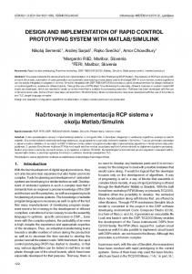
Figure 1: Speedup relative to sequential implementation for 1.2 ∗ 108 iterations. the exception of the four thread runs for the longer run of 1.2 ∗ 109 iterations, where the remote execution on a worker node used 10% more time. In some cases, we see the peculiar behavior of the remote case completing in less time than the local case. We next consider distributing the computation of the Pi estimation over the entire cluster. Specifically, we consider from 1 to 7 worker nodes, and from 1 to 4 threads per worker node. For each of the 28 combinations of number of workers and number of threads per worker, we execute 10 runs, and average the time to estimate Pi over those 10 runs. We repeat for two length runs in number of Monte Carlo samples: 1.2 ∗ 108 and 1.2 ∗ 109 . The results are shown in Figure 1 for the shorter runs, and Figure 2 for the longer runs. These figures show speedup relative to the sequential implementation. The x axis in both graphs is total number of threads. First consider the shorter run length (results of Figure 1). Speedup from parallelizing the computation is approximately linear, regardless of number of threads per worker node, and regardless of number of worker nodes. Vincent A. Cicirello, arXiv:1708.05264v1 [cs.DC], August 2017.

9

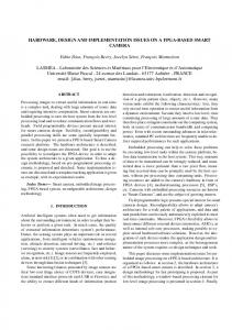
Figure 2: Speedup relative to sequential implementation for 1.2 ∗ 109 iterations.

Next, consider the longer run length (results of Figure 2). For one or two threads per worker node (blue and orange in the graph, respectively), speedup is linear. For three threads per worker (gray in the graph), speedup is very nearly linear, with slightly sublinear speedup at five or more worker nodes (15, 18, or 21 total threads). However, at four threads per worker, speedup is sublinear, with only marginal time improvement from the addition of the fourth thread per worker. Given the Raspberry Pi 3 is quad-core, four threads is hitting the concurrency limit of the processor. The longer run of the experiment shown in this graph is thus more likely to result in contention for the processor from operating system level processes, etc. It is also possible that the longer run with all four processor cores running continuously may be pushing the Raspberry Pi to the temperature (80 degrees Celsius) at which the Pi throttles the CPU clock speed down. I did not record system temperature during the experiment, so I do not know if this is the case. However, I don’t believe this is likely as I would expect the timing results to be further off than they are if the clock speed was cut in half for part of the run. Unlike the case of matrix multiplication, we are able to achieve linear speedup from parallelizing Monte Carlo estimation. The inherent difference between these two tasks that leads to this is that in the case of matrix multiplication, the time required to distribute the matrix strongly dominates the time required for the actual computation, while in the case of Monte Carlo simulation, very little data is transmitted. 10


4

Conclusion

In this report, we describe the implementation of an inexpensive, simple 32 core Raspberry Pi cluster. We explore its performance on a couple easily parallelized computational tasks, one that requires substantial data distribution relative to computational workload, and one that does not. Our results show that a cluster of Raspberry Pi single board computers is significantly limited by its 100 Mbps networking, and is thus not suited to tasks that require distributing a significant amount of data relative to computation time. However, we can achieve linear speedup for tasks that either require very little data transfer among cluster nodes, or that have relatively long run lengths relative to data transfer times. We also observed that speedup from parallelization drops off significantly at four threads per worker node, and recommend limiting concurrency to three threads per worker to minimize resource contention with OS processes.

A

DIY Raspberry Pi Rack from Napkin Holders

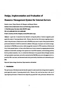
We needed an inexpensive rack-like structure for organizing eight Raspberry Pis in standard cases. For approximately $15, we hacked one together from a couple steel napkin holders, and a bag of zip ties, by doing the following: 1. Use cable/zip ties to hold up the napkin weight on one of the napkin holders so that it is approximately level with the sides of the napkin holder, as in Figure 3(a). 2. The napkin holders that I used have feet that prevent aligning directly atop each other. Rotate the second napkin holder 45 degrees relative to the first. Use cable ties to attach. Make sure you use enough cable ties sufficiently tightened to ensure that the top napkin holder won’t move. Specifically, use two cable ties on each of the three corners that come into contact with the bottom napkin holder. Additionally, use one cable tie to attach the napkin weight of the bottom holder to the bottom of the top holder. See Figure 3(b). 3. Trim the cable ties, as in Figure 3(c). 4. Use cable ties to prop up the napkin weight of the top napkin holder. I connected three cable ties in sequence to span the width of the napkin holder both below and above the napkin weight. I repeated this a couple inches away creating a shelf, which I’m using to hold a network switch. See Figure 3(d). 5. The master node needed more access than the lattice sides of the napkin holder provided. The steel was thin enough to cut off parts of the lattice in the relevant area with a pair of wire cutters, using electrical tape to cover sharp edges that were left behind. This is not pictured in the figure. 6. Each napkin holder is large enough for four raspberry pis in standard cases, each rotated such that ports are accessible via two sides at the corners. You can sit a switch on top of the shelf you created in step 4. I currently have the phone chargers simply sitting next to the rack. Route your power and network cables through the lattice sides of the napkin holders. I used 3 foot long cables, which is partially to blame for the messy wiring in the photo. One foot length cables would be better (and neater). See Figure 3(e). Vincent A. Cicirello, arXiv:1708.05264v1 [cs.DC], August 2017.

11

(a)

(b)

(c)

(d)

(e) Figure 3: DIY Raspberry Pi Rack from Napkin Holders 12


References Adams, J. C., Caswell, J., Matthews, S. J., Peck, C., Shoop, E., and Toth, D. (2015). Budget beowulfs: A showcase of inexpensive clusters for teaching pdc. In Proceedings of the 46th ACM Technical Symposium on Computer Science Education, pages 344–345. ACM. Adams, J. C., Caswell, J., Matthews, S. J., Peck, C., Shoop, E., Toth, D., and Wolfer, J. (2016). The micro-cluster showcase: 7 inexpensive beowulf clusters for teaching pdc. In Proceedings of the 47th ACM Technical Symposium on Computing Science Education, pages 82–83. ACM. Ballard, G., Demmel, J., Holtz, O., Lipshitz, B., and Schwartz, O. (2012). Communication-optimal parallel algorithm for strassen’s matrix multiplication. In Proceedings of the Twenty-fourth Annual ACM Symposium on Parallelism in Algorithms and Architectures, pages 193–204. ACM. Chatterjee, S., Lebeck, A. R., Patnala, P. K., and Thottethodi, M. (1999). Recursive array layouts and fast parallel matrix multiplication. In Proceedings of the Eleventh Annual ACM Symposium on Parallel Algorithms and Architectures, pages 222–231. ACM. Cicirello, V. A. (2017a). Performance tests for small clusters. GitHub. Source code repository: https://github.com/cicirello/ClusterPerformanceTests. Cicirello, V. A. (2017b). Variable annealing length and parallelism in simulated annealing. In Proceedings of the Tenth International Symposium on Combinatorial Search (SoCS 2017), pages 2–10. AAAI Press. Cormen, T., Leiserson, C., Rivest, R., and Stein, C. (2009). Introduction to Algorithms. MIT Press. Hall, L., editor (1892). Beowulf. D.C. Heath and Co. English translation. Karstadt, E. and Schwartz, O. (2017). Matrix multiplication, a little faster. In Proceedings of the 29th ACM Symposium on Parallelism in Algorithms and Architectures, pages 101–110. ACM. Matthews, S. J. (2016). Teaching with parallella: A first look in an undergraduate parallel computing course. Journal of Computing Sciences in Colleges, 31(3):18–27. Neal, D. (1993). Determining sample sizes for monte carlo integration. The College Mathematics Journal, 24(3):254–259. Raspberry Pi Foundation (2017). Raspberry pi: Teach, learn, and make with raspberry pi. Website. https://www.raspberrypi.org/. Sterling, T. L., Savarese, D., Becker, D. J., Dorband, J. E., Ranawake, U. A., and Packer, C. V. (1995). BEOWULF: A parallel workstation for scientific computation. In Proceedings of the 1995 International Conference on Parallel Processing, pages 11–14. Strassen, V. (1969). Gaussian elimination is not optimal. Numer. Math., 13(4):354–356.


13