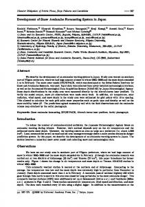
Intl. J. River Basin Management Vol. 1, No. 1 (2003), pp. 49–59 © 2003 IAHR & INBO
Development of a European flood forecasting system AD P.J. DE ROO, BEN GOUWELEEUW and JUTTA THIELEN, Institute of Environment and Sustainability, European Union Joint Research Centre, T.P. 263, 21020 Ispra (VA), Italy JENS BARTHOLMES, PAOLINA BONGIOANNINI-CERLINI and EZIO TODINI, Dipartimento di Scienze della Terra e Geologico-Ambientali, University of Bologna, Piazza di Porta San Donato, 1; via Zamboni, 67 40127 Bologna, Italy PAUL D. BATES∗ , MATT HORRITT and NEIL HUNTER, School of Geographical Sciences, University of Bristol, University Road, Bristol, BS8 1SS, UK. ∗ Contact Author. Tel: +44-117-928-9108; Fax: +44-117-928-7878; E-mail:
[email protected] KEITH BEVEN and FLORIAN PAPPENBERGER, School of Environmental Sciences, University of Lancaster, Lancaster, LA1 4YQ, UK ERDMANN HEISE and GDALY RIVIN, Deutscher Wetterdienst (DWD), Frankfurter Strasse 135, 63067 Offenbach, Germany MICHAEL HILS, Global Runoff Data Centre, Federal Institute of Hydrology, Kaiserin-Augusta-Anlagen 15-17, 56068 Koblenz, Germany ANTHONY HOLLINGSWORTH, European Centre for Medium Range Weather Forecasting (ECMWF), Shinfield Park, Reading RG2 9AX, UK BO HOLST, Swedish Meteorological and Hydrological Institute (SMHI), Folksborgsvagen 1, 60176 Norrkoping, Sweden JAAP KWADIJK, PAOLO REGGIANI and MARC VAN DIJK, WL | Delft Hydraulics, Rotterdamsweg 185, 2629 HD, Delft, The Netherlands KAI SATTLER, Danish Meteorological Institute, Lyngbyvei 100, 2100 Copenhagen, Denmark ERIC SPROKKEREEF, Institute for Inland Water Management and Waste Water Treatment (RIZA), Gildmeesterplein 1, 6826 LL, Arnhem, The Netherlands ABSTRACT Recent advances in meteorological forecast skill now enable significantly improved estimates of precipitation quantity, timing and spatial distribution to be made up to 10 days ahead for model scales of 40 km in forecast mode. Here we outline a prototype methodology to downscale these precipitation estimates using regional Numerical Weather Prediction models to spatial scales appropriate to hydrological forecasting and then use these to drive high-resolution scale (1 or 5 km grid scale) water balance and rainfall-runoff models. The aim is to develop a European Flood Forecasting System (EFFS) and determine what flood forecast skill can be achieved for given basins, meteorological events and prediction products. The output from the system is a probabilistic assessment of n-day ahead discharge exceedence risk (where n < 10) for the whole of Europe at 5 km resolution which may then be updated as the forecast lead time reduces. At each stage the discharge estimates can be used to drive detailed (25–100 m resolution) hydraulic models to estimate the flood inundation which may potentially occur. Initial results are presented from a prototype version of the system used to perform a hindcast of the January 1995 flooding events in NW-Europe (Rhine, Meuse).
Keywords: Flood forecasting; catchment modelling; numerical weather prediction; inundation modelling; uncertainty. 1 Introduction
interest in flood forecasting systems. Some of these periods, such as autumn and winter of 2000/2001 over England and Wales, have been the wettest on record (Marsh, 2001). This has led to speculation that such extremes are attributable in some measure to anthropogenic global warming and represent the beginning of a
Recent large floods, such as those that occurred in the Meuse and Rhine basins in 1995, over large areas of the UK in 1998 and 2000 and in the Elbe basin in summer 2002, have led to heightened
Received and accepted on Jan 17, 2003. Open for discussion until May 31, 2003.
49
50
Ad P.J. De Roo et al.
period of higher flood frequency. Whilst current trends in extreme event statistics will be difficult to discern conclusively until some time in the future, Milly et al. (2002) have shown that for basins greater than 200 000 km2 there was a substantial increase in the frequency of great floods over the 20th Century. There is also increasing evidence (Milly et al., 2002; Palmer and Raisanen, 2002) that anthropogenic forcing of climate change may lead to an increased probability of extreme precipitation, and hence flooding. For example, Palmer and Raisanen (2002) have calculated likely probabilities of extreme precipitation using multimodel ensembles of Global Circulation Model output under baseline and typical enhanced CO2 scenarios. These suggest that the probability of total boreal winter precipitation exceeding two standard deviations above normal will increase by a factor of five over parts of the Northern Europe over the next 100 years. Standard practice in flood forecasting makes use of numerical catchment hydrology models that use measured meteorological variables (precipitation, and sometimes temperature) as boundary condition forcing (e.g. Jasper et al., 2002). The forecast catchment runoff may then itself form a boundary condition for a basin-scale or local scale numerical hydraulic routing model that can then be used to forecast flood stage and discharge at specific locations, and even distributed fields of water depths and velocity where there is access to a suitably resolved Digital Elevation Model (e.g. Baird et al., 1992). For large basins, where flood wave travel times are measured in the order of days, such a system is capable of making adequate forecasts of future water levels in good time for management actions to be undertaken. For example, for the Rhine catchment covering large areas of Switzerland, Germany and The Netherlands, the basin extent means that a recently developed flood forecasting system (Sprokkereef, 2001) based on the above principles is capable of predicting the water level at the Germany/Netherlands border with a lead time of ∼ 4 days. In Europe at least, such a lead time is, however, the exception rather than the rule. Hence, in many situations the desired forecast lead time is longer than the time that a rainfall event takes to pass through the basin. It is therefore necessary to find alternative forcing functions for catchment hydrology models other than observed rainfall as this may not allow for adequate emergency planning. Moreover, there are many flood management actions, such as emptying reservoirs, lowering water levels in rivers, stockpiling emergency supplies and placing key personal on alert, where forecast lead times of greater than the 3–5 days achievable in the largest European basins would be extremely useful, even if these forecasts were probabilistic in nature rather than deterministic. Numerical weather prediction (NWP) models provide a potential solution to this problem. These schemes solve a series of non-linear partial differential equations derived from physical laws for a three dimensional atmosphere with appropriate parameterizations to describe sub-grid physical processes. To begin the calculation, the initial state of the atmosphere at the start of the model run is determined through assimilation of current meteorologic observations. The domain covered may either be global or a particular section of the atmosphere (in which case boundary conditions are required) and is discretized as a grid of
model cells. In the latter case it is possible to use more finely resolved time and space steps, but the model needs to be nested within a global scale model which is used to provide the meteorologic forcing at the boundary. Such systems are capable of predicting values of many atmospheric state variables (including pressure, temperature, humidity, wind speed and direction) for each model grid cell at each time step. Over the last decade the forecast skill of NWP systems has increased significantly (Simmons and Hollingsworth, 2002), both for deterministic forecasts, and increasingly for ensemble forecasts. In ensemble mode up to 50 model realisations are computed, each with slightly different initial conditions to account for uncertainties over the initial data assimilation as modified by the non-linear nature of the atmospheric system. The model results then give an indication of the forecast spread for particular quantities at particular lead times. For example, Buizza et al. (1999) have shown that the European Centre for Medium Range Weather Forecasting (ECMWF) Ensemble Prediction System can give skilful prediction of low precipitation amounts (i.e. lower than 2 mm (12 h)−1 ) up to forecast day 6, and of high precipitation amounts (i.e. between 2 and 10 mm (12 h)−1 ) up to day 4. Whilst these figures are lower than typical rainfall rates during major flooding episodes (up to 50 mm (12 h)−1 ), Buizza and Hollingsworth (2002) have shown that the Ensemble Prediction System can give early indications of possible severe storm occurrence. Moreover, they showed that the probabilistic ensemble forecasts were especially useful when the deterministic forecasts issued on successive days were highly inconsistent. Chessa and Lalaurette (2001) have also shown that in terms of replicating large scale atmospheric flow patterns, the ensemble forecasts have positive skill scores with respect to the deterministic reference forecast for up to 10 days ahead. Forecast skill with NWP systems has now advanced to a state where significantly improved estimates of precipitation quantity, timing and spatial distribution can be made up to 10 days ahead for model scales of 40 km in deterministic mode and 80 km in ensemble mode. It is now appropriate to ask whether this improvement is yet capable of yielding meaningful flood forecasts and determine what flood forecast skill can be achieved for given basins, meteorological events and prediction products. This is the question we begin to address in this paper where we describe the development of a European-scale flood forecasting system. An overview of the modelling system is given in Section 2, along with a description of the data available to run the model at a European scale at up to 1 km resolution in Section 3. Finally, Section 4 presents initial results from a prototype version of the system used to perform a hindcast of the January 1995 flooding events in NW-Europe (Rhine, Meuse).
2 The European Flood Forecasting System (EFFS) The European Flood Forecasting System prototype consists of the following components: 1. global Numerical Weather Prediction models,
Development of a European flood forecasting system
2. optional downscaling of global precipitation from (1) using a regional Numerical Weather Prediction model, 3. a catchment hydrology model comprising a soil water balance model with daily time step and a flood simulation model with hourly time step, 4. a high-resolution flood inundation model. These are integrated within a generic modelling framework that allows different models to be used interchangeably for each component. The modelling framework is linked to a central database and is mounted on an open, platform-independent architecture, that allows encapsulation of various pre-existing simulation codes via appropriate “model wrappers”. The wrappers convert input data such as time series and parameters from the main database to a format readable by the particular model, and store model results back in the main database. Hence, although the hydrology and hydraulic components of the system (3–4 above) have been based around the LISFLOOD suite of raster-based hydrology and hydraulic codes (De Roo et al., 2000, 2001; Bates and De Roo, 2000; Horritt and Bates, 2001) other models can alternatively be used. Thus within the project the well known HBV (Bergström, 1976; Harlin, 1992; Bergström et al., 2002) and TOPKAPI (Ciarapica and Todini, 2002) catchment hydrology codes have also been implemented and tested for particular basins. This was considered desirable to allow end-users to implement the system with their own models which may be better suited to local conditions, and also to allow comparison of results from the EFFS with existing operational software. For regions where local models do not exist, the LISFLOOD suite is available as a default option.
2.1 The ECMWF global NWP model Large scale weather forecasts for the EFFS system are derived using the European Centre for Medium Range Weather Forecasting Ensemble Prediction System (Molteni et al., 1996). This is a primitive equation atmospheric General Circulation Model model which solves the equations of continuity for mass and momentum, a gas law which gives the relation between pressure, density and temperature, a hydrostatic equation for the relationship between the air density and change of pressure with height, a thermodynamic equation and a conservation equation for moisture. Sub-grid scale processes, such as topographic effects, exchanges of momentum, heat and moisture with the land surface, the hydrological cycle, cloud formation and cloud-radiation interaction are all represented through appropriate parameterizations. The model initial state is determined through two fourdimensional variational data assimilation cycles. The analysis is performed by comparing the observations directly with a very short forecast, using exactly the same model as the operational medium-range forecast. The differences between the observed values and the equivalent values predicted by the short-range forecast are used to make a correction to the first-guess field in order to produce the atmospheric analysis (Courtier et al., 1994).
51
The model equations are solved every 15 min, with the time step chosen in order to avoid numerical instabilities and ensure enough accuracy. The vertical resolution is highest in the planetary boundary layer and lowest in the stratosphere and lower mesosphere. The atmosphere is divided into 60 layers up to 0.1 hPa (about 64 km above the surface). These so-called σ -levels follow the earth’s surface in the lower and mid-troposphere and are used as vertical co-ordinates, but are surfaces of constant pressure in the upper stratosphere and mesosphere. The horizontal resolution is based on a spherical harmonic expansion, truncated at total wave number 511 for the deterministic forecast (the TL511L60 model) which equates to an approximate horizontal resolution of 40 km. In ensemble mode the horizontal and vertical resolutions are reduced to 255 spectral components and 40 vertical levels up to 10 hPa (the TL255L40 model) to allow a tractable computational problem. This gives an approximate horizontal resolution of 80 km. For the ensemble forecasts a control and 50 perturbations are computed independently for both the Northern and the Southern Hemisphere with the different initial states assumed a priori to be equally likely. The EPS perturbation technique is based on singular vector analysis and tries to identify the dynamically most unstable regions of the atmosphere by calculating where small initial uncertainties would affect a 48 h forecast most rapidly (Buizza and Palmer, 1995). In either mode, the resulting system produces a forecast of weather variables (e.g. 2 m temperature, 10 m wind and precipitation) usually archived for each grid cell every 6 hours for up to 10 days ahead. 2.2 The DMI and DWD global and regional NWP models To increase forecast spatial and temporal resolution, regional NWP models with lead times of up to 3 days can be used to downscale the output from global NWP models. Such models represent a limited area of the Earth’s surface with boundary conditions at the edges of the domain being provided by a global scale model. For EFFS, two such regional NWP models are available: the DMI version of the High Resolution Local Area Model (HIRLAM) developed jointly by the Meteorological Institutes in Norway, Finland, Sweden, Denmark, Iceland, Ireland, Spain and the Netherlands as well in collaboration with Météo-France (Källen, 1996; Sass et al., 2000, Undén et al., 2002) and the “Lokal-Modell” (LM) (Damrath et al., 2000; Steppeler et al., 2003) developed by the German Weather Service (Deutscher Wetterdienst or DWD). The spatial extents of the DMI and DWD models, as well as the extent of the data retrieved from the ECMWF-EPS archive are shown in Figure 1. The DMI-HIRLAM model is a hydrostatic grid-point model with high spatial resolution. It is based on the same set of atmospheric equations as the global ECMWF model and includes several parameterization schemes for the treatment of the subgrid physical processes. The model is used at DMI for daily NWP (Sass et al., 2002). In the context of EFFS the model is established as a doubly 1-way nested set of models, of which the innermost model uses a horizontal grid of 0.1◦ (∼11 km horizontal grid spacing) covering the whole of Europe. The boundary conditions for the outermost model are retrieved from the ECMWF archive.
52
Ad P.J. De Roo et al.
Figure 1 Spatial extent of the meteorological models used in the EFFS system. The DWD-LM model extent is shown in purple, the DMI-HIRLAM model extent in pale green and bounding box for the ECMWF-EPS archive retrieval in bright green.
Forecasts are produced with an hourly data output for up to 72 h ahead (Sattler, 2002). Unlike the other models, the DWD-LM uses a non-hydrostatic representation of the atmosphere for a grid covering western Europe only at a horizontal resolution of 0.0625◦ or ∼7 km and with 35 vertical layers. For the non-hydrostatic component two additional prognostic equations are solved for the vertical wind speed and the pressure deviation. The vertical turbulent diffusion calculation is based on a level 2.5 scheme solving an additional prognostic equation for the turbulent kinetic energy (TKE). It includes a laminar sublayer at the earth’s surface. Boundary conditions are provided by the DWD’s own global scale hydrostatic grid-point model (DWD-GME) with ∼55 km horizontal resolution and 31 vertical layers (Majewski et al., 2002). Forecasts with the DWD-GME are produced for up to 156 h ahead with a 6 h output. Forecasts with the DWD-LM model are then produced with an hourly output for up to 48 h ahead. The forecasts from the limited-area models comprise a similar set of variables to the forecasts from the global models, but adopting a shorter forecast range. The higher spatial and temporal resolution of these models allows, however, for the inclusion of more detailed data (e.g. orography and surface type) and for an enhanced spectrum of resolved physical scales towards smaller scales. Hence, they are likely to provide more realistic weather predictions than the coarse scale global models. 2.3 Catchment hydrology models The EFFS modelling framework imports data from each different meteorological grid and converts it to a common format
for use by large-scale hydrological models. The default model for this component is the LISFLOOD suite of raster-based catchment hydrology models being developed by the European Commission Joint Research Centre (De Roo et al., 2000, 2001). LISFLOOD simulates runoff and flooding in large river basins as a consequence of extreme rainfall. The code is a distributed rainfall-runoff model which takes into account the influence of topography, precipitation amounts and intensities, antecedent soil moisture content, land use type and soil type. LISFLOOD simulates flood events – typically up to a 1.5 month duration and including a pre-flood period of typically 1 year duration simulated with a daily time step – in catchments using various pixel sizes (1 km or smaller) and with various time steps (1 h or shorter). A flowchart of the model describing the main processes simulated and links to the floodplain hydraulic model is shown in Figure 2. Interception of rainfall by vegetation is simulated using the method of Von Hoyningen-Huene (1981) for all land use except forests, for which the approach of Shuttleworth and Calder (1979) is used. The equations are based on the Leaf Area Index of the vegetation. Seasonal changes of LAI are taken into account. Evapotranspiration is simulated using the Penman-Monteith method, as applied in the WOFOST model (Supit et al., 1994; Van Der Goot, 1997). For forests, the Priestley-Taylor equation is used, as modified by Shuttleworth and Calder (1979). In forecast mode, large scale and convective precipitation, air temperature at 2 m reference height and latent heat flux are provided gridded by the meteorological models. The data are corrected making use of the higher resolution topography as opposed to the comparatively coarse meteorological grids. The Leaf Area Index of each simulated pixel is used to calculate actual evapotranspiration
Development of a European flood forecasting system
53
Figure 2 Flowchart of the three LISFLOOD model components, their inputs and their products.
from potential evapotranspiration. Snowmelt is simulated using a degree-day method (Baumgarter et al., 1994), when the average daily temperature is above 0◦ C. Infiltration is simulated using the Smith-Parlange equation (Smith and Parlange, 1978). The capillary drive value is based on topsoil texture. Saturated hydraulic conductivity values are based on topsoil texture and land use. A correction factor is applied to account for land use influences on infiltration. For example, in urban areas and on open water surfaces no infiltration takes place. Soil freezing is simulated using a degree-day method (Molnau and Bissel, 1983). If the soil is frozen to a certain degree, infiltration is reduced to zero. Vertical transport of water in the two soil layers is simulated using a onedimensional form of the Richard’s equation. Soil water retention and conductivity curves are described by van Genuchten’s (1980) relationships. Pedotransfer-functions from the HYPRES project (Wösten et al., 1998) are used to calculate the water retention and conductivity curves from soil texture. Both soil texture and soil depth are derived from the European Soils Database (Finke et al., 1998) or local soil maps. Percolation to the groundwater store is calculated using the Darcy equation. Hydrological forecasts are produced by first running the model for a long antecedent period (1–5 years) of observed precipitation with a daily time step to calculate catchment water balances and realistic spatial distributions of soil moisture at the start of the forecast period. The outputs from the long-term water balance model (LISFLOOD-WB) then form the initial conditions for the flood forecasting model (LISFLOOD-FF). This uses identical model physics and grid resolution as LISFLOOD-WB, but at an hourly time step and with precipitation boundary conditions derived from the NWP forecasts. Numerous outputs are available from the system and include soil moisture contents in each grid cell, predicted flow and stage hydrographs for any point on the drainage network, flood source areas and estimates of groundwater recharge.
An important part of the EFFS-project was also to evaluate the performance and reliability of flood forecasts for 10 days compared to the lead-times typically used in operational forecasting. Therefore calibration, verification and comparison of several local and specialised models are essential aspects of the project work. To achieve this several catchments have been selected representing various hydrological behaviours as well as impact from the different weather systems in different parts of Europe. Among rivers to be tested are the Helgå and Viskan in Sweden, the Rhine and Meuse in Germany and the Netherlands, the Severn in the UK and the Po in Italy. In the case of Sweden, the HBV model was tested for two catchments in the southern part of the country having a mixed run-off regime, where a combination of snowmelt and rainfall produces high and sometimes extreme floods during the period October to February. A comparison of the operationally used and rigorously calibrated HBV model with the large scale GIS-based LISFLOOD approach will provide valuable experience for further development of models and methods in Sweden. A similar comparison is taking place for the Po catchment between LISFLOOD and the TOKAPI model. 2.4 Floodplain hydraulic model In order to translate a point hydrograph forecast, as produced by LISFLOOD-FF, into products for use by environmental agencies and civil protection authorities some hydraulic model is necessary. For the EFFS project a simple two-dimensional hydraulic model has been developed within the LISFLOOD framework, for application to river-floodplain reaches up to 100 km in length and at spatial scales of 10–100 m (Bates and De Roo, 2000; Horritt and Bates, 2001). The model, LISFLOOD-FP, solves a one-dimensional kinematic wave equation for in-channel flow using an explicit finite difference scheme. Once water depths in the channel exceed bankful depth, water is transferred to
54
Ad P.J. De Roo et al.
floodplain sections adjacent to the channel. As with other models in the LISFLOOD suite, the floodplain is discretized as a raster grid with the floodplain elevation at each point initialised from a high-resolution topographic survey derived using such techniques as airborne laser altimetry (Richie, 1996; Gomes-Pereira and Wicherson, 1999). Each model grid square on the floodplain is then treated as a storage cell (after Cunge et al., 1976), with fluxes between each cell calculated explicitly using simple uniform flow formulae driven by water surface gradient and topography. The model takes as its input a flow hydrograph at the head of the reach of interest derived from either observed gauging station data or the LISFLOOD-FF model. As a kinematic in-channel equation is used there is no need for a downstream boundary condition. The output from the model consists of the water depth in each grid cell at each time step. This representation of floodplain flow physics is thus able to predict the dynamic wetting and drying of the floodplain in response to extreme discharge events and provide forecasts of time-varying water depths and inundation extent that can be used by catchment managers and civil protection authorities.
3 Model inputs and uncertainty For meteorological models an internationally agreed system of data acquisition and sharing is co-ordinated through the World Meteorological Organisation (WMO). This is not the case for hydrological models and for the EFFS project an appropriate data collection and transfer system for river flows has been developed by the Global Runoff Data Centre. This consists of a regularly updated database containing time series of historic daily river discharge for many stations. The aim is for the database to contain all the information for the calibration and validation of the hydrological forecast models. The historical data set available for EFFS consists at present of 257 time series from 16 European countries. In addition, 6 countries also provide near real-time discharge data from a total of 168 stations and a internet-based system for their distribution within EFFS has been developed by the GRDC. Other inputs for the hydrological models are derived from published data sources held either by National agencies or by European-level institutions. These are corrected to an identical projection and interpolated to the model grid. For example, 1 km resolution DEM, soil, land use (CORINE) and drainage network databases with full European coverage now exist. Figures 3 and 4 show the level of detail now available at this scale in all hydrological model input areas. It must also be noted that dealing with uncertainty in such a complex system of linked numerical codes and databases is a major research area in its own right. Not only will there be uncertainty over the input and validation data, but also over the model parameters and conceptual basis (see Beven, 2002 for a discussion). Numerous sources of error will cascade through the modelling chain, possibly in a non-linear interacting fashion. Developing computationally tractable methods of estimating the uncertainty resulting from these various sources is therefore also a key aspect of the project.
DEM
Land use
Soil texture
Soil depth
Figure 3 Hydrology model inputs from databases held by National and European-level agencies.
4 Application to the 1995 River Meuse floods Initially, the system has been used to model a period in January 1995 (Figure 5) when major flooding occurred along a number of European rivers. For the Meuse, this comprised an event with an estimated recurrence interval of 1 in 63 years and with maximum discharge in downstream reaches approaching 3000 m3 s−1 . To simulate this event the water balance model was first run and calibrated for the whole of Europe at 5 km resolution for the period 1992–5 using observed precipitation data. Simulations were then attempted using LISFLOOD-FF for the Meuse basin upstream of the Borgharen gauging station in The Netherlands at 1 km resolution using both measured and ECMWF deterministic and Ensemble Prediction System 10 day ahead, forecast data as model boundary conditions. Hindcast simulations using LISFLOOD-FF commenced at 00:00 h UTC on 19th January 1995 and were run for the observed meteorologic data, the deterministic forecast, the ensemble control and each ensemble member, giving 53 simulations in all. This set of simulations was then repeated on each subsequent day and the output from the model compared to the observed flow at the Borgharen gauge. The first major flood peak occurred on the 27th January, and from this time flow was continuously above 2500 m3 s−1 until the 2nd February. During this period a further flood peak passed by the gauge on the 31st January. Figure 6 shows the hydrological forecasts made starting on 19th January. These results show the hydrological model to be capable of simulating the observed flow at Borgharen when forced with the observed meteorological data. The simulation driven with the deterministic forecast (TL511L60) captures the minor flood peak on the 24th at 5 days ahead, but thereafter fails to capture the main body of the flood. The majority of the ensemble members and the ensemble control miss both the first minor peak on the 24th and the main flood hydrograph commencing on the 27th, however the spread of ensemble members does indicate at least the possibility of an extreme event towards the end of the 10 day forecast period.
Development of a European flood forecasting system
55
Figure 4 Part of the Joint Research Centre Europe-wide river network database to show detail achievable in public domain data.
Precipitation
Evapotranspiration
Groundwater recharge
Overland flow
Figure 5 Simulation of the 1995 River Meuse flood event using the LISFLOOD-WB (upper panel) and LISFLOOD-FF (lower panel) models at 5 km and 1 km resolution respectively.
56
Ad P.J. De Roo et al.
Figure 6 10-day discharge forecasts from the LISFLOOD-FF model for 0000 UTC on 19th January 1995 (hour 0) for the Borgharen gauging station on the River Meuse, The Netherlands. The observed discharge is shown as a thick blue line, the simulation driven by observed meteorologic data is shown as a thin blue line, the simulation driven by the ECMWF TL511L60 deterministic forecast is shown in red, the simulation driven by the ECMWF TL255L40 ensemble control forecast is shown in green and the simulations driven by the 50 ECMWF TL255L40 ensemble forecast members are shown in black.
Figure 7 10-day discharge forecasts from the LISFLOOD-FF model for 0000 UTC on 21st January 1995 (hour 48) for the Borgharen gauging station on the River Meuse, The Netherlands. The observed discharge is shown as a thick blue line, the simulation driven by observed meteorologic data is shown as a thin blue line, the simulation driven by the ECMWF TL511L60 deterministic forecast is shown in red, the simulation driven by the ECMWF TL255L40 ensemble control forecast is shown in green and the simulations driven by the 50 ECMWF TL255L40 ensemble forecast members are shown in black.
Figure 7 shows the updated forecast made on the 21st January with a similar prediction skill achieved using the observed meteorologic data. In this instance, the deterministic forecast, ensemble control and ensemble members all capture the minor peak on the 24th, and some correctly predict the main body of the flood from
forecast day 5 onwards. Most simulations, however, still tend to underestimate the observed flow during the main flood pulse, although the observed discharge is exceeded by 1 or 2 ensemble members. Figure 8 shows a possible way to interpret the data from the EFFS system by calculating cumulative distribution
Development of a European flood forecasting system
57
Figure 8 Interpretation of 10-day discharge forecasts from the LISFLOOD-FF model for 0000 UTC on 21st January 1995 (hour 48) for the Borgharen gauging station on the River Meuse, The Netherlands driven by the ECMWF Ensemble Prediction System. The observed discharge is shown as a thick blue line. 25% (Q1), 50% (Q2), 75% (Q3) and 100% (Q4) quartiles for the 51 EPS ensemble members are shown, the 50% corresponding to the median value. The simulations show that the system provides a good forecast of discharge up to 5 days ahead and a probabilistic assessment of extreme flooding for forecast lead times in the range 5–10 days.
valley below the Borgharen gauging station. For this reach a high-resolution topographic survey has been conducted by RWS Maastricht and can therefore be used to define the floodplain geomtery. The simulation is driven using the observed flow from the Borgharen gauging station and is compared to an observed inundation extent derived from oblique aerial photography taken on 27th January when the flow was 2645 m3 s−1 . The model was run with at 50 m resolution with a 5 s time step and correctly classifies inundation extent in 85% of model grid cells.
5 Conclusions Figure 9 Predicted water depths and inundation extent simulated using the LISFLOOD-FP applied at 50 m resolution to the 35 km river-floodplain reach below the Borgharen gauging station, River Meuse, The Netherlands over 20 days of the January 1995 event. Observed flow at the gauging station from the 19th January is used as a model boundary condition and predicted inundation is compared to that observed by aerial photography taken on 27th January. The model correctly classifies as wet or dry 85% of pixels in the above image.
(represented here as quartiles) of the ensemble forecasts at each archive time. This shows that the EPS average provides a good simulation of flow for this event up to forecast day 5, and a probabilistic assessment of extreme flooding for forecast lead times in the range 5–10 days. Lastly, Figure 9 shows a prediction of water depth and flood extent from the LISFLOOD-FP model for 35 km of the Meuse
In this paper we have described the development of a Europeanscale flood forecasting system (EFFS) and an initial hindcast of the River Meuse flooding event of January 1995. Even using the coarse resolution meteorologic forecasts from the ECMWF deterministic and Ensemble Prediction System model runs to drive the LISFLOOD simulations in the Meuse basin achieved a number of encouraging results to be achieved. This preliminary work requires confirmation for other basins and flood events, however the general principles and potential utility of the system are apparent. It is also likely that for shorter forecast lead times using meteorologic forecasts downscaled using a regional NWP model that even better forecast skill can be achieved. It is also clear that with an adequate prediction of at-a-point discharge we should be able to achieve reasonable predictions of hydraulic variables such as water depth and inundation extent over relatively long river reaches. Much further work remains to document and analyse the performance of the system, and in particular, a major research
58
Ad P.J. De Roo et al.
challenge should be the development of computationally tractable techniques to analyse how uncertainties cascade through a chain of linked non-linear models. However, there does appear to be considerable scope for the development of useful medium-range flood prediction products.
Acknowledgements This project was funded by the European Union Framework 5 grant “Development of a European Flood Forecasting System”. Our thanks go to the RWS Maastricht for allowing access to the air photo inundation extent data, DEM, surveyed cross sections and flow discharge data from the Borghren gauging station.
References 1. Baird, L., Gee, D.M. and Anderson, M.G. (1992). “Ungauged Catchment Modelling 2: Utilization of Hydraulic Models for Validation”, Catena, 19, 33–42. 2. Bates, P.D. and De Roo, A.P.J. (2000). “A Simple Rasterbased Model for Floodplain Inundation”, J. Hydrology, 236, 54–77. 3. Baumgartner, M.F., Martinet, J., Rango, A. and Roberts, R. (1994). Snowmelt Runoff Model (SRM) User’s Manual. Univeristy of Bern. Dept. of Geography. 4. Bergström, S. (1976). Development and Application of a Conceptual Runoff Model for Scandinavian Catchments. Swedish Meteorological and Hydrological Institute, Report RHO, No. 7, Norrköping, Sweden. Ph.D. thesis. 5. Bergstrom, S., Lindstrom, G. and Pettersson, A. (2002). “Multi-variable Parameter Estimation to Increase Confidence in Hydrological Modelling”, Hydrological Processes, 16, 413–421. 6. Beven, K. (2002). “Towards a Coherent Philosophy for Modelling the Environment”, Proceedings of the Royal Society of London Series A – Mathematical, Physical and Engineering Sciences, 458, 2465–2484. 7. Buizza, R, and Palmer, T.N. (1995). “The Singularvector Structure of the Atmospheric General circulation”, J. Atmospheric Science, 52, 1434–1456. 8. Buizza, R. and Hollingsworth, A. (2002). “Storm Prediction Over Europe Using the ECMWF Ensemble Prediction System”, Meteorological Applications, 9(3), 289–305. 9. Buizza, R., Hollingsworth, A., Lalaurette, E. and Ghelli, A. (1999). “Probabilistic Predictions of Precipitation Using the ECMWF Ensemble Prediction System”, Weather and Forecasting, 14(2), 168–189. 10. Chessa, P.A. and Lalaurette, F. (2001). “Verification of the ECMWF Ensemble Prediction System Forecasts: A Study of Large-scale Patterns”, Weather and Forecasting, 16(5), 611–619. 11. Ciarapica, L. and Todini, E. (2002). “TOPKAPI: A Model for the Representation of the Rainfall-runoff Process at Different Scales”, Hydrological Processes, 16, 207–229.
12. Courtier, P., Thépaut, J.-N. and Hollingsworth, A. (1994). “A Strategy for Implementation of 4DVAR Using an Incremental Approach”, Quarterly J. Royal Meteorological Society, 120, 1367–1388. 13. Cunge, J.A., Holly, F.M. Jr. and Verwey, A. (1976). Practical Aspects of Computational River Hydraulics. Pitman, London. 14. Damrath, U., Doms, G., Frühwald, D., Heise, E., Richter, B. and Steppeler, J. (2000). “Operational Quantitative Precipitation Forecasting at the German Weather Service”, J. Hydrology, 239, 260–285. 15. De Roo, A., Odijk, M., Schmuck, G., Koster, E. and Lucieer, A. (2001). “Assessing the Effects of Land Use Changes on Floods in the Meuse and Oder Catchment”, Physics and Chemistry of the Earth, Part B – Hydrology, Ocean and Atmosphere, 26, 593–599. 16. De Roo, A.P.J., Wesseling, C.G. and Van Deursen, W.P.A. (2000). “Physically Based River Basin Modelling within a GIS: The LISFLOOD Model”, Hydrological Processes, 14, 1981–1992. 17. Finke, P., Hartwich, R., Dudal, R., Ibanez, J., Jamagne, M., King, D., Montanarella, I. and Yassoglou, N. (1998). Geo-referenced Soil Database For Europe – Manual ’of Procedures Version 1. European Soil Bureau Scientific Committee, Office for Official Publications of the European Communities, Luxembourg. Report no. EUR 18092 EN, p. 184. 18. Gomes-Pereira, L.M. and Wicherson, R.J. (1999). “Suitability of Laser Data for Deriving Geographical Data: A Case Study in the Context of Management of Fluvial Zones”, Photogrammetry and Remote Sensing, 54, 105–114. 19. Harlin, J. (1992). “Modelling the Hydrological Response of Extreme Floods in Sweden”, Nordic Hydrology, 23, 227–244. 20. Horritt, M.S. and Bates, P.D. (2001). “Predicting Floodplain Inundation: Raster-based Modelling versus the Finite Element Approach”, Hydrological Processes, 15, 825–842. 21. Jasper, K., Gurtz, J. and Herbert, L. (2002). “Advanced Flood Forecasting in Alpine Watersheds by Coupling Meteorological Observations and Forecasts with a Distributed Hydrological Model”, J. Hydrology, 267(1–2), 40–52. 22. Källen, E. (1996). HIRLAM Documentation Manual. Swedish Meteorological and Hydrological Institute, Norrköping, Sweden. 23. Majewski, D., Liermann, D., Prohl, P., Ritter, B., Buchhold, M., Hanisch, Th., Paul, G., Wergen, W. and Baumgardner, J. (2002). “The Operational Global Icosahedral-hexagonal Gridpoint Model GME: Description and High-resolution Tests”, Monthly Weather Review, 130(2), 319–338. 24. Marsh, T.J. (2001). “The 2000/01 Floods in the UK: A Brief Overview”, Weather, 56, 343–345. 25. Milly, P.C.D., Wetherald, R.T., Dunne, K.A. and Delworth, T.L. (2002). “Increasing Risk of Great Floods in a Changing Climate”, Nature, 415, 514–517.
Development of a European flood forecasting system
26. Molnau, M. and Bissel, V.C. (1983). “A Continuous Frozen Ground Index for Flood Forecasting”, Proceedings of the 5lst Annual Meeting of the Western Snow Conference, 109–119. 27. Molteni, F., Buizza, R., Palmer, T.N. and Petroliagis, T. (1996). “The New ECMWF Ensemble Prediction System: Methodology and Validation”, Quarterly J. Royal Meteorological Society, 122, 73–119. 28. Palmer, T.N. and Raisanen, J. (2002). “Quantifying the Risk of Extreme Seasonal Precipitation Events in a Changing Climate”, Nature, 415, 512–514. 29. Ritchie, J.C. (1996). “Remote Sensing Applications to Hydrology: Airborne Laser Altimeters”, Hydrological Sciences J., 41, 625–636. 30. Sass, B.H., Nielsen, N.W., Jörgensen, J.U., Amstrup, B. and Kmit, M. (2000). The Operational DMI-HIRLAM System. Danish Meteorological Institute Technical Report 00-26. Available from www.dmi.dk. 31. Sass, B.H., Nielsen, N.W., Jørgensen, J.U., Amstrup, B., Kmit, M. and Mogensen, K.S. (2002). The Operational DMI-HIRLAM System 2002-version. Danish Meteorological Institute Technical Report, 02-05. Available from www.dmi.dk. 32. Sattler, K. (2002). Precipitation Hindcasts of Historical Flood Events. DMI Sci. Rep., 02-13. Available from the Danish Meteorological Institute (DMI) Copenhagen, Denmark. 33. Shuttleworth, W.S. and Calder, I.R. (1979). “Has the Priestley-Taylor Equation any Relevance to Forest Evaporation?”, J. Applied Meteorology, 18, 639–646. 34. Simmons, A.J. and Hollingsworth, A. (2002). “Some Aspects of the Improvement in Skill of Numerical Weather Prediction”, Quarterly J. Royal Meteorological Society, 128, 647–677. 35. Smith, R.E. and Parlange, J.Y. (1978). “A Parameterefficient Hydrologic Infiltration Model”, Water Resources Research, 14, 533–538. 36. Sprokkereef, E. (2001). Extension of the Flood Forecasting Model FloRIJN. NCR publication 12-2001. ISSN no. 1568234X.
59
37. Steppeler, J., Doms, G., Schättler, U., Bitzer, H.W., Gassmann, A., Damrath, U. and Gregoric, G. (2003). “Meso-gamma Scale Forecasts Using the Nonhydrostatic Model LM”, Meteorology and Atmospheric Physics, in press. 38. Supit, I., Hooijer, A.A. and Van Diepen, C.A. (1994). System Description of the Wofost 6.0 Crop Simulation Model Implemented in CGMS. Volume I: Theory and Algorithms. European Commission, Joint Research Centre, Report no. EUR 15956 EN. 39. Undén, P., Rontu, L., Järvinen, H., Lynch, P., Calvo, J., Cats, G., Cuxart, J., Eerola, K., Fortelius, C., Antonio Garcia-Moya, J., Jones, C., Lenderlink, G., McDonald, A., McGrath, R., Navascues, B., Woetman Nielsen, N., Ødegaard, V., Rodriguez, E., Rummukainen, M., Rõõoom, R., Sattler, K., Sass, B.H., Savijäarvi, H., Wichers Schreur, B., Sigg, R., The, H. and Tijm, A. (2002). HIRLAM-5 Scientific Documentation, Swedish Meteorological and Hydrological Institute, Norrköping, Sweden. 40. Van Der Goot, E. (1997). Technical Description of Interpolation and Processing of Meteorological Data in CGMS. Joint Research Centre, Space Applications Institute, Ispra, Italy, Internal Report. 41. Van Genuchten, M.Th. (1980). “A Closed-form Equation for Predicting the Hydraulic Conductivity of Unsaturated Soils”, Soil Science Society of America J., 44, 892– 898. 42. Von Hoyningen-Huene, J. (1981). Die Lnterzeption Des Niederschlags in landwirtschaftlichen Pflanzenbeständen. Arbeitsbericht Deutscher Verband für Wasserwirtschaft und Kulturbau, DVWK, Braunschweig, Germany, p. 63. 43. Wöten, J.H.M., Lilly, A., Nemes, A. and Le Bas, C. (1998). Using Existing Soil Data to Derive Hydraulic Parameters for Simulation Models in Environmental Studies and in Land Use Planning. Winand Staring Centre, Wageningen, The Netherlands Report no. 156, p. 106.