ECHTZEITOPTIMIERUNG GROSSER SYSTEME
F. L EHN , B. T IBKEN , AND E. P. H OFER
Development of a Simulation Environment for Time Delay Differential Equations
Preprint 98-29
SCHWERPUNKTPROGRAMM DER DEUTSCHEN FORSCHUNGSGEMEINSCHAFT
Development of a Simulation Environment for Time Delay Differential Equations Frank Lehn∗, Bernd Tibken, and Eberhard P. Hofer University of Ulm Department of Measurement, Control and Microtechnology D-89069 Ulm, Germany
Abstract In this paper the development of a simulation environment for time delay differential equations will be presented. After the analysis of the mathematical foundations, the practical implementation using the C++ programming language will be discussed. Simulations of a biomathematical time delay model of the human granulopoiesis are presented and the paper concludes with an error analysis and a discussion of simulation execution times.
1
Introduction
Delay differential equations (DDE) are used to model a variety of phenomena in the physical and natural sciences [1, 2, 3, 4, 5, 6, 7, 8, 9, 10, 11]. Also in the modeling of biological systems time delays occur which can be modeled using DDEs. Because of this large number of applications it is of special interest to develop a simulation tool for DDEs. In previous work of Feldstein and Neves [1] high-order methods for the integration of DDEs with time and state dependent time delays have been derived. In this paper we concentrate on the numerical implementation of these methods using the C++ programming language where the class concept will be presented. The analysis of dicretization errors will show high accuracy while simulation results show excellent efficiency of our implementation. We consider time delay differential equations with state vector x(t) = (x1 (t), ..., xn (t))T and state space representation x˙i (t) = fi (t, x(t), x(α1 (t, x(t))), . . . , x(αr (t, x(t)))) for t ∈ [t0 , te ] , i = 1, ..., n
(1)
with r retarding functions αj (t, x(t)) ≤ t ∀ t ∈ [t0 , te ] , j = 1, ..., r ∗
Corresponding author. Phone ++49 731 50-26323, Fax ++49 731 50-26301, Email
[email protected]
1
(2)
which are allowed to depend on time and state. The initial value problem is given by an initial function x(t) = Φ(t) for t ≤ t0 (3) which describes the history of the solution. In general the solution is non-smooth, which means that discontinuities occur in the higher order derivatives of the solution. Practically this is due to the non-smooth transition at the starting point t0 and the propagation of this non-smoothness which depends upon the retarding functions.
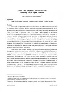
Start x(t)=φ(t), t≤t0 Z1=t0, j=0, i=1
Is j