Distributed Algorithms for Lifetime of Wireless Sensor Networks Based ...

Distributed Algorithms for Lifetime of Wireless Sensor Networks Based on Dependencies Among Cover Sets Sushil K. Prasad and Akshaye Dhawan Computer Science Department Georgia State University Atlanta, GA 30303, U.S.A {sprasad, akshaye}@cs.gsu.edu Abstract. We present a new set of distributed algorithms for scheduling sensors to enhance the total lifetime of a wireless sensor network. These algorithms are based on constructing minimal cover sets each consisting of one or more sensors which can collectively cover the local targets. Some of the covers are heuristically better than others for a sensor trying to decide its own sense-sleep status. This leads to various ways to assign priorities to the covers. The algorithms work by having each sensor transition through these possible prioritized cover sets, settling for the best cover it can negotiate with its neighbors. A local lifetime dependency graph consisting of the cover sets as nodes with any two nodes connected if the corresponding covers intersect captures the interdependencies among the covers. We present several variations of the basic algorithmic framework. The priority function of a cover is derived from its degree or connectedness in the dependency graph - usually lower the better. Lifetime improvement is 10% to 20% over the existing algorithms, while maintaining comparable communication overheads. We also show how previous algorithms can be formulated within our framework.

1 Introduction Wireless sensor networks (WSNs) are emerging as a key enabling technology for applications domains such as military, homeland security, and environment [7]. For example, in typical security surveillance or environmental monitoring scenarios, tiny low-cost radio-enabled sensors can be deployed in large numbers over a difficult or hostile terrain. Then, they configure themselves into a network to collectively sense and route data to gateway nodes. Interested readers are referred to [1] [7] for detailed background, applications and challenges of WSNs. The sensors, by design, have limited battery. Therefore, they must conserve power while communicating, sensing, and computing. One key challenge is to utilize the network effectively to maximize the duration of time while all the targets (or alternatively certain area [9]) can be continuously monitored. This duration is called the lifetime of the network, which is the concern of this paper. Only a subset of sensors usually need to be in “sense” or “on” mode at any given time to cover all the targets (henceforth called “covers” – See Section 2 for a formal definition), while others can go into power conserving “sleep” or “off” mode. Therefore, an ideal sensesleep schedule would choose appropriate covers at various intervals to maximize the lifetime. Thus, at its heart, this is an NP-complete problem [6] [8]. S. Aluru et al. (Eds.): HiPC 2007, LNCS 4873, pp. 381–392, 2007. © Springer-Verlag Berlin Heidelberg 2007

382

S.K. Prasad and A. Dhawan

Both centralized and distributed heuristics have been proposed for finding the longest lifetime schedule. The premise of centralized algorithms, such a those based on linear programming [2] [5], is that, given the locations of sensors and targets, the lifetime scheduling algorithm can be executed offline at the gateway node or elsewhere and then the sense-sleep schedule can be communicated to the sensors. Thus, the premise of global network information is both an advantage yielding better lifetime and a liability due to the associated communication overheads and loss of distributed robustness. The existing distributed algorithms typically work iteratively in rounds of reshuffles of predetermined duration. At the beginning of each reshuffle round, each sensor negotiates with its neighboring sensors to decide on its sense-sleep status such that all its neighboring targets are covered by the sensor itself or one of its neighbors. The limitations of existing algorithms are their simple greedy approaches, lacking enough insight into the problem structure. Section 5 compares and contrasts some of the distributed algorithms against ours, even showing how they can be formulated using our overall framework. Our contributions: Although globally there is exponential number of possible covers making the problem intractable, the number of local covers, those minimal subsets of neighboring sensors covering nearby targets, is usually small. This opens up the problem to individual sensors distributively constructing the local covers and employing them as possible local configurations to systematically transition through them to arrive at a good neighborhood sense-sleep decision for each reshuffle round. The concept of local covers captures the collective tension among the neighbors to a certain extent, as opposed to the simplistic sensor vs. its neighbors generally considered. It is assumed that the sensing range is one-half of the communication range. A sensor can construct its local covers by considering one-hop neighbors it can communicate to while trying to cover only those targets within its sensing range or also its neighbors’ targets. For a better decision, it can also consider all neighbors up to two hops and their targets at a slightly increased communication cost. The lifetime of a cover is bounded by its sensor with the weakest battery, the “bottleneck sensor.” A sensor can certainly prioritize these covers based on simple heuristics using only the properties of individual covers. For example, a sensor can prefer those covers not involving it or those with longer lifetimes, as the existing algorithms do (albeit indirectly, as they lack the concept of transitioning through the set of possible local covers). What is more interesting, however, is how these covers influence each other. For example, if two covers share one or more sensors, their weakest common sensor is an upper bound on the lifetime of both covers collectively. This is because using (“burning”) either cover reduces the battery of the common sensors. To model such interactions, we define the local “lifetime dependency (LD) graph” wherein the minimal covers form the nodes and two such nodes are connected by an edge if there are common sensors between the corresponding two covers (an edge therefore represents the non-empty intersection of the two covers connected). Therefore, an isolated cover is most preferred while a cover which is more densely connected to others can be less desirable candidate as burning it may reduce the life of several other covers. This new algorithmic framework based on the twin concepts of local minimal covers and the lifetime dependency graphs is the primary contribution of this paper. Section 2 describes this framework.

Distributed Algorithms for Lifetime of Wireless Sensor Networks

383

Although the LD graphs expose the dependencies among covers, how the covers be chosen to locally maximize the schedule length can depend on how the weights on edges and degrees of nodes are defined. For example, the edge weight can be its weakest common battery and degree of a node can be the conventional sum of all its adjoining edge weights. This results into a basic heuristic algorithm. However, some variations are also compelling. For example, in the case when the weakest common battery in an edge is larger than the sum of the weakest batteries in the two covers it connects, the edge no longer upper bounds the two covers (the sum does) and, therefore, such an edge weight may be discounted. If two different covers share the same bottleneck sensor, their collective lifetime is bounded by that sensor. If such two covers are connected to a third cover, the latter may choose to ignore one of the two edges when calculating its degree. Thus various priority functions can be derived. Section 3 describes some of the resulting distributed algorithms. We simulate our algorithms over a range of sensor networks and compare the lifetime of their schedules with the current state-of-art algorithms. Our preliminary results in Section 4 show an improvement of 10-20% in network lifetimes over others, while maintaining the same communication complexity. In Section 5, we take up the key previous distributed algorithms to systematically compare and contrast against ours, even demonstrating how the existing algorithms can be formulated within our framework. Finally, Section 6 contains our conclusions and future work.

2 The Basic Cover Based Algorithmic Framework Symbols and definitions: Let us begin with a few basic conventions and definitions for this paper. We will use s1, s2, etc., for sensors, t1, t2, etc., for targets, and C, C’, etc., to denote covers. Let us assume we have n sensors and m targets, both stationary. Consider the sensor network in Figure 1 with n = 8, s ={s1, s2, …, s8} and m = 3 targets, t1, t2, and t3.

Fig. 1. A Sensor Network

We will employ the following definitions, illustrated using this network. • •

b(s): strength of a battery of sensor s; for example, b(s1) = 3 while b(s3) = 1. T(s): set of targets that sensor s can sense; e.g., T(s1) = {t1, t2};

384

S.K. Prasad and A. Dhawan

• •

•

N(s, k): set of neighbors of sensor s at no more than k hops (that s can communicate with using ≤ k hops) - this contains s itself; thus, N(s1,1) = {s1,s2,s3,s4,s5}. Cover: C is a cover for targets in set T if (i) for each target t ∈ T there is at least one sensor in C which can sense t and (ii) C is minimal. For example, the possible (minimal) covers for the two targets of s1 are {s1}, {s2, s3}, {s2, s4} and {s2, s5}. There are other non-minimal covers as well such as {s1, s2} which need to be avoided. Likewise, the possible covers for the only target of sensor s3 are {s1}, {s3}, {s4} and {s5}. lt(C) = min s ∈ C b(s), the maximum lifetime of a cover. The bottleneck sensor of the cover {s2, s3} is s3 with the weakest battery of 1. Therefore, lt({s2,s3}) = 1.

An optimal lifetime schedule of length 6 for this network is ({s1, s6}, 1), ({s1, s7}, 1), ({s1, s8}, 1), ({s2, s3}, 1), ({s2, s4}, 1), ({s2, s5}, 1)) where each tuple has a cover for the entire network followed by its duration. Lifetime dependency (LD) graph: Let the local lifetime dependency graph be G = (V, E) where nodes in V denote the local covers and edges in E exist between those pairs of nodes whose corresponding covers share one or more common sensors. For simplicity of reference, we will not distinguish between a cover C and the node representing it, and an edge e between two intersecting covers C and C’ and the intersection set C∩C’. Each sensor constructs its local LD graph considering its oneor two-hop neighbors and the corresponding targets. Figure 2 shows the local lifetime dependency graph of sensor s1 considering its one-hop neighbors N(s1,1) and its targets T(s1). In the LD graph, we will use the following two definitions: • •

w(e) = mins∈e b(s), the weight of an edge e (if e does not exist, i.e., if e is empty, then w(e) is zero). d(C) = ∑ e∈E and incident to C w(e), the degree of a cover C.

Fig. 2. The local lifetime dependency graph of sensor s1

In Figure 2, the two local covers {s2, s3} and {s2, s4} for the targets of sensor s1 have s2 in common, therefore the edge between the two covers is {s2} and w({s2}) = 3. Therefore, s2’s battery of 3 is an upper bound on the lifetime of the two covers collectively. It just so happens that the individual lifetimes of these covers are 1 each due to their bottleneck sensors and, therefore, a tighter upper bound on their total life is

Distributed Algorithms for Lifetime of Wireless Sensor Networks

385

2. In general, given two covers C and C’, a tight upper bound on the life of two covers is min (lt(C) + lt(C’), w(C∩C’)). The basic algorithm For the purpose of this explanation, without loss of generality, let us assume that the covers are constructed over one-hop neighbors. The algorithm consists of two phases. During the initial setup phase, each sensor calculates and prioritizes the covers. Then, for each reshuffle round of predetermined duration, each sensor decides its on/off status at the beginning, and then those chosen remain on for the rest of the duration. Initial setup: Each sensor s communicates with each of its neighbor s’∈N(s,1) exchanging mutual locations, battery levels b(s) and b(s’), and the targets covered T(s) and T(s’). Then it finds all the local covers using the sensors in N(s,1) for the target set being considered. The latter can be solely T(s) or could also include T(s’) for all s’∈N(s,1) (see Variant 3 in Section 3). It then constructs the local LD graph G = (V, E) over those covers, and calculates the degree d(C) of each cover C∈V in the graph G. The “priority function” of a cover is based on its degree (lower the better). Ties among covers with same degree are broken first by preferring (i) those with longer lifetimes, then (ii) those which have fewer remaining sensors to be turned on, and finally (iii) by choosing the cover containing the smaller sensor id. A cover which has a sensor turned off becomes infeasible and falls out of contention. Also, a cover whose lifetime falls below the duration of a round is taken out of contention, unless it is the only cover remaining.

Fig. 3. The state transitions to decide on/off status of a sensor s for reshuffle rounds

Reshuffle rounds: The automaton in Figure 3 captures the algorithm for this phase. A sensor s starts with its highest priority cover C as its most desirable configuration for its neighborhood. If successful, the end result would be switching on all the sensors in C, while others can sleep. Else, it transitions to the next best priority cover C’, C’’, etc., until a cover gets satisfied.

386

S.K. Prasad and A. Dhawan

The transitions are as follows. -

-

-

-

Continue with the best cover C: Sensor s continues with its current best cover C if its neighbor s’∉C goes off (thus not impacting the chances of ultimately satisfying C) or if neighbor s’∈C becomes on (thus improving chances for C). To on/sense status: If all the neighboring sensors in cover C except s become on, s switches itself on satisfying the cover C for its neighborhood, and sends its onstatus to its neighbors. To off/sleep status: If all the neighboring sensors in cover C become on thus satisfying C, and s itself is not in cover C, s switches itself off, and sends its offstatus to its neighbors. Transition to the next best cover C’: Sensor s transitions to the next best priority cover C’, if (i) C becomes infeasible because a neighboring sensor s’∈ C has turned off, or (ii) priority of C is now lower because a sensor s’∉ C has turned on causing another cover C’, with same degree and lifetime as C, with fewer sensors remaining to be turned on.

The transitions from C’ are analogous to that from C, with the possibility of even going back to C. Correctness: We sketch a proof here that this algorithm ensures that, in each reshuffle round, all the targets are covered and the algorithm itself terminates enabling each sensor to decide and reach on/off status. For contradiction, let us assume that in a given round a target t remains uncovered. This implies that either this target has no neighboring sensor within sensing range and thus network itself is dead, or else all the neighboring sensors which could have covered t have turned off. In the latter case, each of the sensor s whose T(s) contains t has made the transition from its current best cover C to off status. However, s only does that if C covers all its targets in T(s) and s∉C. The last such sensor s to have turned off ensures that C is satisfied, which implies that all targets in T(s) including t are covered, a contradiction. Next, for contradiction, let us assume that the algorithm does not terminate. This implies that there exists at least one sensor s which is unable to decide, i.e., make a transition to either on or off status. There are three possibilities: (i) all the covers of s have become infeasible, or (ii) s is continually transitioning to the next best cover and none of them are getting satisfied, or (iii)s is stuck at a cover C. For case (i), for each cover C, at least one of its sensor s’∈ C has turned off. But the set of targets considered by sensor s is no larger than T’ = ∪s’∈N(s,1) T(s’). Since s itself can cover T(s), there exist a target t ∈ T’–T(s), from T(s’), that none of the cover sets at s are able to cover. This implies that s’ is off, else {s,s’} would have formed part of a cover at s covering t (given that s constructs all possible covers). This leads to the contradiction, as before turning off, s’ ensures that t ∈T(s’) is covered. For case (ii), each transition implies that a neighbor sensor has decided its on/off status, thereby making some of the covers at s infeasible and increasingly satisfying

Distributed Algorithms for Lifetime of Wireless Sensor Networks

387

portions of some other covers, thus reducing the choices from the finite number of its covers. Eventually, when the last neighbor decides, s will be able to decide as well becoming on if any target in T(s) is still uncovered, else going off. For case (iii), the possibility that all sensors are stuck at their best initial covers is conventionally broken by a sensor s∈C with least id in its current best cover C proactively becoming on, even though C may not be completely satisfied. This is similar to the start-up problem faced by others distributed algorithms such as DEEPS with similar deadlock breaking solutions. At a later stage, if s is stuck at C, it means that either all its neighbors have decided or one or more neighbors are all stuck. In the former case, there exists a cover C at s which will be satisfied with s becoming on (case i). The latter case is again resolved by the start-up deadlock breaking rule by either s or s’ proactively becoming on. Message and time complexities: Let us assume that each sensor s constructs the covers over its one-hop neighbors to cover its targets in T(s) only. Let S={s1,s2,…,sn} Δ = max s∈S |N(s ,1)|, the maximum number of neighbors a sensor can communicate with. The communication complexity of the initial setup phase is O(Δ), assuming that there are constant number of neighboring targets that each sensor can sense. Also, for each reshuffle round, a sensor receives O(Δ) status messages and sends out one. Assuming Δ is a constant practically implies that message complexity is also a constant. Let maximum number of targets a sensor considers is τ = max s∈S |T(s)|, a constant. The maximum number of covers constructed by sensor s during its setup phase is O(Δτ), as each sensor in N(s,1) can potentially cover all its targets considered. Hence the time complexity of setup phase is O((Δτ) 2) to construct the LD graph over all covers and calculate the priorities. For example, if τ = 3, the time complexity of the setup phase would be O(Δ6). The reshuffle rounds transition through potentially all the covers, hence their time complexity is O(Δτ).

3 Variants of the Basic Algorithm We briefly discussed some of the properties of the LD graph earlier. For example, an edge e connecting two covers C and C’ yields an upper bound on the cumulative lifetime of both the covers. However, if w(e), which equals b(s) for weakest sensor s∈e, is larger than the sum of the lifetimes of C and C’, then the edge e no longer constrains the usage of C and C’. Therefore, even though C and C’ are connected, they do not influence each other’s lifetimes. This leads to our first variant algorithm. Variant 1: Redefine the edge weight e as follows: If min s∈e b(s) < lt (C) + lt(C’), then w(e) = min s∈e b(s), else w(e) = 0. Thus, when calculating the degree of a cover, this edge would not be counted when not constraining, thus elevating the cover’s priority. Next, the basic framework is exploiting the degree of a cover to heuristically estimate how much it impacts other covers, and the overall intent is to minimize its impact. Therefore, we sum the edge weights emanating from a cover for its degree. However, if a cover C is connected to two covers C’ and C” such that both C’ and C”

388

S.K. Prasad and A. Dhawan

have the same bottleneck sensor s, s is depleted by burning either C’ or C”. That is, in a sense, only one of C’ and C’’ can really be burned completely, and then the other is rendered unusable because s is completely depleted. Therefore, for all practical purposes, C’ and C” can be collectively seen as one cover. As such, the two edges connecting C to C’ and C” can be thought of as one as well. This yields our second variant algorithm. Variant 2: Redefine the degree of a cover C in the LD graph as follows. Let a cover C be connected to a set of covers V’ = {C1, C2, …, Cq} in graph G. If there are two covers Ci and Cj in V’ sharing a bottleneck sensor s, then if w(C,Ci) < w(C,Cj) then V’ = V’ – Cj else V’ = V’ – Ci. With this reduced set of neighboring covers V’, the degree of cover C is d(C) = Σ C’∈V’ w(C,C’) In the basic algorithm, each sensors constructs cover sets using its one-hop neighbors to cover its direct targets T(s). However, with the same message overheads and slightly increased time complexity, a sensor can also consider its neighbors’ targets. This will enable it to explore the constraint space of its neighbors as well. Variant 3: In this variant, each sensor s constructs LD graph over one-hop neighbors N (s,1) and targets in ∪s’∈ N (s, 1) T(s’). Variant 4: In the basic two-hop algorithm, each sensor s constructs LD graph over two-hop neighbors N(s, 2) and targets in ∪s’∈ N (s, 1) T(s’). In this variant, each sensor s constructs LD graph over two-hop neighbors N(s, 2) and targets in ∪s’∈ N (s, 2) T(s’).

4 Simulation Results In this section we first evaluate the performance of the one-hop and two-hop versions of the basic algorithm as compared to 1-hop algorithm LBP [2] and 2-hop algorithm DEEPS [4], respectively (see Section V for these algorithms). We also consider the performance of the different variations of the basic algorithm as outlined in Section III. For the simulation environment, a static wireless network of sensors and targets scattered randomly in 100m x 100m area is considered. We assume that the communication range of each sensor is two times the sensing range. Different variations of the number of targets, number of sensors and energy model are considered for the simulation. The linear energy model is one where the power required to sense a target at distance d is a function of d. In the quadratic energy model the power required to sense the target at distance d is a function of d2. One of the key things to note is that the LD graph requires all possible covers for the local targets being considered. However, since the algorithm operates on either 1-hop or 2-hop neighbors, the number of such covers is bounded, if not small. For the purpose of implementation we create a coverage matrix wherein each row represents a sensor and each column a target, and an entry i, j is set to 1 if sensor i covers target j and 0 otherwise. Note that the number of rows of this matrix is given by the size of

Distributed Algorithms for Lifetime of Wireless Sensor Networks

389

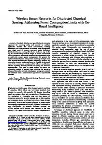
the 1- or 2-hop neighborhood depending on the version being considered. Iterating through every column of this matrix and adding every covering sensor to all existing covers allows us to construct all combinations of covers for the targets being considered. The covers obtained in this fashion form the nodes of the LD graph at that sensor. Associated with each cover is a lifetime given by the minimum energy sensor of that cover. This forms the node weight of the LD graph. To allow easy construction of edges for the LD graph we implement the covers as sets and their intersection represents the edges. In order to compare the algorithm against LBP and DEEPS, we use the same experimental setup as employed in [4]. We conduct the simulation with 25 targets randomly deployed, and vary the number of sensors between 40 and 120 with an increment of 20 and each sensor has a maximum sensing range (diameter) of 60m. The energy consumption model is linear. The results are shown in Figure 4. As can be seen from the figure, both the basic 1-hop and 2-hop algorithms outperform LBP. The 1-hop algorithm is almost as good as the 2-hop DEEPS algorithm. 50

Lifetime

40 LBP DEEPS

30

1-hop 2-hop

20

10 40

50

60

70

80

90

100

110

120

No. Of Sensors

Fig. 4. Network Lifetime for 25 targets with linear energy model

To study variations in targets and energy models, we simulate a network of 60 sensors with 60 m sensing range for both 25 and 50 targets and linear and quadratic energy models. The results are presented in Figure 5. We see a trend consistent with the previous plot with LBP being outperformed by the 1-hop and 2-hop algorithms and DEEPS and the 1-hop version showing similar lifetimes.

Lifetime

30 25

LBP

20

DEEPS

15

1-Hop

10

2-Hop

5 0 25 Targets, Linear

50 Targets, Linear

25 Targets, Quadratic

Fig. 5. Lifetime for 60 sensors with varying energy model and targets

390

S.K. Prasad and A. Dhawan

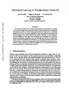
Fig. 6. Performance of Variants of the Basic Algorithm: Network Lifetime for 60 sensors, 25 targets, linear energy model

Finally, we simulate the different variants of the basic algorithm as outlined in Section III for a network of 60 sensors, 25 targets and a linear energy model. The results are shown in Figure 6 below. For the sake of comparison, we include the basic 1-hop and 2-hop algorithms in this plot also. We compare the 1-hop algorithm and its three variants against LBP. The percentage improvement for each algorithm against LBP is indicated on top of the bars. Similarly, we compare the 2-hop algorithm and Variant 4 against DEEPS. Overall improvements are in the 11-19% range.

5 Comparison with Existing Algorithms In this section we look at the existing approaches to solving the target coverage problem in a distributed fashion. In addition to the distributed algorithms, centralized approaches to the problem have also been considered in [2] [3]. An initial study of the coverage problem with disjoint cover sets was carried out in [10]. [2, 3] have a linear programming based solution that assigns a schedule that covers all targets while attempting to maximize the network lifetime. A related problem has been studied in [12] in which the authors present a power aware distributed algorithm to construct a connected dominating set. The work is an extension of [11] which presents simple localized rules to allow the distributed construction of a CDS. The CDS provides the network with connectivity in addition to coverage. We now focus on two existing approaches LBP[2] and DEEPS[4], show how they operate on an example topology and then present their equivalent representation in the lifetime dependency model. Load balancing protocol (LBP): LBP is a simple 1-hop protocol which works by attempting to balance the load between sensors. Sensors can be in one of three states sense/on, sleep/off or vulnerable/undecided. Initially all sensors are vulnerable and broadcast their battery levels along with information on which targets they cover. Based on this, a sensor decides to switch to off state if its targets are covered by a higher energy sensor in either on or vulnerable state. On the other hand, it remains on if it is the sole sensor covering a target.

Distributed Algorithms for Lifetime of Wireless Sensor Networks

391

Thus, LBP is simplistic and attempts to share the load evenly between sensors instead of balancing the energy for sensors covering a specific target. Hence, for the example shown in Figure 1, LBP picks the sensor s1 to be active since it is the largest sensor covering the bottom-left target T2. Similarly, it picks s2 for the bottom-right target T3. This results in a total lifetime of 3 units when compared to the optimal of 6 units for the given example. Its schedule is ({ s1, s2}, 3). Formulation using LD graph framework: LBP can be simulated as a special case in the lifetime dependency graph model as follows. Given a sensor si, its local covers for its targets T(si) are the singleton sets {s}, for all s ∈ N(si,1). These singleton sets are then assigned priorities in order to choose which one to use next. There are two defaults: the priority is highest if si is the only one covering a target (so si must switch on). On the other hand, the priority is lowest if all of si’s targets are covered, so that si can switch off. Otherwise, the priority is assigned based on the battery level preferring to burn those sensors with higher battery, with preference for those covers not containing si. Thus, a key limitation of LBP is the lack of collective negotiation captured by non-singleton cover sets in our algorithms. DEEPS protocol: The maximum duration that a target can be covered, its ‘life,’ is the sum of the batteries of all its nearby sensors that can cover it. The main intuition behind DEEPS is to try to minimize the energy consumption rate around those targets with smaller lives. A sensor thus has several targets with varying lives. A target is defined as a ‘sink’ if it is the shortest-life target for at least one sensor covering that target. Otherwise, it is a ‘hill.’ To guard against leaving a target uncovered during a shuffle, each target is assigned an in-charge sensor. For each sink, its in-charge sensor is the one with the largest battery for which this is the shortest-life target. For a hill target, its in-charge is that neighboring sensor whose shortest-life target has the longest life. An in-charge sensor does not switch off unless its targets are covered by someone. Apart from this, the rules are identical as those in LBP protocol. DEEPS relies on two-hop information to make these decisions. For the example shown in Figure 1, DEEPS achieves a lifetime of 5, assuming a shuffle round duration of 1 since initially both the sensors s1and s2 are switched on. Its schedule would be {{( s1, s2),1}, {( s1, s6),1}, {( s1, s7),1}, {( s2, s3), 1}, {( s2, s4),1}} for a total of 5 units. Formulation using LD graph framework: DEEPS can also be represented with our lifetime dependency graph model. The representation is just like LBP with singleton set covers from N(si ,1). The priority function of LBP is now modified suitably to account for the concept of in-charge sensors. Specifically, the order of priority preference is if a sensor alone can cover a target, a sensor is in-charge of a target, and then higher battery level. The default least priority is for a sensor if the target it is in-charge of is now covered. Again, singleton cover sets of DEEPS, as in LBP is its key limitation.

6 Conclusion This paper takes a fundamental look into the problem structure of finding longest lifetime schedule for covering targets by an ad-hoc wireless sensor network. The

392

S.K. Prasad and A. Dhawan

existing approaches typically employ greedy approaches based on sensor vs. its neighbors in trying to decide which sensors should be sensing and which ones can be in energy-conserving sleep mode. We consider the covers consisting of subsets of a sensor and its neighbors, which can cover all the nearby targets as a primary construct to decide the local on/off configuration of each neighborhood. The dependencies among the covers are modeled using a graph structure over the covers. The priority of a cover is a function of how minimally connected a cover is in this graph. This yields a basic framework, leading to several variants, with superior performance as compared to the existing distributed algorithms. The framework nature is further reinforced by demonstrating how other algorithms can be formulated. This work has opened up a new way to explore this problem. Even though the number of covers that each sensor transitions through is a function of the number of local neighbors and targets, both expected to be small, a more computationally efficient technique would be desirable. Several other variants of the basic framework are being explored.

References [1] Akyildiz, I.F., Su, W., Sankarasubramaniam, Y., Cayirci, E.: A Survey on Sensor Networks. In: IEEE Communications Magazine, pp. 102–114 (2002) [2] Berman, P., Calinescu, G., Shah, C., Zelikovsky, A.: Power Efficient Monitoring Management in Sensor Networks. In: IEEE Wireless Communication and Networking Conference (WCNC 2004), Atlanta, pp. 2329–2334 (March 2004) [3] Berman, P., Calinescu, G., Shah, C., Zelikovsky, A.: Efficient Energy Management in Sensor Networks. In: Xiao, Y., Pan, Y. (eds.) Ad Hoc and Sensor Networks, Wireless Networks and Mobile Computing, vol. 2, Nova Science Publishers (2005) [4] Brinza, D., Zelikovsky, A.: DEEPS: Deterministic Energy-Efficient Protocol for Sensor networks. In: ACIS International Workshop on Self-Assembling Wireless Networks (SAWN 2006) Proc. of SNPD, pp. 261–266 (2006) [5] Cardei, M., Thai, M.T., Li, Y., Wu, W.: Energy-efficient target coverage in wireless sensor networks. In: Proc. of IEEE Infocom (2005) [6] Cardei, M., Du, D.-Z.: Improving Wireless Sensor Network Lifetime through Power Aware Organization. ACM Wireless Networks 11(3) (May 2005) [7] Chong, C.-Y., Kumar, S.P.: Sensor Networks: Evolution, Opportunities and Challenges. Proceeding of the IEEE 91(8) (August 2003) [8] Garey, M.R, Johnson, D.S.: Computers and Intractability: A Guide to the Theory of NPCompleteness. W.H. Freeman, New York (1979) [9] Kumar, S., Lai, T.H., Balogh, J.: On k-coverage in a mostly sleeping sensor network. In: Proceedings of the 10th annual international conference on Mobile computing and networking, Philadelphia, PA, USA (2004) [10] Slijepcevic, S., Potkonjak, M.: Power efficient organization of wireless sensor networks. In: Proc. IEEE International Conference on Communications (ICC), pp. 472–476 (2001) [11] Li, W.: On calculating connected dominating set for efficient routing in ad hoc wireless networks. In: Proceedings of the 3rd international workshop on Discrete algorithms and methods for mobile computing and communications, pp. 7–14 (1999) [12] Wu, J., Dai, F., Gao, M., Stojmenovic, I.: On Calculating Power-Aware Connected Dominating Sets for Efficient Routing in Ad Hoc Wireless Networks. Journal of Communications and Networks 4(1) (March 2002)