Dynamic Graph Convolutional Networks Franco Manessi1 , Alessandro Rozza1 , and Mario Manzo2 1
arXiv:1704.06199v1 [cs.LG] 20 Apr 2017
2
Research Team - Waynaut {name.surname}@waynaut.com Servizi IT - Universit` a degli Studi di Napoli “Parthenope”
[email protected]
Abstract Many different classification tasks need to manage structured data, which are usually modeled as graphs. Moreover, these graphs can be dynamic, meaning that the vertices/edges of each graph may change during time. Our goal is to jointly exploit structured data and temporal information through the use of a neural network model. To the best of our knowledge, this task has not been addressed using these kind of architectures. For this reason, we propose two novel approaches, which combine Long Short-Term Memory networks and Graph Convolutional Networks to learn long short-term dependencies together with graph structure. The quality of our methods is confirmed by the promising results achieved.
1
Introduction
In machine learning, data are usually described as points in a vector space (x ∈ Rd ). Nowadays, structured data are ubiquitous and the capability to capture the structural relationships among the points can be particularly useful to improve the effectiveness of the models learned on them. To this aim, graphs are widely employed to represent this kind of information in terms of nodes/vertices and edges including the local and spatial information arising from data. Consider a d-dimensional dataset X = {x1 , . . . , xn } ⊂ Rd , the graph is extracted from X by considering each point as a node and computing the edge weights by means of a function. We obtain a new data representation G = (V, E), where V is a set, which contains vertices, and E is a set of weighted pairs of vertices (edges). Applications to a graph domain can be usually divided into two main categories, called vertex-focused and graph-focused applications. For simplicity of exposition, we just consider the classification problem.3 Under this setting, the vertex-focused applications are characterized by a set of labels L = {1, . . . , k}, a dataset X = {x1 , . . . , xl , xl+1 , . . . , xn } ⊂ Rd , the related graph G, and we assume that the first l points xi (where 1 ≤ i ≤ l) are labeled and the remaining xu (where l + 1 ≤ u ≤ n) are unlabeled. The goal is to classify the unlabeled nodes exploiting the combination of their features and the graph structure by 3
Notice that, the proposed formulation can be trivially rewritten for the regression problem.
2
means of a semi-supervised learning approach. Instead, graph-focused applications are related to the goal of learning a function f that maps different graphs to integer values by taking into account the features of the nodes of each graph: f (G i , X i ) ∈ L. This task can usually be solved using a supervised classification approach on the graph structures. A number of research works are devoted to classify structured data both for vertex-focused and graph-focused applications [9,19,21,23]. Nevertheless, there is a major limitation in existing studies, most of these research works are focused on static graphs. However, many real-world structured data are dynamic and nodes/edges in the graphs may change during time. In such dynamic scenario, temporal information can also play an important role. In the last decade, (deep) neural networks have shown their great power and flexibility by learning to represent the world as a nested hierarchy of concepts, achieving outstanding results in many different fields of application. It is important to underline that, just a few research works have been devoted to encode the graph structure directly using a neural network model [1,3,4,12,15,20]. Among them, to the best of our knowledge, no one is able to manage dynamic graphs. To exploit both structured data and temporal information through the use of a neural network model, we propose two novel approaches that combine Long Short Term-Memory networks (LSTMs, [8]) and Graph Convolutional Networks (GCNs, [12]). Both of them are able to deal with vertex-focused applications. These techniques are respectively able to capture temporal information and to properly manage structured data. Furthermore, we have also extended our approaches to deal with graph-focused applications. LSTMs are a special kind of Recurrent Neural Networks (RNNs, [10]), which are able to improve the learning of long short-term dependencies. All RNNs have the form of a chain of repeating modules of neural networks. Precisely, RNNs are artificial neural networks where connections among units form a directed cycle. This creates an internal state of the network which allows it to exhibit dynamic temporal behavior. In standard RNNs, the repeating module is based on a simple structure, such as a single (hyperbolic tangent) unit. LSTMs extend the repeating module by combining four interacting units. GCN is a neural network model that directly encodes graph structure, which is trained on a supervised target loss for all the nodes with labels. This approach is able to distribute the gradient information from the supervised loss and to enable it to learn representations exploiting both labeled and unlabeled nodes, thus achieving state-of-the-art results. The paper is organized as follows: in Section 2 the most related methods are summarized. In Section 3 we describe our approaches. In Section 4 a comparison with baseline methodologies is presented. Section 5 closes the paper by discussing our findings and potential future extensions.
3
2
Related Work
Many important real-world datasets are in graph form; among all, it is enough to consider: knowledge graphs, social networks, protein-interaction networks, and the World Wide Web. To deal with this kind of data achieving good classification results, the traditional approaches proposed in literature mainly follow two different directions: to identify structural properties as features to manage them using traditional learning methods, or to propagate the labels to obtain a direct classification. Zhu et al. [24] propose a semi-supervised learning algorithm based on a Gaussian random field model (also known as Label Propagation). The learning problem is formulated as Gaussian random fields on graphs, where a field is described in terms of harmonic functions, and is efficiently solved using matrix methods or belief propagation. Xu et al. [21] present a semi-supervised factor graph model that is able to exploit the relationships among nodes. In this approach, each vertex is modeled as a variable node and the various relationships are modeled as factor nodes. Grover and Leskovec, in [6], present an efficient and scalable algorithm for feature learning in networks that optimizes a novel network-aware, neighborhood preserving objective function using Stochastic Gradient Descent. Perozzi et al. [18] propose an approach called DeepWalk. This technique uses truncated random walks to efficiently learn representations for vertices in graphs. These latent representations, which encode graph relations in a vector space, can be easily exploited by statistical models thus producing state-of-the-art results. Unfortunately, the described techniques are not able to deal with graphs that dynamically change in time (nodes/edges in the graphs may change during time). There is a small amount of methodologies that have been designed to classify nodes in dynamic networks [14,22]. Li et al. [14] propose an approach that is able to learn the latent feature representation and to capture the dynamic patterns. Yao et al. [22] present a Support Vector Machines-based approach that combines the support vectors of the previous temporal instant with the current training data to exploit temporal relationships. Pei et al. [17] define an approach called dynamic Factor Graph Model for node classification in dynamic social networks. More precisely, this approach organizes the dynamic graph data in a sequence of graphs. Three types of factors, called node factor, correlation factor and dynamic factor, are designed to respectively capture node features, node correlations and temporal correlations. Node factor and correlation factor are designed to capture the global and local properties of the graph structures while the dynamic factor exploits the temporal information. It is important to underline that, very little attention has been devoted to the generalization of neural network models to structured datasets. In the last couple of years, a number of research works have revisited the problem of generalizing neural networks to work on arbitrarily structured graphs [1,3,4,12,15,20], some of them achieving promising results in domains that have been previously dominated by other techniques. Scarselli et al. [20] formalize a novel neural network model, called Graph Neural Network (GNNs). This model is based on extending a neural network method with the purpose of processing data in form of graph
4
structures. The GNNs model can process different types of graphs (e.g., acyclic, cyclic, directed, and undirected) and it maps a graph and its nodes into a Ddimensional Euclidean space to learn the final classification/regression model. Li et al. [15] extend the GNN model, by relaxing the contractivity requirement of the propagation step through the use of Gated Recurrent Unit [2], and by predicting sequence of outputs from a single input graph. Bruna et al. [1] describe two generalizations of Convolutional Neural Networks (CNNs, [5]). Precisely, the authors propose two variants: one based on a hierarchical clustering of the domain and another based on the spectrum of the Laplacian graph. Duvenaud et al. [4] present another variant of CNNs working on graph structures. This model allows an end-to-end learning on graphs of arbitrary size and shape. Defferrard et al. [3] introduce a formulation of CNNs in the context of spectral graph theory. The model provides efficient numerical schemes to design fast localized convolutional filters on graphs. It is important to notice that, it reaches the same computational complexity of classical CNNs working on any graph structure. Kipf and Welling [12] propose an approach for semi-supervised learning on graph-structured data (GCNs) based on CNNs. In their work, they exploit a localized first-order approximation of the spectral graph convolutions framework [7]. Their model linearly scales in the number of graph edges and learns hidden layer representations encoding local and structural graph features. Notice that, these neural network architectures are not able to properly deal with temporal information.
3
Our Approaches
In this section, we introduce two novel network architectures to deal with vertex /graph-focused applications. Both of them rely on the following intuitions: – GCNs can effectively deal with graph-structured information, but they lack the ability to handle data structures that change during time. This limitation is (at least) twofold: (i) inability to manage dynamic vertex features, (ii) inability to manage dynamic edge connections. – LSTMs excel in finding long short-term dependencies, but they lack the ability to explicitly exploit graph-structured information within it. Due to the dynamic nature of the tasks we are interested in solving, the new network architectures proposed in this paper will work on ordered sequences of graphs and ordered sequences of vertex features. Notice that, for sequences of length one, this reduces to the vertex/graph-focused applications described in Section 1. Our contributions are based on the idea of combining an extension of the Graph Convolution (GC, the fundamental layer of the GCNs) and a modified version of LSTM, thus to learn the downstream recurrent units by exploiting both graph structured data and vertex features. We propose two GC-like layers that take as input a graph sequence and the corresponding ordered sequence of vertex features, and they output an ordered sequence of a new vertex representation. These layers are:
5
– the Waterfall Dynamic-GC layer, which performs at each step of the sequence a graph convolution on the vertex input sequence. An important feature of this layer is that the trainable parameters of each graph convolution are shared among the various step of the sequence; – the Concatenate Dynamic-GC layer, which performs at each step of the sequence a graph convolution on the vertex input features, and concatenates it to the input. Again, the trainable parameters are shared among the steps in the sequence. Each of the two layers can jointly be used with a modified version of LSTM to perform a semi-supervised classification of sequence of vertices or a supervised classification of sequence of graphs. The difference between the two tasks just consists in how we perform the last processing of the data (for further details, see Equation (1) and Equation (2)). In the following section we will provide the mathematical definitions of the two modified GC layers, the modified version of LSTM, as well as some other handy definitions that will be useful when we will describe the final network architectures. 3.1
Definitions
Let (G i )i∈ZT with ZT := {1, 2, . . . , T } be a finite sequence of undirected graphs G i = (V i , E i ), with V i = V ∀i ∈ ZT , i.e. all the graphs in the sequence share the same vertices. Considering the graph G i , for each vertex v k ∈ V let xki ∈ Rd be the corresponding feature vector. Each step i in the sequence ZT can completely be defined by its graph G i (modeled by the adjacency matrix4 Ai ) and by the vertex-features matrix Xi ∈ R|V|×d (the matrix whose row vectors are the xki ). We will denote with [Y ]i,j the i-th row, j-th column element of the matrix Y , and with Y 0 the transpose of Y . Id is the identity matrix of Rd ; softmax and ReLU are the soft-maximum and the rectified linear unit functions [5]. The matrix P ∈ Rd×d is a projector on Rd if it is a symmetric, positive semi-definite matrix with P 2 = P . In particular, it is a diagonal projector if it is a diagonal matrix (with possibly some zero entries on the main diagonal). In other words, a diagonal projector on Rd is diagonal matrix with some 1s on the main diagonal, that when it is right-multiplied by a d-dimensional column vector v it zeroes out all the entries of v corresponding to the zeros on the main diagonal of P : P
v
Pv
1000 a a 0 0 0 0 b 0 0 0 1 0 c = c . 0001 d d We recall here the mathematics of the GC layer [12] and the LSTM [8], since they are the basic building blocks of our contribution. Given a graph with adjacency 4
Notice that, the adjacency matrices can be either weighted or unweighted.
6
matrix A ∈ R|V|×|V| and vertex-feature matrix X ∈ R|V|×d , the GC layer with M output nodes is defined as the function GCM : R|V|×d × R|V|×|V| → R|V|×M , ˆ such that GCM (X, A) := ReLU(AXB), where B ∈ Rd×M is a weight matrix ˆ is the re-normalized adjacency matrix, i.e. A ˆ := D ˜ -1/2 A ˜D ˜ -1/2 with A ˜ := and A P ˜ kk := ˜ kl . A + I|V| and [D] [ A] l Given the sequence (xi )i∈ZT with xi d-dimensional row vectors for each i ∈ ZT , a returning sequence-LSTM with N output nodes, is the function LSTMN : (xi )i∈ZT 7→ (hi )i∈ZT , with hi ∈ RN and hi = oi tanh(ci ), ci = ji cei + fi ci−1 , oi = σ(xi Wo + hi−1 Uo + bo ),
fi = σ(xi Wf + hi−1 Uf + bf ), ji = σ(xi Wj + hi−1 Uj + bj ), cei = σ(xi Wc + hi−1 Uc + bc ),
where is the Hadamard product, σ(x) := 1/(1 + e-x ), Wl ∈ Rd×N , Ul ∈ RN ×N are weight matrices and bl are bias vectors, with l ∈ {o, f, j, c}. Definition 1 (wd-GC layer). Let (Ai )i∈ZT , (Xi )i∈ZT be, respectively, the sequence of adjacency matrices and the sequence of vertex-feature matrices for the considered graph sequence (G i )i∈ZT , with Ai ∈ R|V|×|V| and Xi ∈ R|V|×d ∀i ∈ ZT . The Waterfall Dynamic-GC layer with M output nodes is the function wd-GCM with weight matrix B ∈ Rd×M defined as follows: ˆi Xi B) )i∈Z wd-GCM : ((Xi )i∈ZT , (Ai )i∈ZT ) 7→ ( ReLU(A T ˆi Xi B) ∈ R|V|×M , and all the A ˆi are the re-normalized adjacency where ReLU(A matrices of the graph sequence (G i )i∈ZT . The wd-GC layer can be seen as multiple copies of a standard GC layer, all of them sharing the same training weights. Then, the resulting training parameters are d · M , independently of the length of the sequence. In order to introduce the Concatenate Dynamic-GC layer, we recall the definition of the Graph of a Function: considering a function f from A to B, [GF f ] : A → A × B, x 7→ [GF f ](x) := (x, f (x)). Namely, the GF operator transforms f into a function returning the concatenation between x and f (x). Definition 2 (cd-GC layer). Let (Ai )i∈ZT , (Xi )i∈ZT be, respectively, the sequence of adjacency matrices and the sequence of vertex-feature matrices for the considered graph sequence (G i )i∈ZT , with Ai ∈ R|V|×|V| and Xi ∈ R|V|×d ∀i ∈ ZT . A Concatenate Dynamic-GC layer with M output nodes is the function cd-GCM with weight matrix B ∈ Rd×M defined as follows: ˆi Xi B) )i∈Z cd-GCM : ((Xi )i∈ZT , (Ai )i∈ZT ) 7→ ( [GF ReLU](A T ˆi Xi B) ∈ R|V|×(M +d) , and all the A ˆi are the re-normalized where [GF ReLU](A adjacency matrices of the graph sequence (G i )i∈ZT .
7
Intuitively, cd-GC is a layer made of T copies of GC layers, each copy acting on a specific instant of the sequence. Each output of the T copies is then concatenated with its input, thus resulting in a sequence of graph-convoluted features together with the vertex-features matrix. Note that, the weights B are shared among the T copies. The number of learnable parameters of this layer is d · (d + M ), independently of the number of steps in the sequence (G i )i∈ZT . Notice that, both the input and the output of wd-GC and cd-GC are sequences of matrices (loosely speaking, third order tensors). We will now define three additional layers. These will help us in reducing the clutter with the notation when we will introduce in Section 3.2 and Section 3.3 the network architectures we have used to solve the semi-supervised classification of sequence of vertices and the supervised classification of sequence of graphs. Precisely, they are: (i) the recurrent layer used to process in a parallel fashion the convoluted vertex features, (ii) the two final layers (one per task) used to map the previous layers outputs into k-class probability vectors. Definition 3 (v-LSTM layer). Consider (Zi )i∈ZT with Z ∈ RL×M , the Vertex LSTM layer with N output nodes is given by the function v-LSTMN : LSTMN ((V10 Zi )i∈ZT ) .. L×N ×T , v-LSTMN : (Zi )i∈ZT 7→ ∈R . LSTMN ((VL0 Zi )i∈ZT )
where Vp is the isometric embedding of R into RL defined as [Vp ]i,j = δip , and δ is the Kronecker delta function. The training weights are shared among the L copies of the LSTMs. Definition 4 (vs-FC layer). Consider (Zi )i∈ZT with Z ∈ RL×N , the Vertex Sequential Fully Connected layer with k output nodes is given by the function vs-FCk , parameterized by the weight matrix W ∈ RN ×k and the bias matrix 0 RL×k 3 B := (b0 , . . . , b0 ) : vs-FCk : (Zi )i∈ZT 7→ ( softmax(W Zi + B) )i∈ZT with softmax(W Zi + B) ∈ RL×k . Definition 5 (gs-FC layer). Consider (Zi )i∈ZT with Z ∈ RL×N , the Graph Sequential Fully Connected layer with k output nodes is given by the function gs-FCk , parameterized by the weight matrices W1 ∈ RN ×k , W2 ∈ R1×L and the 0 bias matrices RL×k 3 B1 := (b0 , . . . , b0 ) and B2 ∈ R1×k : gs-FCK : (Zi )i∈ZT 7→ ( softmax(W2 ReLU(W1 Zi + B1 ) + B2 ) )i∈ZT with softmax(W2 ReLU(W1 Zi + B1 ) + B2 ) ∈ R1×k . Informally: (i) the v-LSTM layer acts as L copies of LSTM, each one evaluating the sequence of one row of the input tensor (Zi )i∈ZT ; (ii) the vs-FC layer acts as T copies of a Fully Connected layer (FC, [5]) with softmax activation, all the copies
8 Instant 4 Instant 3 Instant 2 Instant 1 Vertex 1
x11
Vertex 2
x12
Vertex 3
x13
Vertex 4
x14
A1
GC
LSTM LSTM LSTM LSTM LSTM
FC FC FC FC FC FC
wd-GC
v-LSTM
gs-FC
x15
Vertex 5
Vertex-features Adjacency matrices matrices
z1
Graph predictions
(a) WD-GCN for classification of sequence of graphs. Instant 4 Instant 3 Instant 2 Instant 1 Vertex 1
x11
Vertex 2
x12
Vertex 3
x13
Vertex 4
x14
Vertex 5
x15
A1
Vertex-features Adjacency matrices matrices
GC cd-GC
LSTM LSTM LSTM LSTM LSTM
FC FC FC FC FC
v-LSTM
vs-FC
[Z1]1,: [Z1]1,: [Z1]1,: [Z1]1,: [Z1]1,: Vertices predictions
(b) CD-GCN for classification of sequence of vertices.
Figure 1: The figure shows two of the four network architectures presented in Sections 3.2 and 3.3, both of them working on sequences of four graphs composed of five vertices, i.e. (G i )i∈Z4 , |V| = 5. (a) The wd-GC layer acts as four copies of a regular GC layer, each one working on an instant of the sequence. The output of this first layer is processed by the v-LSTM layer that acts as five copies of the returning sequence-LSTM layer, each one working on a vertex of the graphs. The final gs-FC layer, which produces the k-class probability vector for each instant of the sequence, can be seen as the composition of two layers: the first one working on each vertex for every instant, and the following one working on all the vertices at a specific instant. (b) The cd-GC and the v-LSTM layers work as the wd-GC and the v-LSTM of the Figure 1a, the only difference is that v-LSTM works both on graph convolutional features, as well as plain vertex features, due to the fact that cd-GC produces their concatenation. The last layer, which produces the k-class probability vector for each vertex and for each instant of the sequence, can be seen as 5 × 4 copies of a FC layer.
sharing the parameters. The vs-FC layer outputs L k-class probability vectors for each step in the input sequence; (iii) the gs-FC layer acts as T copies of two FC layers with softmax-ReLU activation, all the copies sharing the parameters. This layer outputs one k-class probability vector for each step in the input sequence. Note that, both the input and the output of vs-FC and v-LSTM are sequences of matrices, while for gs-FC the input is a sequence of matrices and the output is a sequence of vectors. We have now all the elements to describe our network architectures to address both semi-supervised classification of sequence of vertices and supervised classification of sequence of graphs.
9
3.2
Semi-Supervised Classification of Sequence of Vertices
Definition 6 (Semi-Supervised Classification of Sequence of Vertices). Let (G i )i∈ZT be a sequence of T graphs each one made of |V| vertices, and (Xi )i∈ZT the related sequence of vertex-features matrices. Let (PiLab )i∈ZT be a sequence of diagonal projectors on the vector space R|V| . Define the sequence (PiUnlab )i∈ZT by means of PiUnlab := I|V| − PiLab , ∀i ∈ ZT ; i.e. PiLab and PiUnlab identify the labeled and unlabeled vertices of G i , respectively. Moreover, let (Yi )i∈ZT be a sequence of T matrices with |V| rows and k columns, satisfying the property PiLab Yi = Yi , where the j-th row of the i-th matrix represents the one-hot encoding of the k-class label of the j-th vertex of the i-th graph in the sequence, with the j-th vertex being a labeled one. Then, semisupervised classification of sequence of vertices consists in learning a function f such that PjLab f ( (G i )i∈ZT , (Xi )i∈ZT )j = Yj and PjUnlab f ( (G i )i∈ZT , (Xi )i∈ZT )j is the right labeling for the unlabeled vertices for each j ∈ ZT . To address the above task, we propose the networks defined by the following functions: v wd-GC LSTMM,N,k : v cd-GC LSTMM,N,k :
vs-FCk ◦ v-LSTMN ◦ wd-GCM ,
(1a)
vs-FCk ◦ v-LSTMN ◦ cd-GCM ,
(1b)
where ◦ denote the function composition. Both the architectures take ((Xi )i∈ZT , (Ai )i∈ZT ) as input, and produce a sequence of matrices whose row vectors are the probabilities of each vertex of the graph: (Zi )i∈ZT with Zi ∈ R|V|×k . For the sake of clarity, in the rest of the paper, we will refer to the networks defined by Equation (1a) and Equation (1b) as Waterfall Dynamic-GCN (WD-GCN) and Concatenate Dynamic-GCN (CD-GCN, see Figure 1b), respectively. Since all the functions involved in the composition are differentiable, the weights of the architectures can be learned using gradient descent methods, employing as loss function the cross-entropy evaluated only on the labeled vertices: L=−
X X X
[Yt ]v,c log[PtLab Zt ]v,c ,
t∈ZT c∈Zk v∈Z|V|
with the convention that 0 · log 0 = 0. 3.3
Supervised Classification of Sequence of Graphs
Definition 7 (Supervised Classification of Sequence of Graphs). Let (G i )i∈ZT be a sequence of T graphs each one made of |V| vertices, and (Xi )i∈ZT the related sequence of vertex-features matrices. Moreover, let (yi )i∈ZT be a sequence of T one-hot encoded k-class labels, i.e. yi ∈ {0, 1}k . Then, graphsequence classification task consists in learning a predictive function f such that f ( (G i )i∈ZT , (Xi )i∈ZT ) = (yi )i∈ZT .
10
The proposed architectures are defined by the following functions: g wd-GC LSTMM,N,k :
gs-FCk ◦ v-LSTMN ◦ wd-GCM ,
(2a)
g cd-GC LSTMM,N,k :
gs-FCk ◦ v-LSTMN ◦ cd-GCM ,
(2b)
The two architectures take as input ((Xi )i∈ZT , (Ai )i∈ZT ). The output of wd-GC and cd-GC is processed by a v-LSTM, resulting in a |V| × N matrix for each step in the sequence. It is a gs-FC duty to transform this vertex-based prediction into a graph based prediction, i.e. to output a sequence of k-class probability vectors (zi )i∈ZT . Again, we will use WD-GCN (see Figure 1a) and CD-GCN to refer to the networks defined by Equation (2a) and Equation (2b), respectively. Also under this setting the training can be performed by means of gradient descent methods, with the cross entropy as loss function: X X L=− [yt ]c log[zt ]c , t∈ZT c∈Zk
with the convention 0 · log 0 = 0.
4
Experimental Results
In this section we describe the employed datasets, the experimental settings, and the results achieved by our approaches compared with those obtained by baseline methods. 4.1
Datasets
We now present the used datasets. The first one is employed to evaluate our approaches in the context of the vertex-focused applications; instead, the second dataset is used to assess our architectures in the context of the graph-focused applications. Our first set of data is a subset of DBLP5 dataset described in [17]. Conferences from six research communities, including artificial intelligence and machine learning, algorithm and theory, database, data mining, computer vision, and information retrieval, have been considered. Precisely, the co-author relationships from 2001 to 2010 are considered and data of each year is organized in a graph form. Each author represents a node in the network and an edge between two nodes exists if two authors have collaborated on a paper in the considered year. Note that, the resulting adjacency matrix is unweighted. The node features are extracted from each temporal instant using DeepWalk [18] and are composed of 64 values. Furthermore, we have augmented the node features by adding the number of articles published by the authors in each of the six communities, obtaining a features vector composed of 70 values. This specific task belongs to the vertex-focused applications. 5
http://dblp.uni-trier.de/xml/
11
The original dataset is made of 25.215 authors across the ten years under analysis. Each year 4.786 authors appear on average, and 114 authors appear all the years, with an average of 1.594 authors appearing on two consecutive years. We have considered the 500 authors with the highest number of connections during the analyzed 10 years, i.e. the 500 vertices among the total 25.215 with P P the highest t∈Z10 i [At ]i,j , with At the adjacency matrix at the t-th year. If one of the 500 selected authors does not appear in the t-th year, its feature vector is set to zero. The final dataset is composed of 10 vertex-features matrices in R500×70 , 10 adjacency matrices belonging to R500×500 , and each vertex belongs to one of the 6 classes. CAD-1206 is a dataset composed of 122 RGB-D videos corresponding to 10 high-level human activities [13]. Each video is annotated with sub-activity labels, object affordance labels, tracked human skeleton joints and tracked object bounding boxes. The 10 sub-activity labels are: reaching, moving, pouring, eating, drinking, opening, placing, closing, scrubbing, null. Our second dataset is composed of all the data related to the detection of sub-activities, i.e. no object affordance data have been considered. Notice that, detecting the sub-activities is a challenging problem as it involves complex interactions, since humans can interact with multiple objects during a single activity. This specific task belongs to the graph-focused applications. Each one of the 10 high-level activities is characterized by one person, whose 15 joints are tracked (in position and orientation) in the 3D space for each frame of the sequence. Moreover, in each high-level activity appears a variable number of objects, for which are registered their bounding boxes in the video frame together with the transformation matrix matching extracted SIFT features [16] from the frame to the ones of the previous frame. Furthermore, there are 19 objects involved in the videos. We have built a graph for each video frame: the vertices are the 15 skeleton joints plus the 19 objects, while the weighted adjacency matrix has been derived by employing Euclidean distance. Precisely, among two skeleton joints the edge weight is given by the Euclidean distance between their 3D positions; among two objects it is the 2D distance between the centroids of their bounding boxes; among an object and a skeleton joint it is the 2D distance between the centroid of the object bounding box and the skeleton joint projection into the 2D video frame. All the distances have been scaled between zero and one. When an object does not appear in a frame, its related row and column in the adjacency matrix is set to zero. Since the videos have different lengths, we have padded all the sequences to match the longest one, which has 1.298 frames. Finally, the feature columns have been standardized. The resulting dataset is composed of 122×1.298 vertex-feature matrices belonging to R34×24 , 122×1.298 adjacency matrices (in R34×34 ), and each graph belongs to one of the 10 classes. 6
http://pr.cs.cornell.edu/humanactivities/data.php
12
4.2
Experimental Settings
In our experiments, we have compared the results achieved by the proposed architectures with those obtained by other baseline networks (see Section 4.3 for a full description of the chosen baselines). For the baselines that are not able to explicitly exploit sequentiality in the data, we have flatten the temporal dimension of all the sequences, thus considering the same point in two different time instants as two different training samples. The hyper-parameters of all the networks (in terms of number of nodes of each layer and dropout rate) have been appropriately tuned by means of a grid approach. The performances are assessed employing 10 iterations of Monte Carlo Cross-Validation7 preserving the percentage of samples for each class. It is important to underline that, the 10 train/test sets are generated once, and they are used to evaluate all the architectures, to keep the experiments as fair as possible. To assess the performances of all the considered architectures we have employed Accuracy and Unweighted F1 Measure 8 . Moreover, the training phase has been performed using Adam [11] for a maximum of 100 epochs, and for each network (independently for Accuracy and F1 Measure) we have selected the epoch where the learned model achieved the best performance on the validation set using the learned model to finally assess the performance on the test set. 4.3
Results
DBLP We have compared the approaches proposed in Section 3.2 (WD-GCN and CD-GCN) against the following baseline methodologies: (i) a GCN composed of two layers, (ii) a network made of two FC layers, (iii) a network composed of LSTM+FC, (iv) and a deeper architecture made of FC+LSTM+FC. Note that, the FC is a Fully Connected layer; when it appears as the first layer of a network it employes a ReLU activation, instead a softmax activation is used when it is the last layer of a network. The test set contains 30% of the 500 vertices. Moreover, 20% of the remaining vertices (the training ones) have been used for validation purposes. It is important to underline that, an unlabeled vertex remains unlabeled for all the years in the sequence, i.e. considering Definition 6, PiLab = P Lab , ∀i ∈ ZT . In Table 1, the best hyper-parameter configurations together with the test results of all the evaluated architectures are presented. 7
8
This approach randomly selects (without replacement) some fraction of the data to build the training set, and it assignes the rest of the samples to the test set. This process is repeated multiple times, generating (at random) new training and test partitions each time. Notice that, in our experiments, the training set is further split into training and validation. The Unweighted F1 Measure the F1 scores for each label class, and find P evaluates c rc their unweighted mean: k1 c∈Zk p2p , where pc and rc are the precision and the +r c c recall of the class c.
13
Table 1: Results of the evaluated architectures on semi-supervised classification of sequence of vertices employing the DBLP dataset. We have tested the statistical significance of our result by means of Wilcoxon test, obtaining a p-value < 0.6% when we have compared WD-GCN and CD-GCN against all the baselines for both the employed scores. Accuracy Best Performance Config. mean ± std
Unweighted F1 Measure Best Performance Config. mean ± std
1st FC nodes: {150, 200, 250, 300, 350, 400} {0%, 10%, 20%, 30%, 40%, 50%} dropout:
250 50%
49.1% ± 1.2%
250 40%
48.2% ± 1.3%
GC+GC
1st GC nodes: {150, 200, 250, 300, 350, 400} {0%, 10%, 20%, 30%, 40%, 50%} dropout:
350 50%
54.8% ± 1.4%
350 10%
54.7% ± 1.7%
LSTM+FC
LSTM nodes: dropout:
{100, 150, 200, 300, 400} {0%, 10%, 20%, 30%, 40%, 50%}
100 0%
60.1% ± 2.1%
100 0%
60.4% ± 2.3%
FC nodes: FC+LSTM+FC LSTM nodes: dropout:
{100, 200, 300, 400} {100, 200, 300, 400} {0%, 10%, 20%, 30%, 40%, 50%}
300 300 50%
61.8% ± 1.9%
300 300 50%
61.8% ± 2.4%
WD-GCN
wd-GC nodes: {100, 200, 300, 400} v-LSTM nodes: {100, 200, 300, 400} dropout: {0%, 10%, 20%, 30%, 40%, 50%}
300 300 50%
70.0% ± 3.0%
400 300 0%
70.7% ± 2.4%
CD-GCN
cd-GC nodes: {100, 200, 300, 400} v-LSTM nodes: {100, 200, 300, 400} dropout: {0%, 10%, 20%, 30%, 40%, 50%}
200 100 50%
70.1% ± 2.8%
200 100 50%
70.5% ± 2.7%
Network
Hyper-params Grid
FC+FC
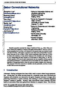
Employing the best configuration for each of the architectures in Table 1, we have further assessed the quality of the tested approaches by evaluating them by changing the ratio of the labeled vertices as follows: 20%, 30%, 40%, 50%, 60%, 70%, 80%. To obtain robust estimations, we have averaged the performances by means of 10 iterations of Monte Carlo Cross-Validation. Figure 2 reports the results of this experiment. Both the proposed architectures have obtained promising results that have overcome those achieved by the considered baselines. Moreover, we have shown that the WD-GCN and the CD-GCN performances are roughly equivalent in terms of Accuracy and Unweighted F1 Measure. Architectures such as GCNs and LSTMs are mostly likely limited for their inability to exploit jointly graph structure and long short-term dependencies. Note that, the structure of the graphs appearing in the sequence is not exclusively conveyed by the DeepWalk vertex-features, and it is effectively captured by the GC units. Indeed, the two layers-GCN has obtained better results with respect to those achieved by the two FC layers. It is important to underline that, the WD-GCN and the CD-GCN have achieved better performances with respect to the baselines not for the reason they exploit a greater number of parameters, or since they are deeper, rather: – the baseline architectures have achieved their best performances without employing the maximum amount of allowed number of nodes, thus showing that their performance is unlikely to become better with an even greater number of nodes; – the number of parameters of our approaches is significatly lower than the number of parameters of the biggest employed network: i.e. the best WD-GCN
14
(a) Accuracy.
(b) Unweighted F1 Measure.
Figure 2: The figure shows the performances of the tested approaches (on the DBLP dataset) varying the ratio of the labeled vertices. The vertical bars represent the standard deviation of the performances achieved in the 10 iterations of the Monte Carlo cross-validation.
and CD-GCN have, respectively, 872.206 and 163.406 parameters, while the largest tested network is the FC+LSTM+FC with 1.314.006 parameters; – the FC+LSTM+FC network has a comparable depth with respect to our approaches, but it has achieved lower performance. Finally, WD-GCN and CD-GCN have shown little sensitivity to the labeling ratio, further demonstrating the robustness of our methods. CAD-120 We have compared the approaches proposed in Section 3.3 against a GC+gs-FC network, a vs-FC+gs-FC architecture, a v-LSTM+gs-FC network, and a deeper architecture made of vs-FC+v-LSTM+gs-FC. Notice that, for this architectures, the vs-FCs are used with a ReLU activation, instead of a softmax. The 10% of the videos has been selected for testing the performances of the model, and 10% of the remaining videos has been employed for validation. Table 2 shows the results of this experiment. The obtained results have shown that only CD-GCN has outperformed the baseline, while WD-GCN has reached performances similar to those obtained by the baseline architectures. This difference may be due to the low number of vertices in the sequence of graphs. Under this setting, the predictive power of the graph convolutional features is less effective, and the CD-GCN approach, which augments the plain vertex-features with the graph convolutional ones, provides an advantage. Hence, we can further suppose that, while WD-GCN and CD-GCN are suitable to effectively exploit structure in graphs with high vertex-cardinality, only the latter can deal with dataset with limited amount of nodes. It is worth noting that, despite all the experiments have shown a high variance in their performances, the Wilcoxon test has shown that CD-GCN is statistically better than the baselines with a p-value < 5% for the Unweighted F1 Measure and < 10% for the Accuracy. This reveals that in almost
15
Table 2: Results of the evaluated architectures on supervised classification of sequence of graphs employing the CAD-120 dataset. CD-GCN is the only technique comparing favourably to all the baselines, resulting in a Wilcoxon test with a p-value lower than 5% for the Unweighted F1 Measure and lower than 10% for the Accuracy. Accuracy Best Performance Config. mean ± std
Unweighted F1 Measure Best Performance Config. mean ± std
1st vs-FC nodes: {100, 200, 250, 300} {0%, 20%, 30%, 50%} dropout:
100 20%
49.9% ± 5.2%
200 20%
48.1% ± 7.2%
GC+gs-FC
1st GC nodes: dropout:
{100, 200, 250, 300} {0%, 20%, 30%, 50%}
250 30%
46.2% ± 3.0%
250 50%
36.7% ± 7.9%
v-LSTM+gs-FC
LSTM nodes: dropout:
{100, 150, 200, 300} {0%, 20%, 30%, 50%}
150 0%
56.8% ± 4.1%
150 0%
53.0% ± 9.9%
vs-FC nodes: vs-FC+v-LSTM+gs-FC v-LSTM nodes: dropout:
{100, 200, 250, 300} {100, 150, 200, 300} {0%, 20%, 30%, 50%}
200 150 20%
58.7% ± 1.5%
200 150 20%
57.5% ± 2.9%
WD-GCN
wd-GC nodes: v-LSTM nodes: dropout:
{100, 200, 250, 300} {100, 150, 200, 300} {0%, 20%, 30%, 50%}
250 150 30%
54.3% ± 2.6%
250 150 30%
50.6% ± 6.3%
CD-GCN
cd-GC nodes: v-LSTM nodes: dropout:
{100, 200, 250, 300} {100, 150, 200, 300} {0%, 20%, 30%, 50%}
250 150 30%
60.7% ± 8.6%
250 150 30%
61.0% ± 5.3%
Network
Hyper-params
vs-FC+gs-FC
Grid
every iteration of the Monte Carlo Cross-Validation, the CD-GCN has performed better than the baselines. Finally, the same considerations presented for the DBLP dataset regarding the depth and the number of parameters are valid also for this set of data.
5
Conclusions and Future Works
We have introduced for the first time, two neural network approaches that are able to deal with semi-supervised classification of sequence of vertices and supervised classification of sequence of graphs. Our models are based on modified GC layers connected with a modified version of LSTM. We have assessed their performances on two datasets against some baselines, showing the superiority of both of them for semi-supervised classification of sequence of vertices, and the superiority of CD-GCN for supervised classification of sequence of graphs. We can hypothesize that the differences between the WD-GCN and the CD-GCN performances when the graph size is small are due to the feature augmentation approach employed by CD-GCN. This conjecture should be addressed in future works. In our opinion, interesting extensions of our work may consist in: (i) the usage of alternative recurrent units to replace LSTM; (ii) to propose further extensions of the GC unit; (iii) to explore the performance of deeper architectures that combine the layers proposed in this work.
16
References 1. Bruna, J., Zaremba, W., Szlam, A., LeCun, Y.: Spectral networks and locally connected networks on graphs. In: ICLR (2013) 2. Cho, K., van Merri¨enboer, B., G¨ ul¸cehre, C ¸ ., Bahdanau, D., Bougares, F., Schwenk, H., Bengio, Y.: Learning phrase representations using RNN encoder–decoder for statistical machine translation. In: EMNLP. pp. 1724–1734 (2014) 3. Defferrard, M., Bresson, X., Vandergheynst, P.: Convolutional neural networks on graphs with fast localized spectral filtering. In: NIPS (2016) 4. Duvenaud, D.K., Maclaurin, D., Iparraguirre, J., Bombarell, R., Hirzel, T., AspuruGuzik, A., Adams, R.P.: Convolutional networks on graphs for learning molecular fingerprints. In: NIPS (2015) 5. Goodfellow, I., Bengio, Y., Courville, A.: Deep Learning. MIT Press (2016) 6. Grover, A., Leskovec, J.: Node2vec: Scalable feature learning for networks. In: ACM SIGKDD. pp. 855–864. ACM (2016) 7. Hammond, D.K., Vandergheynst, P., Gribonval, R.: Wavelets on graphs via spectral graph theory. Applied and Comput. Harmonic Analysis 30 (2), 129–150 (2011) 8. Hochreiter, S., Schmidhuber, J.: Long short-term memory. Neural Comput. 9(8), 1735–1780 (Nov 1997) 9. Jain, A., Zamir, A.R., Savarese, S., Saxena, A.: Structural-RNN: Deep learning on spatio-temporal graphs. In: CVPR. pp. 5308–5317. IEEE (2016) 10. Jain, L.C., Medsker, L.R.: Recurrent Neural Networks: Design and Applications. CRC Press, Inc., 1st edn. (1999) 11. Kingma, D., Ba, J.: Adam: A method for stochastic optimization. In: ICLR (2015) 12. Kipf, T.N., Welling, M.: Semi-supervised classification with graph convolutional networks. In: ICLR (2017) 13. Koppula, H.S., Gupta, R., Saxena, A.: Learning human activities and object affordances from RGB-D videos. Int. J. Rob. Res. 32(8), 951–970 (Jul 2013) 14. Li, K., Guo, S., Du, N., Gao, J., Zhang, A.: Learning, analyzing and predicting object roles on dynamic networks. In: IEEE ICDM. pp. 428–437 (2013) 15. Li, Y., Tarlow, D., Brockschmidt, M., Zemel, R.S.: Gated graph sequence neural networks. In: ICLR (2016) 16. Lowe, D.G.: Object recognition from local scale-invariant features. In: ICCV. pp. 1150–1157. IEEE (1999) 17. Pei, Y., Zhang, J., Fletcher, G.H., Pechenizkiy, M.: Node classification in dynamic social networks. In: AALTD 2016: 2nd ECML-PKDD International Workshop on Advanced Analytics and Learning on Temporal Data. pp. 54–93 (2016) 18. Perozzi, B., Al-Rfou, R., Skiena, S.: Deepwalk: Online learning of social representations. In: ACM SIGKDD. pp. 701–710. ACM (2014) 19. Rozza, A., Manzo, M., Petrosino, A.: A novel graph-based fisher kernel method for semi-supervised learning. In: ICPR. pp. 3786–3791. IEEE (2014) 20. Scarselli, F., Gori, M., Tsoi, A.C., Hagenbuchner, M., Monfardini, G.: The graph neural network model. IEEE Trans. Neural Networks 20(1), 61–80 (2009) 21. Xu, H., Yang, Y., Wang, L., Liu, W.: Node classification in social network via a factor graph model. In: PAKDD. pp. 213–224 (2013) 22. Yao, Y., Holder, L.: Scalable SVM-based classification in dynamic graphs. In: IEEE ICDM. pp. 650–659 (2014) 23. Zhao, Y., Wang, G., Yu, P.S., Liu, S., Zhang, S.: Inferring social roles and statuses in social networks. In: ACM SIGKDD. pp. 695–703. ACM (2013) 24. Zhu, X., Ghahramani, Z., Lafferty, J., et al.: Semi-supervised learning using gaussian fields and harmonic functions. In: ICML. vol. 3, pp. 912–919 (2003)