namic models, but this chapter uses “dynamic process models” as a ... niques of
model-based data analysis, model-targeted experimentation and model-.
3
1
Dynamic Process Modeling: Combining Models and Experimental Data to Solve Industrial Problems Mark Matzopoulos
Keywords steady-state modeling, first-principles modeling, dynamic modeling, high fidelity modeling, Fischer–Tropsch reaction, model-based engineering (MBE), parameter estimation, computation fluid dynamic (CFD) model 1.1 Introduction
The operation of all processes varies over time. Sometimes this is an inherent part of the process design, as in batch processes or pressure swing adsorption; sometimes it is as a result of external disturbances, for example a change in feedstock or product grade, equipment failure, or regular operational changes such as the diurnal load variation of a power plant or the summer–winter operation of a refinery. Many processes are intended to run and indeed appear to run at steady state, and for practical purposes of design they can be modeled as such. However for inherently dynamic processes, or when considering transient aspects of otherwise “steady-state” processes – for example, start-up, shutdown, depressurization, and so on – steady-state or pseudo-steady-state analysis is simply not applicable, or is at best a gross simplification. Such cases require dynamic process models. By modeling the time-varying aspects of operation we are not simply “adding another dimension” to steady-state models. There are many factors that, when considered as a whole, represent a step change beyond the philosophy and approach taken in traditional steady-state modeling. There are of course many different levels of fidelity possible when creating dynamic models, but this chapter uses “dynamic process models” as a shorthand for high-fidelity predictive process models (which generally include dynamics) that typically combine chemical engineering first principles theory with observed, “reallife” data. It looks at how these can be systematically applied to complex problems within industry to provide value in a whole range of process systems. At the heart of the approaches described here is a family of methodologies that use models to perform many different tasks: not only to simulate and optimize process performance but also to estimate the parameters used in the equations Process Systems Engineering: Vol. 7 Dynamic Process Modeling Edited by Michael C. Georgiadis, Julio R. Banga, and Efstratios N. Pistikopoulos Copyright © 2011 WILEY-VCH Verlag GmbH & Co. KGaA, Weinheim ISBN: 978-3-527-31696-0
4
1 Dynamic Process Modeling: Combining Models and Experimental Data to Solve Industrial Problems
on which those simulations and optimizations are based; to analyze experimental data and even to design the experiments themselves. The methodologies also make it possible to move from relatively little experimental data collected in small-scale equipment to a high-fidelity predictive model of a complex and large-scale industrial unit or process. As these methodologies are underpinned by a mathematical model, or series of mathematical models, they are known as model-based methodologies – in particular model-based engineering and model-based innovation and their supporting techniques of model-based data analysis, model-targeted experimentation and modelbased experiment design. This chapter describes how these techniques can be systematically applied to create models that are capable of predicting behavior over a wide range of conditions and scales of operation with unprecedented accuracy. 1.1.1 Mathematical Formulation
Process systems are often most readily specified in terms of a mixed set of integral, partial differential and algebraic equations, or IPDAEs, and this is the chosen representation of most established software designed specifically for process systems engineering. Traditionally, IPDAE systems are reduced into a mixed set of ordinary differential and algebraic equations, or DAEs. While ordinary differential equations (ODEs) typically arise from the conservation of fundamental quantities of nature, algebraic equations (AEs) result from processes where accumulation is not important or transients are considered to occur instantaneously, as well as by introduction of auxiliary relationships among variables. Discontinuities in the governing phenomena of physical, chemical, and biological systems frequently arise from thermodynamic, transport, and flow transitions as well as structural changes in the control configuration. While some of these transitions are intrinsically reversible and symmetric discontinuities, others are reversible and asymmetric or irreversible discontinuities. State-of-the-art languages incorporate powerful mechanisms to declare any type of transitions (for example, if-then-else and case constructs) which can be nested to an arbitrary depth. A second class of discontinuities arises from external actions imposed by the surroundings on the system at a particular point in time, typically discrete manipulations and disturbances such as operating procedure or imposed failures. The ability to incorporate complex sets of discontinuities describing a series of states in the formulation of a DAE system leads to the concept of state-task networks (STNs) [1]. Many, though not all, modern custom-modeling tools are capable of solving complex problems involving arbitrarily complex combinations of DAE and STN systems. In this chapter we are not concerned with the mathematics of dynamic modeling; this is well covered in the literature. The focus is rather on the practical and systematic application of the high-fidelity process models, using now well-established principles of model-based engineering, to add value to industrial operations.
1.2 Dynamic Process Modeling – Background and Basics
1.1.2 Modeling Software
Custom-modeling tools based on general-purpose, high-level, equation-oriented, declarative modeling languages are becoming the standard tools of the trade for the development and application of high-fidelity predictive models, particularly when full control over the scope and detail of the process model is required [2]. Such tools can support many of the activities essential for the effective dynamic process modeling that is the subject of this volume. Established commercial examples of general-purpose custom-modeling platforms for integrated simulation and optimization (including in some cases model validation and design activities) include Aspen Technology’s Aspen Custom Modeler® , Process Systems Enterprise’s gPROMS® and Dassault Systèmes’s Dymola® ; open source initiatives include EMSO (Environment for Modeling, Simulation and Optimization) and Open Modelica.
1.2 Dynamic Process Modeling – Background and Basics
The state-of-the-art in process modeling has moved well beyond the “material and energy accounting” exercises of steady-state flowsheeting applications (which nevertheless still represent a large proportion of process modeling activity) to become a central platform for capture and deployment of companies’ Intellectual Property (IP). A systematic modeling activity using high-fidelity predictive models provides a set of tools that enables companies to adapt – rapidly if necessary – to changing market drivers and gain competitive advantage. Models, if properly constructed, embody valuable corporate knowledge in such a way that it can be rapidly accessed and deployed to generate immediate commercial value. For example, during an economic downturn the models originally used to optimize equipment design can be rapidly redeployed with a different objective: reducing operating cost. For example, a model may be used to capture the definitive set of reaction kinetic relationships that may represent many years’ worth of experimentation. This reaction network model can then be used as part of a reactor model to redesign the reaction process, or to adapt an operating process to improve its economics under new market conditions. The knowledge developed during the redesign or adaptation – for example, regarding the performance of alternative reactor internal configurations or catalyst formulations – is often valuable information in itself. This new information can be captured in the model for use in future analysis, or to form the basis of patent applications in support of licensed process development, and so on. It is possible in this way to enter a virtuous cycle where each use of the model generates information that increases its usefulness in the future; every subsequent activity increases the return on initial modeling investment.
5
6
1 Dynamic Process Modeling: Combining Models and Experimental Data to Solve Industrial Problems
1.2.1 Predictive Process Models
In order to describe modeling approach and practice, it is worth first defining what we mean by a “process model.” For the purposes of this chapter a process model is considered to be a set of mathematical relationships and data that describe the behavior of a process system, capable of being implemented within a process modeling environment in such a way that they can be used to generate further knowledge about that system through simulation, optimization, and other related activities. To be more specific, a chemical engineering model – whether written in a programming language such as Fortran or C or a modern modeling language such as gPROMS language or Modelica – is typically a collection of physics, chemistry, engineering, operating and economic knowledge in equation form, coupled in some way with empirically determined data. To be useful in design and operational analysis, a model should have a predictive capability so that given, for example, a new set of feed or operating conditions or design parameters, it calculates accurate revised rates for the output values of interest. At its best, a model is capable of predicting actual behavior with accuracy over a wide range of conditions without refitting the model parameters, making it possible to explore the design or operational space consistently and comprehensively and be confident in the results. In order to be predictive, a model needs to take into account all the phenomena that significantly affect the output values of interest, to the required degree of accuracy. For example, a model that includes a very detailed reaction kinetic representation but ignores diffusion effects for a reaction that is severely diffusion-limited will not provide very useful results. Conversely there is little point in including detailed intrapore diffusion effects in a catalytic reaction model when it is known that reactions are fast and occur largely on the catalyst surface; the unnecessary detail may increase calculation times and reduce model robustness for very little gain in accuracy. Generally, current practice is to construct “fit-for-purpose” models wherever the modeling software environment allows this; in many cases these can be “parameterized” in order easily to include or exclude phenomena. 1.2.2 Dynamic Process Modeling
Most process engineers are familiar with steady-state simulation modeling from some stage of their careers, typically in the form of widely available process flowsheeting packages such as Aspen Technology’s AspenPlusTM and Hysys® , and Invensys Process Systems’ PRO/II® . The key ostensible difference between the steady-state models of these packages and dynamic process models is the ability to take into account variation over time. However, as can be seen below the difference is not simply the addition of a time dimension; dynamic modeling often brings a whole different approach that results
1.2 Dynamic Process Modeling – Background and Basics
in dynamic models being a much truer-to-life representation of the process in many other respects. While steady-state analysis is mainly used for process flowsheet design, usually to determine mass and energy balances and approximate equipment sizes, or perhaps stream properties, the ability of dynamic models to model transient behavior opens up a whole new world of application. Typical applications of dynamic models are as follows:
• • • • • • • • • • •
analysis of transient behavior, including performance during start-up, shutdown, and load change; regulatory (i.e., PID) control scheme analysis and design; design of optimal operating procedures – for example, to optimize transition between product grades; design of batch processes; design of inherently dynamic continuous processes – for example, pressure swing adsorption; fitting data from nonsteady-state operations – for example, dynamic experiments, which contain much more information than steady-state experiments, or estimation of process parameters from transient plant data; safety analysis – for example, the determination of peak pressures on compressor trip; inventory accounting and reconciliation of plant data; online or offline parameter re-estimation to determine key operating parameters such as fouling or deactivation constants; online soft-sensing; operator training.
1.2.3 Key Considerations for Dynamic Process Models
There are of course many different types of dynamic model, from simple transferfunction models often used for control system design, through operator training simulation models and “design simulators” to fully fledged process models containing a high-fidelity representation of physics and chemistry and capable of being solved in a number of different ways. Here we are more interested in the latter end of this range. In a dynamic model the simple assumptions of a steady-state model – for example, that material always flows from an upstream unit where the pressure is higher to a lower pressure downstream pressure unit – may no longer be valid. Transients in the system may cause the “downstream” pressure to become higher than the “upstream” pressure, causing flow reversal; the model has to allow for this possibility. This requirement for a “pressure-driven” approach is just one example. There are many others: the following are some of the considerations that need to be taken into account in a reliable dynamic process model:
7
8
1 Dynamic Process Modeling: Combining Models and Experimental Data to Solve Industrial Problems
•
•
•
•
•
•
Material transport. Material cannot simply be assumed to flow from one unit to another conveniently in “streams.” The device in which it is transported (typically a pipe) itself needs to be treated as a piece of equipment and modeled. Flow – and the direction of flow – is determined by pressure gradients and resistance considerations, which may be different depending on the direction of flow, as well as flow regime. Flow reversal. As mentioned above, it is necessary to provide appropriate mechanisms for reverse flow into units where there is material accumulation. It is also necessary to provide for the fact that the intrinsic properties (for example, specific enthalpy) of the stream change when flow is reversed to correspond to the properties of the material leaving the downstream, rather than the upstream, unit. This requires proper definition of streams at the downstream boundary of the flowsheet to include reverse-flow “inlet” properties. Equipment geometry. The physical geometry of equipment may have a significant effect on the dynamics, and needs to be taken into account. For example, the time dynamics of a distillation column depend on the tray area, weir height, bubble cap vapor flow area, and so on. Not only do the spatial relationships need to be represented in the model, but also a whole additional category of data – typically taken from design specification sheets – is required. Process control and control devices. In steady-state modeling, as the term implies, state variables (typically those representing accumulation of mass and energy, or their close relatives such as level, temperature, and pressure) can simply be set to the required values as required. In dynamic models, as in real life, these values vary as a result of external influences – for example, pressure or level is affected by the changing flowrates in and out of a vessel – and cannot be set. As on the physical plant, the states need to be maintained at their “set point” values through the use of controllers and associated measurement and control devices. These devices need to be represented fully in the dynamic model. Phase disappearance. During transient behavior phases may appear and disappear. For example, a flash drum that would normally operate in a vapor–liquid two-phase region may generate liquid only if the pressure rises above the bubblepoint pressure or the temperature drops below the bubble-point temperature. The transition between phase regimes is very challenging numerically and the solution engine needs to be able to handle the calculation robustly and efficiently. Equilibrium. In general, steady-state simulators assume equilibrium between phases, for example, in distillation calculations. During transient situations operation may depart significantly from equilibrium and mass transfer limitations become important. The assumption of equilibrium between phases can no longer be taken for granted, and rate-based mass transfer modeling is required (note that rate-based considerations can be equally important in a steady-state representation).
There are other areas where representation tends to be (or in many cases, needs to be) much more accurate in dynamic models than steady-state models – for example, in representation of reaction kinetics.
1.2 Dynamic Process Modeling – Background and Basics
The proper inclusion of the phenomena listed above results in a significant enhancement in fidelity of representation and range of applicability over and above that afforded by the simple addition of accumulation terms. The inclusion of these phenomena not only requires greater modeling effort; it also requires an appreciation of the structural consistency issues resulting from inclusion of many closely interrelated effects. When specifying the set or assigned variable values for a dynamic simulation, for example, it is generally necessary to specify quantities that would be fixed or considered constant in real-life operation, such as equipment dimensions, controller set points, and upstream and downstream boundary conditions. Also, in some cases the “simplifying assumptions” used in steady-state models (for example, constant holdups on distillation trays) lead to a high-index dynamic problem [3]; resolving this may take considerable additional modeling effort. Choosing a consistent set of initial conditions, and providing meaningful numerical values for these variables, is not a trivial undertaking for those coming from a steady-state modeling paradigm. Many modelers struggle with this task which, though not complex, nevertheless requires attention, knowledge, and additional modeling effort. The remainder of this chapter takes “dynamic process models” as a shorthand for high-fidelity predictive models that embody many or all of the representations described above. 1.2.4 Modeling of Operating Procedures
A significant and important advantage of dynamic process modeling is the ability to model – and hence optimize – operating procedures, including production recipes, simultaneously with equipment and process. The ability to optimize operating procedures is of course an essential requirement in the design of batch process systems. However, it also has significant application to continuous processes. For example, it is possible to model process start-up procedure as a series of tasks (“start pump P102, continue until level in vessel L101 is 70%, open steam valve CV113, . . . ,” etc.), each of which may involve executing a set of defined subtasks. Given a suitably detailed start-up procedure and a model that is capable of providing accurate results (and executing robustly) over the range of operating conditions encountered – which may include significant nonequilibrium operation – it is possible not only to simulate the plant behavior during start-up but also to optimize the start-up sequence. The objective function in such cases is usually economic – for example, “start-up to on-spec production in the minimum time/at the lowest cost.” Constraints are typically rate limitations or material limits – for example, “subject to a maximum steam rate of x kg/s,” “subject to the temperature in vessel L141 never exceeding y degrees C,” etc.
9
10
1 Dynamic Process Modeling: Combining Models and Experimental Data to Solve Industrial Problems
Other applications are in the design and optimization of feedstock or product grade change procedures for complex processes. Many hours of off-spec production can often be eliminated by using dynamic optimization to determine the optimal process variable trajectories to maximize a profit objective function. 1.2.5 Key Modeling Concepts
There are a number of key terms and concepts that frequently arise in any discussion on high-fidelity predictive modeling that are worth touching on briefly. 1.2.5.1 First-Principles Modeling For the purposes of this discussion, the term first-principles modeling is intended to reflect current generally accepted chemical engineering first-principles representation of natural phenomena derived from the conservation of mass, energy, and momentum. More specifically, this implies material and energy balances, hydraulic relationships, multicomponent diffusion, reaction kinetic relationships, material properties as provided by typical physical property packages, and so on, all applied to distinct physical components or pseudocomponents – rather than first-principles representation at a submolecular level. While there are emerging techniques that will allow incorporation of molecular-level representation within process models, allowing simultaneous design of molecule and process [4], for the purposes of this chapter we assume the existence of predefined fixed molecules with known properties. 1.2.5.2 Multiscale Modeling In many chemical engineering problems important phenomena – i.e., those that have a significant effect on the behavior of a process – may occur at a number of different spatial and temporal scales. For example, the size of a slurry-bed reactor for Fischer–Tropsch gas-to-liquid conversion (typically tens of meters in height) is strongly influenced by the micronscale diffusion of reactants and product within catalyst particle pores. In order to successfully optimize the design of such a reactor, the model needs to represent key relationships and phenomena at both extremes as well as all the intermediate scales. If such a model is to be placed within a plant flowsheet, yet another scale needs to be taken into account. In some cases – for example, rate-based distillation – well-defined theoretical models exist [5] that take into account the relevant phenomena, from film diffusion to whole column operation. It is relatively straightforward to implement these within a modeling package. In others, the modeler needs to apply significant ingenuity to represent all the required scales within a computationally tractable solution. An example is a multitubular reactor model, where a full representation needs to couple an accurate shell-side fluid model with highly detailed models of the catalyst-filled tubes within the shell. The shell-side fluid model alone may require discretization (meshing)
1.2 Dynamic Process Modeling – Background and Basics
running to hundreds of thousands or even millions of cells. Tube models require at least a 2D representation (a third spatial dimension may be required to account for a distribution along the catalyst pore depth) in which the full reaction-withdiffusion model is solved at each grid point. There may be 20 000 such tubes in a multitubular reactor, each experiencing a different external temperature profile because of nonuniformity in the shell-side fluid flows at any given shell radius. In such a case a full representation of all scales would result in hundreds of millions of equations to be solved. This is obviously not a viable approach, and the model needs to be reduced in size significantly and in such a way that the accuracy is preserved. As software becomes more powerful, the challenge of representing different scales within a single model (or hierarchy of models) decreases; however, brute force is not necessarily the answer. There are numerous techniques and methodologies for reducing the computational effort required to deal with different scales, from the stepwise approach to parameter estimation at different scales described in Section 1.3.3 to the multizonal hybrid modeling approaches that couple the computational fluid dynamic (CFD) representation of hydrodynamics with phenomenological models of processes such as crystallization [6], to the interpolation techniques used to effect model reduction in fuel cell stacks. The example in Section 1.4 outlines a tractable approach for high-fidelity multitubular reactor modeling that is now applied routinely to provide accurate detailed design information. 1.2.5.3 Equation-Based Modeling Tools Past practice tended to combine models – the relationships describing a process – with their mathematical solution, often with data thrown into the mix in the form of hard-coded values or empirical functions with limited range of applicability. In many cases “black box” models, they were written in programming languages such as Fortran, DELPHI, or C, with users unable to modify or even see the underlying relationships. New unit models needed to be coded from scratch, including all their internal numerical solution code, which sometimes took months of effort. Such models were typically inflexible, limited in scope and predictive capability, capable of being solved in a single direction only, difficult to maintain, and often lacking in robustness. Modern “equation-based” or “equation-oriented” tools separate the engineering aspects from the mathematical solution using fourth-generation languages or graphical representations; good modeling practice ensures that model and data are separated too. This means that a complex unit can be now described in tens of lines of physics and chemistry relationships rather than thousands of lines of code required in the past, with significant implications for development time, quality assurance, ease of understanding and maintenance and re-usability – and of course lifecycle cost. This fact alone has removed significant hurdle from the development and application of models. The removal of the mathematics means that it is possible to extend the fidelity and range of application of models easily. For example, a lumped parameter
11
12
1 Dynamic Process Modeling: Combining Models and Experimental Data to Solve Industrial Problems
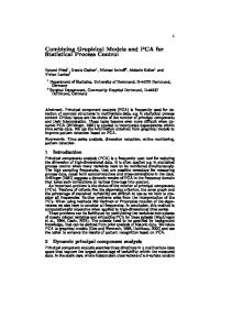
Fig. 1.1 A fixed-bed reactor model can involve a four-
dimensional distribution – for example, the four spatial and one property distribution shown here.
pipeline or heat exchanger model can be turned into a much more accurate distributed system model with a few days’ effort rather than months of programming. 1.2.5.4 Distributed Systems Modeling The more sophisticated equation-based custom-modeling environments make it possible to model distributions in size, space, or any other relevant quantity easily. Consider a fixed-bed Fischer–Tropsch tubular reaction process converting syngas into longer chain hydrocarbons (Fig. 1.1). Axial and radial distributions are used to represent the distribution of concentration, temperature, and other quantities along and across the tube. A further spatial distribution is used to representing changing conditions along the length of the catalyst pores (essential for this severely diffusion-limited reaction). Finally the bulk of the product from the Fischer–Tropsch reaction – longer chain hydrocarbons with various numbers of carbon atoms – is modeled as a distribution of carbon numbers. Without any one of these distributions the model would not be able to represent the system behavior accurately. Sophisticated tools go further, allowing for nonuniform grids. This can be important in reducing system size while maintaining accuracy. An example is the modeling of a catalyst tube in a highly exothermic reaction, where much of the action takes place close to the beginning of the active catalyst bed. In this area of steep gradients, it is desirable to have many discretization grid points; however, in the areas of relatively low reaction further down the tube having many points would simply result in unnecessary calculation. Some tools go further, providing adaptive grids that are capable of modeling moving-front reactions to high accuracy with a relatively small number of discretization points.
1.2 Dynamic Process Modeling – Background and Basics
1.2.5.5 Multiple Activities from the Same Model A key advantage of equation-based systems is that it is possible to perform a range of engineering activities with the same model. In other words, the same set of underlying equations representing the process can be solved in different ways to provide different results of interest to the engineer or researcher. Typical examples are:
• • •
•
•
•
Steady-state simulation: for example, given a set of inlet conditions and unit parameters, calculate the product stream values. Steady-state design: for example, given inlet and outlet values, solve the “inverse problem” – i.e., calculate equipment parameters such as reactor diameter. Steady-state optimization: vary a selected set of optimization variables (for example, unit parameters such as column diameter, feed tray location, or specified process variables such as cooling water temperature) to find the optimal value of a (typically economic) objective function, subject to constraints. Dynamic simulation: given a consistent set of boundary conditions (for example, upstream compositions and flowrates or pressure and downstream pressure, unit parameters and initial state values, show how the process behaves over time. Dynamic simulations typically include the control infrastructure as an integral part of the simulation. The process is typically subject to various disturbances; the purpose of the simulation is usually to gauge the effect of these disturbances on operation. Dynamic optimization: determine the values and/or trajectories of optimization variables that maximize or minimize a (typically economic) objective function, subject to constraints. Dynamic optimization is used, for example, to determine the optimal trajectories for key process variables during feedstock or product grade change operations in order to minimize off-spec production. It effectively removes the need to perform repeated trial-and-error dynamic simulations. Parameter estimation: fit model parameters to data using formal optimization techniques applied to a model of the experiment, and provide confidence information on the fitted parameters.
There are many other ways in which model can be used, for example, for sensitivity analysis, model-based experiment design, model-based data analysis, generation of linearized models for use in other contexts (for example, in control design or within model-based predictive controllers) and so on. 1.2.5.6 Simulation vs. Modeling It is useful at this point to distinguish between dynamic simulators or simulation tools and dynamic modeling tools. The former generally perform a single function only (in fact they are often limited by their architecture to doing this): the dynamic simulation activity described above. Frequently dynamic simulators cannot solve for steady state directly, but need to iterate to it. Operator training simulators are a typical example of dynamic simulators.
13
14
1 Dynamic Process Modeling: Combining Models and Experimental Data to Solve Industrial Problems
Fully featured dynamic process modeling tools can perform dynamic simulation as one of the set of possible model-based activities. They treat the model simply as a representation of the process in equation form, without prior assumption regarding how these equations will be solved.
1.3 A Model-Based Engineering Approach
As the term implies, a model-based engineering (MBE) approach involves performing engineering activities with the assistance of a mathematical model of the process under investigation. MBE applies high-fidelity predictive models in combination with observed (laboratory, pilot, or plant) data to the engineering process in order to explore the design space as fully and effectively as possible and support design and operating decisions. Typical application is in new process development or optimization of existing plants. Closely related is model-based innovation, where a similar approach is used at R&D level to bridge the gap between experimental programs and engineering design, and capture corporate knowledge in usable form, typically for early-stage process or product development. Key objectives of both approaches are to:
• • •
accelerate process or product innovation, by providing fast-track methods to explore the design space while reducing the need for physical testing; minimize (or effectively manage) technology risk by allowing full analysis of design and operational alternatives, and identifying areas of poor data accuracy; integrate R&D experimentation and engineering design in order to maximize effectiveness of both activities and save cost and time.
At the heart of the model-based engineering approach are high-fidelity predictive models that typically incorporate many of the attributes described in the previous section. 1.3.1 High-Fidelity Predictive Models
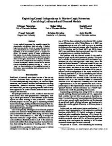
In order to create a high-fidelity predictive model it is necessary to combine theoretical knowledge and empirical information derived from real-world measurement (Fig. 1.2). Current best practice is to:
•
fix (in equation form) everything that can reliably be known from theory. Typically this involves writing equations for heat and material balance relationships, reaction kinetics, hydraulic relationships, geometry, etc., many of which are based on well-understood chemical engineering theory or can be found in model libraries or literature;
1.3 A Model-Based Engineering Approach
Fig. 1.2 The constituents of a high-fidelity predictive model:
first-principles theoretical relationships and real-world (laboratory, pilot or operating) data.
•
then estimate the empirical constants using the information already contained within the model in conjunction with experimental data.
The key objective is to arrive at a model that is accurately predictive over a range of scales and operating conditions. In order to do this it is necessary to include a representation of all the phenomena that will come into play at the scales and conditions for which the model will be executed, and to determine accurate scaleinvariant model parameters, where is possible. It is the combination of the first-principles theory and suitably refined data that provides the uniquely predictive capability of such models over a wide range of conditions. This approach brings the best of both worlds, combining as it does well-known theory with actual observed values. But how does is it implemented in practice? This is explored in the subsequent sections.
15
16
1 Dynamic Process Modeling: Combining Models and Experimental Data to Solve Industrial Problems
1.3.2 Model-Targeted Experimentation
Model-based engineering requires a different approach to experimentation from that traditionally employed. Traditionally experimentation is carried out in such a way that the results of the experiment can be used to optimize the process. For example, experiments are designed to maximize production of the main product rather than impurities; the knowledge gained from the experiment is used directly to attempt to maximize the production on the real plant. Model-targeted experimentation instead focuses on experiments that maximize the accuracy of the model. The model, not the experimental data, is then used to optimize the design. Model-targeted experimentation is just a likely to require an experiment that maximizes production of an impurity rather than the main product, in order to better characterize the kinetics of the side reaction. With accurate characterization of all key reactions it is possible accurately to predict the effect on product purity, for example, of minor changes in operating temperature. 1.3.3 Constructing High-Fidelity Predictive Models – A Step-by-Step Approach
Typically predictive models are constructed in a modular fashion in a number of steps, each of which may involve validation against laboratory or pilot plant experimental data. The validation steps will require a model of the process in which the experimental data is being collected – not a model of the full-scale equipment at this stage – that includes a description of the relevant phenomena occurring within that process. For example, consider the case where reaction data are being collected using a small-scale semibatch reactor with a fixed charge of catalyst, for the purposes of estimating reaction kinetic parameter values to be used in a reactor design. The model used for parameter estimation needs to provide a high-fidelity representation of the semibatch experimental process, as well as the rate equations proposed for the expected set of reactions and any diffusion, heat transfer or other relevant effects. If the model does not suitably represent what is occurring in the experiment, the mismatch will be manifest as uncertainty in the estimated parameter values; this uncertainty will propagate through the design process and eventually surface as a risk for the successful operation of the final design. The procedure below provides a condensed step-by-step approach to constructing a validated model of a full-scale process plant (Fig. 1.4). It assumes access to equation-based modeling software where it is possible to program first principles models and combine these in some hierarchical form in order to represent multiple scales, as well as into flowsheets in order to represent the broader process. It also assumes software with a parameter estimation capability.
1.3 A Model-Based Engineering Approach
The key steps in constructing a validated first-principles model with a good predictive capability over a range of scales are as follows: Step 1 – Construct the first-principles model This is probably perceived as the most daunting step for people not familiar with the art. However it need not be as onerous as it sounds. If starting from scratch, many of the relationships that need to be included have been known for generations: conservation of mass, conservation of momentum, conservation of energy and pressure-flow relationships are standard tools of the trade for chemical engineers. Thermophysical properties are widely available in the form of physprop packages, either commercially or in-house. Maxwell–Stefan multicomponent diffusion techniques, though complicated, are well-established and can provide a highly accurate representation of mass transfer with minimal empirical (property) data. Most researchers dealing with reaction have a fair idea of the reaction set and a reasonable intuition regarding which reactions are predominant. Molecular modeling research can provide guidance on surface reactions. If necessary, a reaction set and rate equations can be proposed then verified (or otherwise) using model-discrimination techniques based on parameter estimation against experimental data [7]. Of course it is not necessary to go to extremes of modeling every time. The challenge to the modeler often lies in selecting the appropriate level of fidelity for the requirements and availability of data – if a reaction is rate-limited rather than diffusion-limited it is not necessary to include diffusion relationships. Restricting the modeled relationships strictly to those required to obtain an accurate answer helps make the resulting mathematical problem more robust and faster to solve, but it does restrict generality. Having said that, most modelers do not start from scratch; there is an increasing body of first-principles models of many types of process available from university research, in equation form in the literature, or as commercially supplied libraries. Many first-principles models can be found in equation form with a careful literature search. An interesting tendency is that as models increasingly are constructed from faithful representations of fundamental phenomena such as multicomponent mass transfer and reaction kinetics, the core models become more universally applicable to diverse processes. For example, the core models used to represent the reaction and mass transfer phenomena in a reactive distillation provide essential components for a bubble column reactor model; similarly the multi-dimensional fixed-bed catalytic reactor models that take into account intrapore diffusion into catalyst particles provide most of a model framework required for a high-fidelity model of a pressure-swing adsorber. Organizations investing in constructing universally applicable first-principles models – as opposed to “shortcut” or empirical representations – are likely to reap the fruit of this investment many times over in the future.
17
18
1 Dynamic Process Modeling: Combining Models and Experimental Data to Solve Industrial Problems
Fig. 1.3 Fitting experimental data to a model of the experiment in order to generate model parameter values.
Step 2 – Estimate the model parameters from data Having constructed a first principles model, it will often be necessary – or desirable – to estimate some parameters from data. This is almost always the case when dealing with reaction, for example, where reaction kinetic parameters – virtually impossible to predict accurately based on theory – need to be inferred from experimental data. Other typical parameters are heat transfer coefficients, crystal growth kinetic parameters, and so on. Initial parameter values are usually taken from literature or corporate information sources as a starting point. Parameter estimation techniques use models of the experimental procedure within an optimization framework to fit parameter information to experimental data (Fig. 1.3). With modern techniques it is possible to estimate simultaneously large numbers of the parameters occurring in complex nonlinear models – involving tens or hundreds of thousands of equations – using measurements from any number of dynamic and/or steady-state experiments. Maximum likelihood techniques allow instrument and other errors inherent in practical experimentation to be taken directly into account, or indeed to be estimated simultaneously with the model parameter values. When dealing with a large number of parameters, parameters at different scales can be dealt with in sequential fashion rather than simultaneously. For example it is common practice to estimate reaction kinetics from small-scale (of the order
1.3 A Model-Based Engineering Approach
of centimeters) experiments in isothermal conditions, then maintain these parameters constant when fitting the results of subsequent larger scale experiments to measure “equipment” parameters such as catalytic bed heat transfer coefficients. Parameter estimation effectively “tunes” the model parameters to reflect the observed (“real-life”) behavior as closely as possible. If performed correctly, with data gathered under suitably defined and controlled conditions, estimation can generate sets of parameter that are virtually scale invariant. This has enormous benefits for predictive modeling used in design scale-up. It means that, for instance, the reaction kinetic or crystal growth parameters determined from experimental apparatus at a scale of cubic centimeters can accurately predict performance in equipment several orders of magnitude larger, providing that effects that become significant at larger scales – such as hydrodynamic (e.g., mixing) effects – are suitably accounted for in the model. Parameter estimation can be simpler or more challenging than it sounds, depending in the quantity and quality of data available. It is a process that often requires a significant amount of engineering judgment. Step 3 – Analyze the experimental data Parameter estimation has an important additional benefit: model-based data analysis. The estimation process produces quantitative measures of the degree of confidence associated with each estimated parameter value, as well as estimates of the error behavior of the measurement instruments. Confidence information is typically presented in the form of confidence ellipsoids. Often this analysis exposes inadequacies in the data – for example certain reaction kinetic constants in which there is a poor degree of confidence, or which are closely correlated with other parameters. In some cases parameters can exhibit poor confidence intervals even if the values predicted using the parameters appears to fit the experimental data well. Using model-based data analysis it is usually easy to identify the parameters of most concern and devise additional experiments that will significantly enhance the accuracy of – and confidence in – subsequent designs. Poor data can be linked to design and operational risk in a much more formal manner. Using techniques currently under development [8], global sensitivity analysis coupled with advanced optimization methods can be used to map the uncertainty in various parameters – in the form of probability distributions – onto the probability distributions for plant key performance indicators (KPIs). This translates the uncertainty inherent in, say, a reaction kinetic parameter, directly into a quantitative risk for the success of the plant performance. For example if the real parameter value turns out to be in a certain region within the confidence ellipsoid the designed plant may not make a profit, or may end up operating in an unsafe region. The ability to relate KPIs such as profit directly to parameter uncertainty through the medium of a high-fidelity predictive model means that often-scarce research funding can be directed into the study of the parameters that have the greatest
19
20
1 Dynamic Process Modeling: Combining Models and Experimental Data to Solve Industrial Problems
effect on these KPIs. This makes it possible to justify R&D spending based on a quantitative ranking. Step 4 – Design additional experiments, if necessary In some cases it will be obvious which additional experiments need to be carried out, and how they need to be carried out. For more complex situations, in particular cases where experiments are expensive or time consuming, there are benefits in applying more formal experiment design techniques. A major development in the last few years has been the emergence of modelbased techniques for the design of experiments [7]. In contrast to the usual statistically based techniques (e.g., factorial design), model-based experiment design takes advantage of the significant amount of information that is already available in the form of the mathematical model. This is used to design experiments which yield the maximum amount of parameter information, thereby minimizing the uncertainty in any parameters estimated from the results of these experiments. This optimization-based technique is applicable to the design of both steady-state and dynamic experiments, and can be applied sequentially taking account of any experiments that have already been performed. Figure 1.4 shows how model-based experiment design fits within the MBE procedure. Typical decision variables determined by model-based experiment design include the optimal conditions under which the new experiment is to be conducted (e.g., the temperature profile to be followed over the duration of the experiment), the optimal initial conditions (e.g., initial charges and temperature) and the optimal times at which measurements should be taken (e.g., sampling times for off-line analysis). The overall effect is that the required accuracy in the estimated parameter values may be achieved using the minimum number of experiments. In addition to maximizing the improvement in parameter accuracy per experiment, the approach typically results in significantly reduced experimentation time and cost. Steps 2 to 4 are repeated until parameter values are within acceptable accuracy. Determining “acceptable accuracy” in this context generally means evaluating the effects of possible values of parameters on key design criteria (for example, the conversion of a key component in a reactor) using the model, as part of a formal or informal risk assessment of the effect on plant KPIs. Generally, if any combination of the potential parameter values results in unacceptable predicted operation (for example, subspecification products or uneconomic operation) – even if other combinations demonstrate acceptable operation – the parameter values need to be refined by going around the experimentation cycle again. Steps 1 to 4 may also be repeated to develop submodels at different scales, covering different phenomena. Typically the parameters fitted during earlier analyses are held constant (i.e., considered to be fixed), providing in effect a “model reduction” for the parameter estimation problem by reducing the number of parameters to be fitted at each step and allowing the experiments at each step to focus on the phenomena of interest. The procedure at each stage is the same: build a model that contains the key phenomena, conduct experiments that generate the required
1.3 A Model-Based Engineering Approach
Fig. 1.4 Model-based engineering – a schematic overview of procedure and methodologies.
data as unambiguously as possible, estimate the relevant parameters, then “fix” this model and parameters in subsequent investigations at different scales. Step 5 – Build the process model Once the parameter confidence analysis indicates an acceptable margin of uncertainty in the parameters, the submodels can then be used in construction of the full equipment model. If necessary, this can be validated against operating or test run data to determine, for example, overall heat transfer or flow coefficients. It should not be necessary, and indeed would be counterproductive, to estimate parameters already fixed from the earlier laboratory or pilot validation at this stage. Building the full model typically involves assembling the relevant submodels of phenomena at different scales, defining appropriate boundary conditions (flows, pressures, stream and external wall temperatures, etc.) and if necessary including ancillary equipment such as heat exchangers, pumps and compressors, recycles, and so on within a flowsheet representation.
21
22
1 Dynamic Process Modeling: Combining Models and Experimental Data to Solve Industrial Problems
1.3.4 Incorporating Hydrodynamics Using Hybrid Modeling Techniques
When scaling up, or simply constructing models of larger-scale equipment, the assumption of perfect mixing may not hold. In such cases the model needs to take into account fluid dynamics in addition to the accurate representation of diffusion, reaction and other “process” phenomena. The IPDAE software modeling systems used for the process chemistry representation are not ideally suited for performing detailed hydrodynamic modeling of fluid behavior in irregular geometries. An approach that is increasingly being applied is to couple a computation fluid dynamic (CFD) model of the fluid dynamics to the process model in order to provide hydrodynamic information [6]. Such “hybrid modeling” applications fall into two broad classes: those where the CFD and process models model different aspects of the same volumes, and those where they model different volumes, sharing information at surface boundaries. Such linking of CFD models with models of process and chemistry is a wellestablished practice used for design of crystallizers, slurry-bed reactors, multitubular reactors, fuel cells, and many other items of equipment. In most cases the CFD model provides initial input values to the process model; these may be updated periodically based on information generated by the process model and provided back to the CFD model but in general intensive iteration between the two is (fortunately) not required. The combination makes available the best features of both modeling approaches. An example is crystallizer modeling, where each model represents different aspects of the same physical volume, usually a stirred vessel. The process model is divided into a number of well-mixed zones (typically between 5 and 50), each of which is mapped onto groups of cells in the CFD model. The CFD model calculates the velocity field, in particular the flows in and out of the zone, and may also provide turbulent dissipation energy information for the crystallization calculation. The process model performs the detailed crystallization population balance calculation for the zone, as well as calculating the kinetics of nucleation, growth, attrition and agglomeration and any other relevant phenomena, based on the information received from the CFD model. 1.3.5 Applying the High-Fidelity Predictive Model
If Steps 1 to 4 have been followed diligently and Step 5 model has been constructed with due care by taking into account all the relevant phenomena, the resulting model should be capable of predictive behavior over a wide range of scales and conditions. The model can now be used to optimize many different aspects of design and operation. It is possible to, for example:
1.4 An Example: Multitubular Reactor Design
• • • • • • • • • • • •
accurately determine optimal designs and predict performance of complex items of equipment such as reactors or crystallizers [9]; perform accurate scale-up taking into account all relevant phenomena, backed up by experimental data where necessary; optimize operation to – for example – minimize costs or maximize product throughput, subject to quality constraints; optimize batch process recipes and operating policy in order to reduce batch times and maximize product quality; perform detailed design taking into account both hydrodynamic and chemistry effects [10]; support capital investment decisions based on accurate quantitative analysis; rank catalyst alternatives and select the optimal catalyst type based on their performance within a (modeled) reactor; optimize reactor operating conditions for maximum catalyst life [11]; determine optimal trajectories for feedstock or load or product grade change, in order to minimize off-spec operation [12]; troubleshoot poor operation; perform online monitoring, data reconciliation and yield accounting; generate linearized models for model-predictive control within the automation framework.
1.4 An Example: Multitubular Reactor Design
The example below describes the application of high-fidelity predictive modeling and hybrid modeling in the development of a new high-performance multitubular reactor by a Korean chemical company, as the core unit of a new licensed process [10]. The example has been chosen because it illustrates many different aspects of the model-based engineering approach described above, in particular:
• • • • • •
the use of complex first-principles models using spatial distributions, detailed reaction and diffusion modeling; modeling at multiple scales – from catalyst pore to full-scale equipment – using hierarchical models; parameter estimation at different scales; the combination of CFD hydrodynamic modeling with detailed catalytic reaction models using a hybrid modeling approach; the ability to perform detailed design of equipment geometry taking all relevant effects into account; a stepwise approach to a complex modeling problem.
It also represents a now-standard approach to modeling of equipment that until a few years ago was considered far too complex to contemplate.
23
24
1 Dynamic Process Modeling: Combining Models and Experimental Data to Solve Industrial Problems
Fig. 1.5 Typical multitubular reactor.
1.4.1 Multitubular Reactors – The Challenge
Multitubular reactors (Fig. 1.5) typically comprise tens of thousands of catalystfilled tubes within a cylindrical metal shell in which cooling fluid – for example, molten salt – circulates. They are very complex units that are not only difficult to design and operate, they are extremely difficult to model. Each tube experiences a different external temperature profile down its length, which affects the rate of the exothermic catalytic reaction inside the tube. This in turn affects the local temperature of the cooling medium. The consequences of temperature maldistribution can be significant. Tubes that experience different temperature profiles produce different concentrations of product and impurities. The interaction between cooling medium and the complex exothermic reaction inside the tubes can give rise to “hot spots” – areas of localized high temperature that can result in degradation and eventual burnout of catalyst in the tubes in that area, exacerbating nonuniformity of product over time, reducing reactor overall performance and reducing the time between catalyst changes. The need to avoid such areas of high temperature usually means that the reactor as a whole is run cooler than it need be, reducing overall conversion and affecting profitability. Another complicating factor is that the mixture of inert to active catalyst – or even grades of catalyst – may differ down the length of tubes, in an attempt to minimize the formation of hotspots. The challenge is to design the reactor internal geometry – for example, the tube and baffle spacing – and the profile of different catalyst formulations along the
1.4 An Example: Multitubular Reactor Design
Fig. 1.6 The new process for selective oxidation of
p-xylene to TPAL and PTAL.
length of the tubes, in such a way that all of the tubes in a particular part of the reactor experience the same external temperature at normal operating conditions. Getting it right results in near-uniform conversion of reactants into products across all the tubes and reduction in the potential for hot spots. This means better higher overall quality of product and potentially substantial increase in catalyst life – significantly raising the profitability of the plant. 1.4.2 The Process
The company had developed a new catalyst for the environmentally friendly production (Fig. 1.6) of terephthaldehyde (TPAL), a promising intermediate for various kinds of polymer such as liquid crystal, electron conductive polymer and specialty polymer fibers among other things. The existing TPAL process (Fig. 1.7) involved production of environmentally undesirable Cl2 and HCl; their removal was a major factor in the high price of TPAL. Other catalytic routes gave too low a yield. The new catalyst addressed all these problems; all that was required was to develop a viable process. Because of the exothermic nature of the reaction, a multitubular reactor configuration was proposed. In order to ensure the viability of the process economics, it was necessary to design a reactor that would produce uniform product from tubes at different points in the radial cross section and had a long catalyst cycle. Design variables to be considered included reactor diameter, baffle window size, baffle span, inner and outer tube limit, coolant flowrate and temperature, tube size, tube arrangement and pitch, and so on (Fig. 1.10 below). 1.4.3 The Solution
In order to gauge the effect of relatively small changes to the geometry it was necessary to construct a high fidelity model of the unit with an accurate representation of catalytic reaction kinetics, reactant and product diffusion to and from the catalyst, heat transfer within the catalyst bed and between bed and tube wall and onward into the cooling medium, and cooling side hydrodynamics and heat transfer.
Fig. 1.7 The existing commercial process for TPAL
production, which generates environmentally undesirable Cl2 and HCl.
25
26
1 Dynamic Process Modeling: Combining Models and Experimental Data to Solve Industrial Problems
Constructing a model of the required fidelity required the following steps: 1. Build an accurate model of the catalytic reaction. 2. Develop an understanding of and characterize the fixed-bed performance. 3. Construct and validate a single tube model with the appropriate inert and catalyst loading. 4. Implement the detailed tube model within a full model of the reactor, incorporating the shell-side hydrodynamics. 5. Perform the detailed equipment design by investigating different physical configurations and select the optimal configuration. In this case, the detailed design of the reactor itself was the key objective, and ancillary process equipment was not considered. Step 1 – Build an accurate model of the catalytic reaction First the reaction set model was constructed. This was done by postulating a reaction set (the reactions were relatively well known) and rate equations, using initial reaction kinetic constants from literature. The reaction set model was implemented within a detailed catalyst model, which included phenomena such as diffusion from the bulk phase to the catalyst surface and into catalyst pores. The models were then implemented within a model of the experimental apparatus. The model parameters were then fitted to existing data from small-scale laboratory experimental apparatus. The level of information in the experimental measurements allowed rate constants (i.e., the activation energy and pre-exponential factor in the Arrhenius equation) and adsorption equilibrium constants (heat of adsorption and pre-exponential factor in the van ’t Hoff equation) to be fitted to a high degree of accuracy. Examination of parameter estimation confidence intervals showed that the fit was suitably accurate not to warrant any further experimentation. The accuracy of fit also implied that the proposed reaction set was an appropriate one. Step 2 – Characterize the fixed-bed performance The reaction set model determined in Step 1 was then deployed in a twodimensional catalyst-filled tube model which was used to determine the bed heat transfer characteristics against data from a single-tube pilot plant. The pilot plant setup is shown schematically in Fig. 1.8. The following procedure was used: First a model of the single-tube experiment was constructed from:
• • •
the reaction set model constructed in Step 1 above, whose kinetic parameters were now considered to be fixed; existing library models for catalyst pellets (as used in Step 1); and 2D models of catalyst-filled tube (including inert sections)
as shown in Fig. 1.9.
1.4 An Example: Multitubular Reactor Design
(a)
(b)
Fig. 1.8 (a) Single-tube experiment setup for collecting
accurate temperature profile and concentration information prior to parameter estimation; (b) phenomena modeled in catalytic reaction.
Numerous pilot plant tests were then carried out at different feed compositions, flowrates and temperatures. The collected data were used to estimate the intrabed and bed-to-wall heat transfer coefficients. Step 3 – Construct a reactor tube model At this point an accurate model of the catalytic reaction and heat transfer occurring within a single tube had been established. A model of a “typical” reactor tube
Fig. 1.9 Single-tube model showing sections of different
catalyst activity. For the final design model, cooling sections were linked to the CFD model.
27
28
1 Dynamic Process Modeling: Combining Models and Experimental Data to Solve Industrial Problems
could now be constructed using a combination of inert and catalyst-filled sections to represent the catalyst loading. Step 4 – Build the full reactor model The next step was to combine tube models with a model of the shell side cooling fluid. In many cases a reasonable approach would have been to represent the shell side using a network of linked “well-mixed” compartment (zone) models. However in this case, because the detailed design of the complex baffle and tube bank geometry was the objective, it was necessary to provide a model that was capable of accurately representing the effects of small changes to geometry on the hydrodynamics. This was best done using computational fluid dynamics (CFD) model of the shell side, which was already available from earlier flow distribution studies. The CFD and tube models were combined using a proprietary “hybrid modeling” interface. Rather than attempting to model the thousands of tubes in the reactor individually, the interface uses a user-specified number of representative tubes, each of which approximates a number of actual tubes within the reactor, interpolating values where necessary. Step 5 – Perform the detailed equipment design A number of cases were studied using the hybrid model. First, the effect of catalyst layer height and the feed rate was studied to determine optimal height of the reactor. Having established the height, the model was used to check whether there was any advantage in using a multistage shell structure. It was found that a single stage was sufficient for the required performance. Then the detailed geometry of the three-dimensional tube bank and baffle structure was determined by investigating many alternatives. Design variables considered (Fig. 1.10) included:
•
• • •
Reactor diameter. As the MTR is effectively a shell-and-tube heat exchanger, the shell can be any diameter, depending on the number of tubes required and their pitch and spacing. However, it is essential that the geometric design provides suitable flow paths to achieve the required cooling in as uniform and controllable as possible a manner. Baffle window size and baffle span. These affect the fluid flow, and thus the pressure drop and temperature distribution across the shell fluid space. Inner and outer tube limit. As with the baffle spacing, these attributes can affect cooling patterns significantly. Coolant flowrate and temperature. These are critical quantities, as cooling has a major effect on the conversion achieved and catalyst life. Too much cooling, and side reactions are favored, resulting in poor conversion; too little and there is a danger of hotspot formation resulting in reduced catalyst life and possible runaway.
1.4 An Example: Multitubular Reactor Design
Fig. 1.10 The high-fidelity model allows optimization of many aspects of reactor geometry.
•
• •
Catalyst packing and catalyst specification. The type of catalyst used and the way it is packed with inert are extremely important operational decisions that can only be answered by running a high-accuracy model. Even extensive pilot plant testing cannot provide adequate information. The model tubes could be “packed” with different level catalyst. Tube size. This affects the bed diameter and the number of tubes it is possible to have within a given shell diameter, and hence the throughput. Tube arrangement and pitch. These naturally affect the flow characteristics of the shell-side fluid, and thus the pressure drops, heat transfer coefficients and cooling effectiveness.
The model provided the ability to investigate all of these alternatives in a way that had never been possible previously, and to fine-tune the design to provide the desired reaction characteristics. Results from a “poor” case and an “optimal case” are presented here based on the reactor length and shell configuration determined in the first two studies. Values in results are normalized to preserve confidentiality. 1.4.4 Detailed Design Results
Some of the very small changes turned out to be the most important. For example, changing the reactor diameter did not have a very large effect. However small changes in baffle placement and design made a big difference.
29
30
1 Dynamic Process Modeling: Combining Models and Experimental Data to Solve Industrial Problems
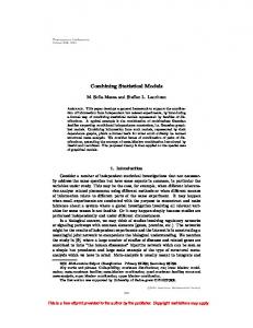
Fig. 1.11 Tube center temperature distribution through the shell for poor (a) and optimal (b) design.
Figure 1.11 illustrates the effects of the above adjustments on the key design objective – the temperature distribution along the center of each catalyst-filled tube, over the entire reactor shell. The poor case has marked temperature gradients (color contours) across the tube bundle for tubes in the same axial position. As a result of the considered adjustments to the internal geometry, the optimal case shows virtually uniform radial temperature profiles. This means that the reactants in all tubes are subject to the same or very similar external conditions at any cross section of the reactor, with no discrepancy of performance arising from the radial position of the tube within the tube bundle. It also means that the reactions occurring within the tubes – and hence conversion – are very similar for all the tubes across the bundle. Figure 1.12 shows similar information: the tube center temperature profiles for selected tubes at different radial positions. The variation across the tubes is considerable in the original, up to 40 ◦ C at certain axial positions. Figure 1.13 shows the corresponding conversions for the same tubes. In the optimal design, all tubes have a very similar conversion. Not only is overall conversion better, but the different tubes perform in a similar way, meaning that catalyst deactivation is more uniform. This results in better overall performance and longer catalyst life. 1.4.5 Discussion
The results shown here are the effects of very subtle changes, which can only be represented accurately using very high fidelity predictive modeling at all scales of the process, from catalytic reaction to shell-side fluid modeling.
1.5 Conclusions
Fig. 1.12 Tube center axial temperature profiles for selected
tubes at different radial positions for poor and optimal design.
The ability to perform this type of analysis gave the company involved a chance to perform detailed design themselves, saving millions of dollars on the engineering contract. The design exercise here resulted in a reactor capable of being brought to market as a commercial process. It is just one of many similar types of reactor modeled by various chemical companies, some far more exothermic where the effects of achieving uniform production across the tube bundle radius are far more valuable.
1.5 Conclusions
It can be seen that it is possible to tackle enormously complicated and challenging modeling tasks with today’s process modeling technology. Not only are the tools available in which to describe and solve the models, but there is a set of well-proven methodologies that provide a logical step-by-step approach to achieving high-fidelity predictive models capable of an accurate representation over a wide range of operating conditions and scales. The procedures outlined above are all readily achievable and are being applied in many different areas of the process industries.
Fig. 1.13 Axial conversion profiles for selected tubes at
different radial positions for poor and optimal design.
31
32
1 Dynamic Process Modeling: Combining Models and Experimental Data to Solve Industrial Problems
A good model can be used to explore a much wider design space than is possible via experimentation or construction of pilot plants, and in a much shorter time. This leads to “better designs faster,” with shorter times-to-market (whether the “design” is an entire new process or simply an operational improvement on an existing plant). And as has been described above, the model-based engineering approach can generate information that is simply not available via other techniques, which can be used to significantly reduce technology risk. Pilot plant testing can be reduced to the point where its sole purposes are to provide data for determining key parameters and to validate that the model is capable of predicting different states of operation accurately. What this means in broad terms for the process organization is that it is now possible to:
• • •
•
Design process, equipment and operations to an unprecedented level of accuracy. This includes the ability to apply formal optimization techniques to determine optimal solutions directly rather than rely on trial-and-error simulation. Simply by applying the procedures above to derive and apply accurate models it is possible to bring about percentage improvements in “already optimized” processes, translating to significant profits for products in competitive markets. Represent very complex processes – for example, crystallization and polymerization, or the complex physics, chemistry and electrochemistry of fuel cells – in a way that was not possible in the past. This facilitates and accelerates the design of new processes, enables reliable scale-up, and provides a quantitative basis for managing the risk inherent in any innovation. Integrate R&D experimentation and engineering, using models as a medium to capture, generate and transfer knowledge. By promoting parallel rather than sequential working, the effectiveness and speed of both activities is increased.
The ability to create models with a wide predictive capability that can be used in a number of contexts within the organization means that it is possible to recover any investment in developing models many times over. For example, models are increasingly embedded in customized interfaces and supplied to end users such as operations or purchasing personnel, who benefit from the use of model’s power in providing advice for complex decisions without having to know anything about the underlying technology. To assist this process, there is a growing body of high-fidelity models available commercially, and in equation form from university research and literature, as the fundamentals of complex processes become more and more reliably characterized. It is evident that high-fidelity predictive modeling can provide significant value, and that to realize this value requires investment in modeling (as well as a certain amount of experimentation). The key remaining challenge is to effect a change in the way that the application of modeling is perceived by process industry management and those who allocate resources, as well as in some cases the technical personnel engaged in modeling, who need to broaden their perceptions of what can be achieved.
References
References 1 Kondili, E., Pantelides, C. C., Sargent, 7 Asprey, S. P., Macchietto, S., Statistical R. W. H., A general algorithm for shorttools for optimal dynamic model building, term scheduling of batch operations – I. Computers and Chemical Engineering 24 (2000), pp. 1261–1267. MILP formulation, Computers and Chemi8 Rodriguez-Fernandez, M., Kucherenko, cal Engineering 17(2) (1993), pp. 211–227. S., Pantelides, C. C., Shah, N., Opti2 Foss, B. A., Lohmann, B., Marquardt, mal experimental design based on global W., A field study of the industrial modsensitivity analysis, in: 17th European Symeling process, Journal of Process Control 8 posium on Computer Aided Process Engineer(1998), pp. 325–338. ing – ESCAPE17, Plesu, V., Agachi, P. S. 3 Pantelides, C. C., Sargent, R. W. H., (eds.). Vassiliadis, V. S., Optimal control of mul9 Bermingham, S. K., Neumann, A. M., tistage systems described by high-index Kramer, H. J. M., Verheijen, P. J. T., van differential-algebraic equations, in: ComRosmalen, G. M., Grievink, J., A design putational Optimal Control, Bulirsch, R., procedure and predictive models for soKraft, D. (eds.), Intl. Ser. Numer. Math., lution crystallisation processes, AIChE vol. 115, Birkhäuser Publishers, Basel, Symposium Series 323 (2000), pp. 250–264, 1994, pp. 177–191. presented at the 5th International Confer4 Keskes, E., Adjiman, C. S., Galindo, A., ence on Foundations of Computer-Aided Jackson, G., Integrating advanced thermoProcess Design, Colorado, USA, 18–23 dynamics and process and solvent design July 1999. for gas, in: 16th European Symposium on Computer Aided Process Engineering and 9th 10 Shin, S. B., Han, S. P., Lee, W. J., Im, Y. H., Chae, J. H., Lee, D. I., Lee, W. H., International Symposium on Process Systems Urban, Z., Optimize terephthaldehyde Engineering, Marquardt, W., Pantelides, C. reactor operations, Hydrocarbon Process(eds.), 2006. ing (International edition) 86(4) (2007), pp. 5 Schneider, R., Sander, F., Gorak, A., 83–90. Dynamic simulation of industrial reactive 11 Baumler, C., Urban, Z., Matzopoulos, absorption processes, Chemical EngineerM., Hydrocarbon Processing (International ing and Processing 42 (2003), pp. 955–964. edition) 86(6) (2007), pp. 71–78. 6 Liberis, L., Urban, Z., Hybrid gPROMSCFD modelling of an industrial scale crys- 12 Rolandi, P. A., Romagnoli, J. A., A framework for on-line full optimizing talliser with rigorous crystal nucleation control of chemical processes, in: Proceedand growth kinetics and a full population ings of the ESCAPE15, Elsevier, 2005, pp. balance, in: Proceedings, Chemputers 1999, 1315–1320. Dusseldorf, Germany, October 21–October 22, Session 12 – Process Simulation: On the Cutting Edge.
33