Effect of Reusable Rate Variation on the Performance of Remanufacturing Systems Hasan Kivanc Aksoy and Surendra M. Gupta* Laboratory for Responsible Manufacturing 334 SN, Department of MIME Northeastern University 360 Huntington Avenue Boston, MA 02115. ABSTRACT In this paper, we investigate the variation in the reusable rate of cores (used products) on the performance of the remanufacturing system. The remanufacturing system considered here consists of three modules; viz., the disassembly and testing module for returned products, the disposition module for non-reusable returns, and the remanufacturing module. Each server in the system is subject to breakdown and has a finite buffer capacity. Repair times, breakdown times and service times follow exponential distributions. We model the remanufacturing system as an open queueing network and use the decomposition principle and expansion methodology to analyze it. Keywords: Remanufacturing, recycling, disassembly, production planning and inventory control, reusable rate, disposal, open queueing network, expansion methodology, throughput, throughput approximation, buffering.
1. INTRODUCTION The implementation of extended manufacturer responsibility together with the new more rigid environmental legislation and public awareness, has caused a growing number of manufacturers to begin recycling and remanufacturing their products (cores) after they are discarded by the consumers. In addition, the economic attractiveness of reusing products, subassemblies or parts instead of disposing them has further fueled this phenomenon. Remanufacturing is an industrial process in which worn-out products are restored to “like-new” conditions. Thus, remanufacturing provides quality standards of new products with used parts. Remanufacturing is not only a direct and preferable way to reduce the amount of waste generated, it also reduces the consumption of virgin resources. Product recovery management puts the responsibility of collection of all used and discarded products, components, materials and their reuse opportunities on the manufacturing company. The objective of product recovery management as stated by Thierry et al. is “to recover as much of the economic (and ecological) value as reasonably possible, thereby reducing the ultimate quantities of waste”15. The product recovery options include repairing, refurbishing, remanufacturing, cannibalizing and recycling. Remanufacturing operations are labor intensive that lead to significant variability in the processing times at various shop floor operations. The uncertainties surrounding the returned products further complicate the modeling and analysis of product recovery problems. As such, forecasting the quantity and the quality level of used products is difficult. There are two different types of uncertainties that affect the remanufacturing process: internal uncertainty and external uncertainty. Internal uncertainty comprises of the variations within the remanufacturing process such as the quality level of the product, the remanufacturing lead time, the yield rate of the process and the possibility of system failure. External uncertainty comprises of the variations originating from factors outside the remanufacturing process which include the timing, quantity and quality (reusable rate) of the returned products, the timing and the level of demand, and the procurement
*Correspondence: e-mail:
[email protected]; URL: http://www.coe.neu.edu/~smgupta/ Phone: (617)-373-4846; Fax: (617)-373-2921
lead times of new parts/products. The results of the aforementioned uncertainties include undersupply or obsolescence of inventory, improper remanufacturing plan and loss of competitive edge in the market. The main objective of this paper is to investigate effect of reusable rate variation on the performance of the remanufacturing planning and inventory control system. We model the remanufacturing system using an open queueing network with finite buffers and unreliable servers1. The remanufacturing system considered here consists of three modules, viz.; the testing module for returned products, the disposition module for non-reusable returns and the remanufacturing module. In order to analyze the queueing network, we use the decomposition principle and expansion methodology6, 7, 9, 10.
2. LITERATURE REVIEW This section presents a brief literature review of two closely related areas: 1) disassembly, and 2) inventory control of remanufacturing systems. The first crucial step of product recovery is disassembly. Disassembly is a methodical extraction of valuable parts/subassemblies and/or materials from post-used products through a series of operations. After disassembly, reusable parts/subassemblies are cleaned, refurbished, tested and directed to the part/subassembly inventory for remanufacturing operations. The recyclable materials can be sold to raw-material suppliers and the residuals are disposed of. The problems associated with disassembly and scheduling have been investigated by Brennan et al.2, Gupta and Taleb5, Taleb and Gupta13and Taleb et. al.14. Moyer and Gupta11 provide a comprehensive review of recycling and disassembly efforts in the electronics industry. Gungor and Gupta4 review the literature in the area of environmentally conscious manufacturing and product recovery. The problems associated with remanufacturing have been addressed by Guide and Srivastava3. Many authors have discussed the requirements to enhance recycling activity: such as ease of disassembly, modularity, material selection and compatibility, material identification and efficient cross-industrial reuse of common parts/materials. Classical models of production planning and inventory control need to be modified for remanufacturing. Heyman8 analyzed the continuous-review inventory control problem where incoming returnables are disposed of whenever the inventory reaches a predefined level. The author assumed zero repair times and did not consider procurement lead times. Muckstadt and Isaac12 developed an approximate control strategy with respect to order points and order quantities for a single product case where returned products are remanufactured. They considered fixed lead times but without disposal of returned products. Van der Laan et al.16 proposed an (s, Q) inventory control model in which used products can be remanufactured into new ones. They developed two alternative approximation methods for cost evaluation and the optimization instead of an exact analysis. Also, they showed that disposition is a necessary option because inventory levels may rise to very high values because of the variability in the return streams. Van der Laan et al.17 considered a single-product, single-echelon production and inventory system with product returns, product remanufacturing, and product disposal. For the proposed system three different procurement and inventory control strategies were considered, namely the ( s p , Q p , s d , N ) strategy, the ( s p , Q p , sd ) strategy, and the ( s p , Qp , N ) strategy. The control parameters in these strategies relate to the inventory position at which an outside procurement order is placed ( s p ) , the inventory position at which returned products are disposed of ( sd ) , the outside procurement order quantity (Qp ) , and the capacity of the remanufacturing facility (N ) . The authors derived exact expressions of the total expected costs as functions of the control parameters and compared the performance of the alternative strategies with respect to cost, under different system conditions. All the above papers assumed 100% recovery of returned products. However, one of the challenges of the remanufacturing system is to accurately estimate the percentage of reusable parts from the returned cores. Inadequate estimates can give rise to improper inventory coordination between remanufactured and new products. In this paper, we investigate the effect of reusable rate variation on the performance of remanufacturing systems.
collection of used products
testing & evaluation
disassembly
r reusable rate
remanufacturing shops
cleaning
1− r
test remanufactured parts and components
testing
sale of reproducible materials (recycling) disposition or sale as a scrap
routing to remanufacturing module
parts/ components inventory
outside procurement assembly with remanufactured, use as-is and new parts/ components
final inspection
serviceable inventory
demand
Figure 1. Remanufacturing operations and flow of jobs.
3. BACKGROUND Various remanufacturing operations and the flow of jobs are depicted in Figure 1. In the remanufacturing process, a low reusable rate of products does not, by itself, create a major problem since it is always possible to supplement the deficient amount with new parts/materials bought from outside suppliers to satisfy the demand in a given period. However, the variable reusable rate of a product complicates production and inventory planning. In Figure 1, r represents the reusable rate of the parts, which are disassembled from returned products. Generally, reusable rate r can be defined as r = 1 − sr , where sr corresponds to the scrap rate. r is a stochastic variable with mean r , standard deviation σ r , and density function f (r ) such that 0 ≤ r ≤ 1 . If we assume that the distribution of r is symmetrical, then clearly P ( X rem (t ) < X req (t )) = P ( X rem(t ) > X req (t )) = 0.5 Where X rem (t ) : denotes the output of remanufacturing operations in period t and X req (t ) : denotes the required amount of remanufactured item to satisfy the demand in period t. If Rp represents the planned reusable rate (expected recovery rate of returned products), then the following probabilities hold: Rp
Pund = P ( X rem < X req ) =
∫ F (r )dR
p
(the probability of undersupply of remanufactured products)
0
Rp
∫
Pobs = P( X rem > X req ) = 1 − F (r )dR p (the probability of obsolescence of remanufactured) 0
where F(r) is the distribution function of r. Consider a simple example. Assume that the reusable rate r for a certain type of part varies from 25% to 60% with a mean yield rate (r ) of 40%. Assume further that the extreme rates represent the 10% and 90% probability points respectively. This means that if the reusable rate were to be 25% for a certain part, we would need to procure 400 units of that part from returned products. Even at this level, the risk of undersupply would be 10% and that of oversupply (or obsolescence) would be 90%. On the other hand, if the reusable rate were 60%, we would need to procure 166.67 units of that part from returned products. In this case, the risk of undersupply would be 90% and that of obsolescence would be 10%. Finally, if mean reusable rate of 40%, were considered, we would need to procure 250 units of that part from returned products and still the
risk of undersupply and obsolescence would be 50% for each. Therefore, the costs of carrying excess inventory to provide customer satisfaction and the costs of shortage leading to lack of customer satisfaction are the main tradeoffs for handling such uncertainties in the remanufacturing environment.
4. THE MODEL AND METHODOLOGY OF INVESTIGATION A remanufacturing system can be modeled as a collection of various service areas where jobs arrive at different rates and demand services with unequal processing times. In this paper, we utilize an open queuing network (OQN) with finite buffers and unreliable servers to model the remanufacturing system. A queuing network representation of a typical remanufacturing system is depicted in Figure 2. The remanufacturing system considered here consists of three modules, viz., a testing module for returned products, a disposition module for non-reusable returns, and a remanufacturing module. The remanufacturing module consists of four different stations to accomplish the distinct operations required by the variations in the returned products. After the remanufacturing operations, items are directed to the serviceable inventory from where the demand is satisfied We assume that the demand rate, γ is greater than the product return rate, λar . Thus, outside procurement is needed to supplement any additional demand. It is assumed that when the demand is not satisfied, a lost sales cost is incurred. Similarly, when the demand is less than the inventory level, an inventory holding cost is incurred. Note that, in the queuing network, all the stations have finite buffer capacities and are prone to breakdowns. disassembly station
λar
M/M/1(BD)/K1
inspection station
remanufacturing station 1
r M/M/1(BD)/K2
M/M/1(BD)/K4
remanufacturing station 4
remanufacturing station 2
p12
M/M/1(BD)/K5
p 24
throughput of remanufacturing system
M/M/1(BD)/K7
return rate
(1-r) disassembly and testing module
p14 p13
p 23
p34
serviceable inventory
γ demand rate
M/M/1(BD)/K6 M/M/1(BD)/K3
disposition station
disposition module
remanufacturing station 3
probabilistic routings for remanufacturing module
γ − (λar × r ) outside procurement
Figure 2. Illustrative remanufacturing network with unreliable and finite buffer servers
We use the decomposition principle and the expansion methodology in order to analyze the queuing network. The decomposition principle is widely used in the analysis of a queuing network when a closed form solution for the network does not exist. The idea is to partition the network into individual nodes so that one is able to analyze and estimate the necessary parameters of each node independent of the rest of the network. When the analysis of each node is complete, the interaction of each node with the rest of the network can be reviewed. After decomposing the network, we use the expansion methodology to analyze each node individually6, 7, 9. Formulation and analysis of the expansion methodology will be discussed next. 4.1. Model Assumptions In this paper we analyze a single item, single location serviceable inventory system where returned products are remanufactured. We assume that both return and demand processes are independent. Interarrival times for returns and demand are exponentially distributed with rates λar and γ respectively. There is one server at each node and the finite buffer capacity of each server is represented by Bi . The service rate µ i for each operation is exponentially distributed and the service discipline is First Come First Serve (FCFS). The breakdown rate α i and the repair time rate β i for broken machines are also exponentially distributed. The blocking mechanism in the remanufacturing system is ‘block after service’ (BAS). When an item is ready to join a station, either the buffer at that station is not full, in which case the item joins the queue for the remanufacturing operations, or the buffer is full and the item cannot join the queue, in which case it stays where it has originated from and blocks that server. A blocked job is released to the downstream station as a space becomes available
there. The only exception is when the used products first arrive at the disassembly station from outside. In that case, if a returned product finds the buffer of the station full, it cannot enter the remanufacturing system and is considered lost to the system. However in this situation, because of potential recoverability of the returned product a penalty cost is applied. A remanufactured unit is instantly directed to the serviceable inventory from where the demand is satisfied. Any deficiency is fulfilled with outside procurement of new products. The transfer times of items between buffers and stations are assumed to be negligible. When a failure of a station occurs during the processing of a part, the part stays there while the station is being repaired. After the repair of the station, the part is reprocessed from the beginning. Note that, assumptions in our model differ from the typical production line models reported in the literature. The first difference is that our model considers the buffer capacities to be finite rather than the typical assumption of being infinite. Most importantly, a common assumption in the production line models is that the first station of the production line is never starved and the last station of the line is never blocked. However, in our remanufacturing line model, since the return products arrive at the remanufacturing facility according to a Poisson arrival stream, a situation could occur when there are no products at the first station (disassembly station), i.e. the first station could starve. In addition, since there is a limited buffer capacity at the last station (serviceable inventory) and the demand follows a Poisson stream, the buffer at the last station could be full blocking the upstream stations. 4.2 Analysis of the Remanufacturing System We analyze the remanufacturing system by monitoring the total cost and the mean processing time of the system. The analysis here is based on the steady-state behavior of the given remanufacturing system with the following parameter set: λ ar , return rate of used products; γ , demand rate; µ i , service rate at the node i; α i , breakdown rate of node i; β i , repair rate of the node i and Bi , buffer capacity of node i. To capture the gross effect of the varied system parameters we define the total cost function based on the remanufacturing network in Figure 2. 4
TC = c p E ( RP) + c d E ( D ) + c t E (T ) + c dis E ( Dis) +
∑c
ri
E ( Ri ) + c m E (OP ) + c hs E ( I ) + cl E ( Ls ) + c rej E ( Rej )
i =1
where: cd : c dis : c hs : cl : cm : cp : ct : c ri : cr 4 : c rej : E(RP): E(D): E(T): E(Dis): E(Ri ): E(OP): E(I): E(Ls): E(Rej): PT: r: TC:
disposition cost/item. disassembly cost/item. inventory holding cost/item. lost sales cost/item. outside procurement/manufacturing cost/item. purchase cost of cores/item. testing cost/item. remanufacturing operations cost/item (i=1, 2, 3). final inspection cost/item. penalty cost of rejected returned products from the system/item. expected number of returned products. expected number of disposed products. expected number of tested products. expected number of disassembled products. expected number of remanufactured products by remanufacturing node i (i=1, 2, 3). expected number of products procured from outside suppliers. expected number of on hand inventory. expected number of lost sales. expected number of rejected items from the system. mean processing time. reusable rate of returned products. average total cost of the remanufacturing system.
To obtain the approximate throughput rates of each server and the entire remanufacturing network, we utilize the expansion methodology. In this section we briefly discuss the fundamentals of the expansion methodology. Details of the method and necessary derivations for unreliable production lines can be obtained from Gupta and Kavusturucu6, 7 and Kavusturucu and Gupta9. The expansion methodology is an efficient tool for the analysis of nodes with finite buffers. In order to analyze the remanufacturing system, which is presented in Figure 2, we first decompose the network and examine each server separately. After isolating each node we expand the network by adding a node in front of the each server. These extra nodes are modeled as infinite buffer nodes with zero processing times. They act as “holding nodes” for jobs, which cannot enter the destination node because the buffer is full. The blocked jobs stay there until a space becomes available at the full buffer. Next, the parameters that define the expanded network, such as the actual arrival rate to the system, the probability of a job being blocked by the full buffer, etc. are calculated. Finally, using the newly calculated parameters, the throughput of the entire network can be calculated10.
5. NUMERICAL EXPERIMENTATION In order to analyze the remanufacturing system given in Figure 2, we investigate six scenarios. Unless otherwise mentioned, Tables 1 and 2 provide the values of the system parameters in all scenarios.
Table 1. Routing probabilities pij in the remanufacturing shop.
i/j 1 2 3 4
1 -
2 0.5 -
3 0.4 0.8 -
Table 2. System parameters and cost variables for base-case scenario.
4 0.1 0.2 1 -
γ = 1.0 cd = 5 cdis = 6 cl = 5 cm = 25
cp = 4 ct = 1 cri = 5 (i=1, 2, 3). chs = 1 crej = 5
The six scenarios considered are as follows: Scenario 1: This is the base case scenario where, in addition to Tables 1 and 2 parameter values, ( µ i , α i , β i , Bi ) = (1.5, 0.2, 2. 3) for all i = 1,…, 7. Scenario 2: This is similar to Scenario 1 except for the modification in certain cost parameters. The cost parameters that are modified and their new values are: cd = 10, ct = 2, cri = 3, 3, 5. Scenario 3: This is similar to Scenario 1 except for the parameter value ( Bi ) = (9) for all i = 1,…, 7. Scenario 4: This is similar to Scenario 1 except for the parameter values ( µ i , α i , β i ) = (2, 0.1, 1) for all i = 1,…, 7. Scenario 5: This is similar to Scenario 1 except for the parameter values ( α i , β i , Bi ) = (0.2, 2, 3 – 0.4, 3, 9 – 0.2, 2, 3 – 0.4, 3, 9 – 0.2, 2, 3 – 0.1, 1, 9 – 0.2, 2, 9), for i = 1,…, 7 respectively. Scenario 6: This is similar to Scenario 1 except for the parameter values ( µ i , α i , β i ) = (1.2, 0.1, 1) for all i = 1,…, 7, and B i = (3 – 9 – 9 – 3 –3 – 3 – 9), for i = 1,…, 7 respectively.
9 7
T.C. for r=0.8
Core return rate
Figure 7. Scenario 5.
P.T. for r=0.6 P.T. for r=0.8 T.C. for r=0.4
Total cost
T.C. for r=0.8
5
15 0.1
1
17 0.9
T.C. for r=0.6
6 0.8
19
0.7
7
10
Total cost
P.T. for r=0.4 P.T. for r=0.6 P.T. for r=0.8 T.C. for r=0.4 T.C. for r=0.6 T.C. for r=0.8
1
0.9
0.8
5 0.7
T.C. for r=0.8
15
0.6
T.C. for r=0.6
0.5
T.C. for r=0.4
20
0.4
P.T. for r=0.8
25
0.3
P.T. for r=0.6
30 28 26 24 22 20 18 16 14 12 10
30
0.2
Total cost
P.T. for r=0.4
Mean process time
35
0.1
1
0.9
0.8
0.7
0.6
T.C. for r=0.8
Figure 6. Scenario 4.
30 28 26 24 22 20 18 16 14 12 10 0.5
T.C. for r=0.6
Core return rate
25 23 21 19 17 15 13 11 9 7 5 0.4
T.C. for r=0.4
P.T. for r=0.4
Total cost
21
Figure 5. Scenario 3.
0.3
P.T. for r=0.8
1
8
Core return rate
0.2
0.9
23
0.6
T.C. for r=0.8
25
9
1
0.9
0.8
0.7
0.6
0.5
0.4
0.3
0.2
0.1
5
T.C. for r=0.6
27
0.5
10
T.C. for r=0.4
29
10
0.4
15
P.T. for r=0.8
31
11
0.3
20
P.T. for r=0.6
12
0.2
25
P.T. for r=0.4
Mean process time
30
Total cost
30 28 26 24 22 20 18 16 14 12 10
35
0.1
P.T. for r=0.6
Figure 4. Scenario 2.
40 Mean process time
P.T. for r=0.4
Core return rate
Figure 3. Scenario 1.
Mean process time
0.8
0.1
Core return rate
0.7
5
1
0.9
0.8
0.7
0.6
0.5
0.4
0.3
0.2
0.1
5
T.C. for r=0.6
11
0.6
7
T.C. for r=0.4
13
0.5
9
P.T. for r=0.8
15
0.4
11
P.T. for r=0.6
0.3
13
P.T. for r=0.4
17
0.2
15
35 33 31 29 27 25 23 21 19 17 15
19 Mean process time
Mean process time
17
Total cost
30 28 26 24 22 20 18 16 14 12 10
19
Core return rate
Figure 8. Scenario 6.
The results of the six scenarios are given in Figures 3 - 8. From these results,, the following conclusions can be drawn: • In Scenario 1 (Figure 3), the remanufacturing and disposal costs are lower than the outside procurement cost. In this situation, remanufacturing of products is worthwhile to consider. From figure 3 it is clear that the higher the reusability rate (r), the lower the total cost for all core return rates. As the core return rate increases, the total cost decreases. Similarly, lower expected reusability rate (r = 0.4) results in a lower mean process time and vice versa. • When the core return rates are low, the total cost is relatively insensitive to the reusability rate. However, as the core return rate becomes higher the reusability rate has a significant effect on the total cost. The higher the reusability rate, the lower the total cost. • Mean process time (average remanufacturing time) is sensitive to the buffer size, breakdown rate, repair rate and service rate of the stations in the remanufacturing system. Variability in the buffer sizes in the network causes a significant
•
variation in the mean process time (Figure 8). Similar behavior is also observed when the buffer levels are high in the entire network (Figure 5). Service rate can also effect the mean process time as is evident from Figures 6 and 7.
REFERENCES 1. 2. 3. 4. 5. 6. 7. 8. 9. 10. 11. 12. 13. 14. 15. 16. 17.
Aksoy, H. K. and Gupta, S. M., “An open queueing network model for remanufacturing systems”, Proceedings of the 25th. Conference on Computers and Industrial Engineering, pp. 62-65, New Orleans, LA, March 29-31, 1999. Brennan., L., Gupta, S. M. and Taleb, K. N., “Operations planning issues in an assembly/disassembly environment”, International Journal of Operations and Production Planning, 14(9), 57-67, 1994. Guide, Jr., V. D. R. and Srivastava, R., “Buffering from material recovery uncertainty in a recoverable manufacturing environment”, Journal of the Operational Research Society, 48, 519-529, 1997. Gungor, A. and Gupta, S. M., “Issues in environmentally conscious manufacturing and product recovery: a survey”, Computers and Industrial Engineering, 36, 811-853, 1999. Gupta, S. M. and Taleb, K. N., “Scheduling disassembly”, International Journal of Production Research, 32, 18571866, 1994. Gupta, S. M. and Kavusturucu, A., “Modeling of finite buffer cellular manufacturing systems with unreliable machines”, International Journal of Industrial Engineering, 5(4), 265-277, 1998. Gupta, S. M. and Kavusturucu, A, “Production systems with interruptions, arbitrary topology and finite buffers”, Annals of Operations Research, 93, 145-176, 2000. Heyman, D. P., “Optimal disposal policies for a single item inventory system with returns”, Naval Research Logistics Quarterly, 24, 385-405, 1977. Kavusturucu, A. and Gupta, S. M., “Analysis of Manufacturing flow lines with unreliable machines”, International Journal of Computer Integrated Manufacturing, 12(6), 510-524, 1999. Kerbache, L. and Smith, J. M., “Asymptotic behavior of the expansion method for open finite queueing networks”, Computers and Operations Research, 15(2), 157-169, 1988. Moyer, L. K. and Gupta, S. M., “Environmental concerns and Recycling/Disassembly Efforts in the electronic industry”, Journal of Electronics Manufacturing, 7(1), 1-22, 1997. Muckstadt, J. and Isaac, M. H., “An analysis of single item inventory systems with returns”, Naval Research Logistics Quarterly, 28, 237-254, 1981. Taleb, K. N. and Gupta, S. M., “Disassembly of multiple product structures”, Computers and Industrial Engineering, 32, 949-961, 1997. Taleb, K N., Gupta, S. M. and Brennan, L., “Disassembly of complex product structures with parts and materials commonality”, Production Planning and Control, 8, 255-269, 1997. Thierry, M., Salomon, M., van Nunen, J., and van Wassenhove, L., “ Strategic issues in product recovery management”, California Management Review 37(2), 114-135, 1995. van der Laan, E., Dekker, R., Salomon, M. and Ridder, A., “An (s,Q) inventory model with remanufacturing and disposal”, International Journal of Production Economics, 46(47), 339-350, 1996. van der Laan, E., Dekker, R. and Salomon, M., “Product remanufacturing and disposal: a numerical comparison of alternative control strategies” International Journal of Production Economics, 45, 489-498 1996.