TEDI: Efficient Shortest Path Query Answering on Graphs Fang Wei Computer Science Department University of Freiburg Freiburg, Germany
[email protected]
ABSTRACT
1. INTRODUCTION
Efficient shortest path query answering in large graphs is enjoying a growing number of applications, such as ranked keyword search in databases, social networks, ontology reasoning and bioinformatics. A shortest path query on a graph finds the shortest path for the given source and target vertices in the graph. Current techniques for efficient evaluation of such queries are based on the pre-computation of compressed Breadth First Search trees of the graph. However, they suffer from drawbacks of scalability. To address these problems, we propose TEDI, an indexing and query processing scheme for the shortest path query answering. TEDI is based on the tree decomposition methodology. The graph is first decomposed into a tree in which the node (a.k.a. bag) contains more than one vertex from the graph. The shortest paths are stored in such bags and these local paths together with the tree are the components of the index of the graph. Based on this index, a bottom-up operation can be executed to find the shortest path for any given source and target vertices. Our experimental results show that TEDI offers ordersof-magnitude performance improvement over existing approaches on the index construction time, the index size and the query answering.
Querying and manipulating large scale graph-like data have attracted much attention in the database community, due to the wide application areas of graph data, such as ranked keyword search, XML databases, bioinformatics, social network, and ontologies. The shortest path query answering in a graph is among the fundamental operations on the graph data. In a ranked keyword search scenario over structured data, people usually give scores by measuring the link distance between two connected elements. If more than one path exists, it is desirable to retrieve the shortest distance between them, because shorter distance normally means higher rank of the connected elements [19, 20, 12]. In a social network application such like Facebook 1 , registered users can be considered as vertices and edges represent the friend relationship between them. Normally two users are connected through different paths with various lengths. The problem of retrieving the shortest path among the users efficiently is of great importance. Let G = (V, E) be an undirected graph where n = |V |. Given u, v ∈ V , the shortest path problem finds a shortest path from u to v with respect to the length of paths from u to v. One obvious solution for the shortest path problem is to execute the Breadth First Search (BFS) on the graph. The time complexity of the BFS method is O(n). If the graph is of large size, the efficiency of query answering is expected to be improved. The query answering can be performed in constant time, if the BFS tree for each vertex of the graph is pre-computed. However, the space overhead is n2 . This is obviously not affordable if n is of large value. Therefore, appropriate indexing and query scheme for answering shortest path queries must find the best trade-off between these two extreme methods. Xiao et al.[23] proposed the concept of compact BFS-trees where the BFS-trees are compressed by exploiting the symmetry property of the graphs. It is shown that the space cost for the compact BFS trees is reduced in comparison to the normal BFS trees. Moreover, shortest path query answering is more efficient than the classic BFS-based algorithm. However, this approach suffers from scalability. Although the index size of the compact BFS-trees can be reduced by 40% or more (depending on the symmetric property of the graph), the space requirement is still prohibitively high. For instance, for a graph with 20 K vertices, the compact BFStree has the size of 744 MB, and the index construction takes
Categories and Subject Descriptors H.3.3 [Information Search and Retrieval]: Search process; H.3.1 [Content Analysis and Indexing]: Indexing methods
General Terms Algorithms, Design
Keywords graphs, indexing, shortest path, tree decomposition
Permission to make digital or hard copies of all or part of this work for personal or classroom use is granted without fee provided that copies are not made or distributed for profit or commercial advantage and that copies bear this notice and the full citation on the first page. To copy otherwise, to republish, to post on servers or to redistribute to lists, requires prior specific permission and/or a fee. SIGMOD’10, June 6–11, 2010, Indianapolis, Indiana, USA. Copyright 2010 ACM 978-1-4503-0032-2/10/06 ...$10.00.
1
http://www.facebook.com
more than 30 minutes. Therefore, this approach can not be applied for graphs with larger size which contain hundreds of thousands of vertices.
1.1 Our Contributions To overcome these difficulties, we propose TEDI (TreE Decomposition based Indexing), an indexing and query processing scheme for the shortest path query answering. Briefly stated, we first decompose the graph G into a tree in which each node contains a set of vertices in G. These tree nodes are called bags. Different from other partitioning based methods, there are overlapping among the bags, i.e., for any vertex v in G, there can be more than one bag in the tree which contains v. However, it is required that all these related bags constitute a connected subtree (see Definition 1 for the formal definition). Based on the decomposed tree, we can execute the shortest path search in a bottom-up manner and the query time is decided by the height and the bag cardinality of the tree, instead of the size of the graph. If both of these two parameters are small enough, the query time can be substantially improved. Of course, in order to compute the shortest paths along the tree, we have to pre-compute the local shortest paths among the vertices in every bag of the tree. This constitutes the major part of the index structure of the TEDI scheme. Our main contributions are the following: • Solid theoretical background. TEDI is based on the well-known concept of the tree decomposition, which is proved being of great importance in computational complexity theory. The abundant theoretical results provide a solid background for designing and correctness proofs of the TEDI algorithms. • Linear time tree decomposition algorithm. In spite of the theoretical importance of the tree decomposition concept, many results are practically useless due to the fact that finding a tree decomposition with optimal treewidth is an NP-hard problem, w.r.t. the size of the graph. To overcome this difficulty, we propose in TEDI the simple heuristics to achieve a linear time tree decomposition algorithm. To the best of our knowledge, TEDI is the first scheme that applies the tree decomposition heuristics dealing with graphs of large size, and based on that, enables efficient query answering algorithms to be developed. • Flexibility of balancing the time and space efficiency. From the proposed tree decomposition algorithm, we discover an important correlation between the query time and the index size. If less space for the index is available, we can reduce the index size by increasing some parameter k during the tree decomposition process, while the price to pay is longer query time. On the other hand, if the space is less critical, and the query time is more important, we can decrease k to achieve higher efficiency of the query answering. This flexibility offered by TEDI enables the users to choose the best time/space trade-off according to the system requirements.
performance improvement over existing algorithms. Moreover, we conduct the experiments over large graphs such as DBLP and road networks. The encouraging results show that TEDI scales well on large datasets. The rest of the paper is organized as follows: in Section 2 we introduce the formal definitions of the tree decomposition and prove the theoretical results regarding to the shortest path query answering. Section 3 contains the detailed algorithms and the complexity analysis. In Section 4 we present the experimental results. We survey related works in Section 5 and conclude in Section 6.
2. GRAPH INDEXING WITH TREE DECOMPOSITION 2.1 Tree Decomposition An undirected graph is defined as G = (V, E), where V = {0, 1, . . . , n − 1} is the vertex set and E ⊆ V × V is the edge set. Let n = |V | be the number of vertices and m = |E| be the number of edges. In this paper, we consider only undirected graphs, where ∀u, v ∈ V : (u, v) ∈ E ⇔ (v, u) ∈ E holds. Moreover, we assume that the edges are not labeled. In the rest of the paper, we will use the term graph to denote undirected graph. Definition 1 (Tree Decomposition). A tree decomposition of G = (V, E), denoted as TG , is a pair ({Xi | i ∈ I}, T ), where {Xi | i ∈ I} is a collection of subsets of V and T = (I, F ) is a tree such that: S 1. i∈I Xi = V . 2. for every (u, v) ∈ E, there is i ∈ I, s.t. u, v ∈ Xi . 3. for all v ∈ V , the set {i | v ∈ Xi } induces a subtree of T. A tree decomposition consists of a set of tree nodes, where each node contains a set of vertices in V . We call the sets Xi bags. It is required that every vertex in V should occur in at least one bag (condition 1), and for every edge in E, both vertices of the edge should occur together in at least one bag (condition 2). The third condition is usually referred to as the connectedness condition, which requires that given a vertex v in the graph, all the bags which contain v should be connected. Note that from now on, the node in the graph G is referred to as vertex, and the node in the tree decomposition is referred to as tree node or simply node. For each tree node i, there is a bag Xi consisting of vertices. To simplify the presentation, we will sometimes use the term node and its corresponding bag interchangeably. Given a tree decomposition TG , we denote its root as R. Given any graph G, there may exist many tree decompositions which fulfill all the conditions in Definition 1. However, we are interested in those tree decompositions with smaller bag sizes. We call the cardinality of a bag the width of the bag. Definition 2 be a graph.
(Width, Treewidth). Let G = (V, E)
• The width of a tree decomposition ({Xi | i ∈ I}, T ) is Finally we conduct experiments on real and synthetic datasets, defined as max{|Xi | | i ∈ I} 2 . and compare the results with the compact BFS-tree ap2 proach. The experimental results confirm our theoretical The original definition of the width is max{|Xi | | i ∈ I}−1, analysis by demonstrating that TEDI offers orders-of-magnitude due to technical reasons.
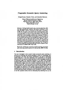
• The treewidth of G is the minimal width of all tree decompositions of G. It is denoted as tw(G) or simply tw. Example 1. Consider the graph illustrated in Figure 1(a). One of the tree decompositions is shown in Figure 1(b). The width of this tree decomposition is 3. It is not hard to check that this tree decomposition is optimal, thus the treewidth of the graph is 3.
({4, 0}, {3, 0}), ({4, 3}, {1, 3}), ({4, 0}, {5, 0}), . . .. Note that it is possible that the same pair of vertices occurs in more than one bag. For instance, the edge (4, 3) occurs in both bags X0 and X1 . Thus there are two inner edges: ({4, 1}, {3, 1}) and ({4, 0}, {3, 0}). In order to traverse from one bag to another in the tree decomposition, we need to define the second kind of edge, the inter edge. Note that two neighboring bags in the tree are in fact connected by the common vertices they share, according to the connectedness condition in Definition 1. Definition 4 (Inter edge). Let G = (V, E) be a graph and TG = ({Xi | i ∈ I}, T ) a tree decomposition of G. Let v ∈ Xi and v ∈ Xj , where either (i, j) ∈ F or (j, i) ∈ F holds. We call the edge from vertex {v, i} to {v, j} the inter edge and denote it as ({v, i}, {v, j}).
(a)
(b)
Figure 1: The graph G (a) and one tree decomposition TG (b) with tw = 3 Induced subtree. Let G = (V, E) be a graph and TG = ({Xi | i ∈ I}, T ) a tree decomposition of G. Due to the third condition in Definition 1, for any vertex v in V there exists an induced subtree of TG in which every bag contains v. We call it the induced subtree of v and denote it as Tv . Furthermore, we denote the root of Tv as rv and its corresponding bag as Xrv . For instance, X0 , X1 and X2 constitute the bags of the induced subtree of vertex 3 in Figure 1(b), because vertex 3 occurs precisely in these three bags. Since X0 is the root of the induced subtree, we have r3 = 0.
2.2 Tree Path Let G = (V, E) be a graph, and u, v ∈ V . v is reachable from vertex u, denoted as u → v, if there is a path starting from u and ending at v with the form {u, v1 , . . . , vn , v}, where (u, v1 ), (vi , vi+1 )(1≤i≤n−1) , (vn , v) ∈ E. The shortest distance from vertex u to vertex v is denoted as sdist(u, v). Note that in this paper, we consider only simple paths. Obviously, for undirected graphs, u → v ⇔ v → u. Let us consider the graph vertices in the tree nodes. Since a vertex in G may occur in more than one bag of TG , it is identified with {v, i}, where v is the vertex and i the node in the tree, meaning that vertex v is located in the bag Xi . We denote it as tree vertex. Now we define the so-called internal edge in the tree decomposition. Recall that the second condition in Definition 1 requires that for every edge (u, v) ∈ E, both u and v should occur in some bag of TG . We call these edges inner edges in the tree decomposition. Definition 3 and TG = ({Xi | i inner edges of TG follows: {({u, i}, {v, i}) |
(Inner edge). Let G = (V, E) be a graph ∈ I}, T ) a tree decomposition of G. The are the pairs of tree vertices defined as (u, v) ∈ E, u, v ∈ Xi (i ∈ I)}
Intuitively, the set of inner edges consists of precisely those edges in E, with the extra information of the bags in which the edges are located. For instance, the inner edges of the tree decomposition of the graph in Example 1 are: ({0, 2}, {5, 2}), ({1, 3}, {2, 3}), ({2, 1}, {3, 1}), ({3, 2}, {0, 2}), ({4, 1}, {3, 1}),
For instance, in Example 1, ({5, 0}, {5, 2}) is an inter edge, as well as ({5, 2}, {5, 0}), because vertex 5 occurs in bags X0 and X2 , where 0 is the parent node of 2. Now we are ready to define the tree path on the tree decomposition with inner and inter edges. Definition 5 (Tree path). Let G = (V, E) be a graph and TG = ({Xi | i ∈ I}, T ) a tree decomposition of G. Let u, v ∈ V . Let further {u, i} and {v, j} be tree vertices in TG . A tree path from {u, i} to {v, j} is a sequence of tree vertices connected with either inter or inner edges. Lemma 1. Let G = (V, E) be a graph and TG = ({Xi | i ∈ I}, T ) a tree decomposition of G. Let u, v ∈ V . Let further {u, i} and {v, j} be tree vertices in TG . There is a path from u to v in G if and only if there is a tree path from {u, i} to {v, j}. Proof. The ”if” direction is trivial: given a tree path from {u, i} to {v, j}, we only need to consider the inner edges. Since for each inner edge {u, i}, {v, i}, there is an edge (u, v) ∈ E, the path from u to v can be easily constructed. Now we prove the ”only if” direction: assume that there is a path from u to v in G. We prove it by induction on the length of the path. • Basis: if u reaches v with a path of length 1, that is, (u, v) ∈ E. Then there exists a node k in the tree decomposition, s.t. u ∈ Xk and v ∈ Xk . We start from {u, i}, traverse along the induced subtree of u, till we reach {u, k}. Since the induced subtree is connected, the path from {u, i} to {u, k} can be constructed with inter edges. Then we reach from {u, k} to {v, k} with an inner edge. Now we traverse from {v, k} to {v, j} along the induced subtree of v, which can again be constructed with inter edges. The tree path from {u, i} to {v, j} is thus completed. • Induction: assume that the lemma holds with paths whose length is less than or equal to n − 1, we prove that it holds for paths with length of n. Assume that there is a path from u to v with length n, where u reaches w with length n − 1 and (w, v) ∈ E. From induction hypothesis, we know that there is a tree path form {u, i} to {w, l} in the tree decomposition, where l is a node in the induced subtree of w. Since (w, v) ∈ E, there is a node n such that w ∈ Xn and v ∈ Xn . Thus {w, n} can be reached from {w, l} with inter edges.
Then {w, n} can reach {v, n} with an inner edge. Finally {v, n} can reach {v, j} with a sequence of inter edges. This completes the proof.
Example 2. Consider the graph in Figure 1(a). Vertex 4 reaches vertex 0 with the path (4, 1, 2, 3, 0). In the tree decomposition in Figure 1(b), there is a tree path from {4, 1} to {0, 2} as follows: ({4, 1}, {4, 3}, {1, 3}, {2, 3}, {2, 1}, {3, 1}, {3, 0}, {3, 2}, {0, 2}).
2.3 Shortest Path Query Answering on Tree Decomposition With the definition of the tree path, we are able to map every path from u to v in the graph G into a tree path in the corresponding tree decomposition TG . Since all the paths can be traced in the tree decomposition, after inspecting all the corresponding tree nodes, we are able to compute the shortest path from u to v. Our goal is now to restrict the attention of the tree nodes to those that every tree path would pass through. There is a well-known property of trees that for any two nodes i and j in a tree, there exists a unique simple path, denoted as SPi,j , such that every path from i to j contains all the nodes in SPi,j . In the following we show that this property can also be applied to tree paths. Given a tree path P in the tree decomposition, we say P visits a node i , if there is a tree vertex {v, i} in P .
The following question thus arises: Can we compute the shortest path from u to the vertices (respectively from the vertices to v) in the simple path more efficiently? The answer is yes. Intuitively, we can compute the shortest distance from u to the vertices occur in the simple path bag after bag, in a bottom-up manner. Let us assume that the current bag be Xc and its parent bag be Xp . Assume further that for all the vertices t ∈ Xc , we have obtained sdist(u, t). Now we start processing Xp . For any vertex s ∈ Xp \ Xc , the following property holds: sdist(u, s) = {min(sdist(u, t) + sdist(t, s)) | t ∈ Xc ∩ Xp } This is because every path from u to s has to pass through one vertex in Xc ∩ Xp (formal proof given in Theorem 2). Therefore, the shortest path must be among them. Clearly, in order to enable the bottom-up operation, we need to store the shortest distances for each bag in the tree decomposition. That is, in every bag X, for every pair of vertices x, y ∈ X, we pre-compute sdist(x, y) and store them locally. In addition to the local shortest distance, we need to store the vertices in sdist(x, y), denoted as path(x, y), to trace back the vertices along the shortest path later on.
Lemma 2. Let {u, i} and {v, j} be two tree vertices, and SPi,j be the simple path between tree nodes i and j. Let P be a tree path from {u, i} to {v, j}. Then P visits every node in SPi,j . Example 3. The tree path from {4, 1} to {0, 2} shown in Example 2 visits the nodes in a sequence of (1, 3, 1, 0, 2). It contains not only all the nodes in the simple path, but also node 3, which is not in the simple path. Theorem 1. Let G = (V, E) be a graph and TG = ({Xi | i ∈ I}, T ) a tree decomposition of G. Let u, v ∈ V , and ru (resp. rv ) be the root node of the induced subtree of u (resp. v). Then for every node w in SPru ,rv , there is one vertex t ∈ Xw , such that sdist(u, v) = sdist(u, t) + sdist(t, v). Proof. Let p be the shortest path from u to v in G that generates sdist(u, v). From Lemma 1, we know that there is a corresponding tree path P of p from {u, ru } to {v, rv } in TG . According to Lemma 2, P visits all the nodes in SPru ,rv . Then for every node n in SPru ,rv , there is a vertex {t, n} in P . Therefore, t is in p. Then we have sdist(u, v) = sdist(u, t) + sdist(t, v). Theorem 1 shows that for every path from u to v in G, although the tree path from {u, ru } to {v, rv } may possibly visit any node in the tree, we only need to concentrate on those vertices which occur in the simple path SPru ,rv . More precisely, we can simply take any node w from SPru ,rv , and for each t ∈ Xw , compute sdist(u, t) and sdist(t, v) respectively. Then, the minimal value of sdist(u, t) + sdist(t, v) is the shortest distance from u to v. However, this is obviously not a solution, since we have to compute the shortest path for 2c times, where c is the cardinality of the bag Xw .
Figure 2: Bottom-up processing on the simple tree path Given the tree decomposition of G and the local shortest distance, as well as u and v, the shortest path query answering is sketched in Theorem 2. See Figure 2 for a graphical illustration. Theorem 2. Let G = (V, E) be a graph and u, v ∈ V . Let tw be the treewidth of G and TG = ({Xi | i ∈ I}, T ) be the corresponding tree decomposition. The shortest distance from u to v can be computed in O(tw2 h), where h is the height of TG . Proof. We show that the bottom-up operation can be executed on TG , so that the shortest distance (as well as the corresponding shortest path) from u to v can be computed. Let us make the following assumptions of TG : Tu (resp. Tv ) is the induced subtree of u (resp. v) where ru (resp. rv ) is the root. a is the youngest common ancestor of ru and rv , Assume further that the shortest distance (sdist) and shortest path (path) for the pairs of vertices in every bag in TG are pre-computed. We explain the process only for the side of u, the bottom-up process from the v side is identical. The process starts with the node ru . From the information of shortest distance in the tree node Xru , we can simply obtain sdist(u, t) for each t ∈ Xru .
Next, we consider ru as the child node and process its parent node, with the available sdist information. This process is executed till a is reached. We show that at each step of the processing, the shortest distance from u to all the vertices in the current bag can be computed in w2 time, where w is the width of the current bag. Assume p is the current node, c its child node, and we have obtained sdist(u, t) for each t ∈ Xc . Now we have to compute the shortest distance from u to every vertex in Xp . Let z be a vertex in Xp . We want to compute sdist(u, z). We consider the following two cases: 1. z ∈ Xp and z ∈ Xc . Since at the child node sdist(u, z) is already obtained, the value sdist(u, z) remains unchanged. 2. z ∈ Xp and z ∈ / Xc . This is a more complex case. We show that there is a vertex t, where t ∈ Xp and t ∈ Xc , such that sdist(u, z) = sdist(u, t) + sdist(t, z). In other words, the shortest path from u to z has to pass through some vertex t which occurs in both Xc and Xp . Since z does not occur in Xc , according to the connectedness condition, z does not occur in any bag in the subtree rooted with c. Thus the induced subtrees of u and z do not share any common node in TG . Since u → z, there is a tree path from {u, ru } to {z, rz }, and c, p ∈ SPru ,rz . The tree path from {u, ru } to {z, rz } must contain an inter edge of the form ({t, c}, {t, p}), where t ∈ Xp , Xc , because this is the only possible edge to traverse from c to p. Therefore, the shortest path from u to z must pass through one vertex t ∈ Xp , Xc . Given the shortest distance from u to every vertex in Xc , we compute the shortest distance from u to the vertices in Xp as follows: First for each vertex t ∈ Xc ∩ Xp , set sdist(u, t) the same value as in Xc . Then for each vertex t ∈ Xp \ Xc , set sdist(u, t) = min(sdist(u, s)+sdist(s, t)) where s ∈ Xc ∩Xp . Clearly the time consumption is in the worst case O(w2 ) where w is the width of Xp . To sum up, at each step, the time cost of updating the shortest distance is O(tw2 ), where tw is the treewidth of G. and there are maximally 2h steps where h is the height of the tree decomposition. Hence the overall time cost is O(tw2 h).
3.
ALGORITHMS AND COMPLEXITY RESULTS
In this section, we present the detailed algorithms for both the index construction and the shortest path query answering. In Section 3.1 we begin with the introduction of algorithmic issues on the tree decomposition from a complexity theory perspective, and then justify our choice of an efficient but suboptimal decomposing algorithm. In Section 3.2 we first analyze the shortest path query answering algorithm proposed in Theorem 2 from the previous section. Then, we point out that the time and space improvement can be made to achieve more efficiency of our algorithm.
3.1 Index Construction via Tree Decomposition The index construction algorithm consists of three steps (see Algorithm 1). Step 1 and 2 constitute the major part of the index construction task: decomposing the graph G.
Algorithm 1 index construction(G) Input: G = (V, E) Output: TG and local shortest paths. 1: graph reduction(k, G); {output the vertex stack S and reduced graph G′ } 2: tree decomposition(S, G, G′ ); {output the tree decomposition TG } 3: local shortest paths(G, TG ); {compute local shortest paths in TG }
Since its introduction by Robertson and Seymour [18], the concepts of tree decomposition has been proved to be of great importance in computational complexity theory. The interested readers may refer to an introductory survey by Bodlaender [4]. The theoretical significance of the tree decomposition based approach lies in the fact that many intractable problems can be solved in polynomial time (or even in linear time) for graphs with treewidth bounded by a constant. Problems which can be dealt with in this way include many well known NP-complete problems, such as the Independent Set, the Hamiltonian Circuits, etc. Recent applications of tree decomposition based approaches can be found in Constraint Satisfaction [15] and database design [10]. However, the practical usefulness of tree decomposition based approaches has been limited due to the following two problems: (1) Computing the treewidth of a graph is hard. In the last section, we have always assumed that a tree decomposition is given. In fact, to obtain a tree decomposition with the minimal width (treewidth) is a optimization problem. Determining whether the treewidth of a given graph is at most a given integer w is NP-complete [2]. Although for a fixed w, linear time algorithms exist to solve the decision problem ”treewidth ≤ w”, there is a huge hidden constant factor, which prevents it from being useful in practice. There exist many heuristics and approximation algorithms for determining the treewidth, unfortunately few of them can deal with graphs containing more than 1000 vertices [17]. (2) The second problem lies in the fact that even if the treewidth can be determined, good performance for solving intractable problems by using the tree decomposition based approaches can only be achieved if the underlying structure has bounded treewidth (i.e. less than 10). Because the time complexity of most of the algorithms is exponential to the treewidth. As far as the efficiency is concerned, we can only search for an approximate solution, which yields a suboptimal treewidth. On the other hand, we can tolerate a treewidth which is not bounded. As we have seen from Theorem 2, the time complexity is in the worst case quadratic of the treewidth (width). We will show later in this section that our query answering algorithm does not depend on the treewidth, but with some parameter which can be enforced to be bounded, due to the nice property of our dedicated decomposing algorithm. Inspired by the so-called pre-processing methods from Bodlaender et al. [5], we apply the reduction rules on the graph by reducing stepwise a graph to another one with fewer vertices, due to the following simple fact. Definition 6 (Simplicial). A vertex v is simplicial in a graph G if the neighbors of v form a clique in G. Proposition 1. If v is a simplicial vertex in a graph G,
computing the treewidth of G is equivalent to computing the treewidth of G − v. Proof. Let TG−v be the tree decomposition of G − v. Let further {v1 , . . . , vl } be the neighbors of v. We construct a bag Xc = {v, v1 , . . . , vl }. Since {v1 , . . . , vl } form a clique, there exists a bag in TG−v consisting of all the vertices in {v1 , . . . , vl }. We denote it as Xp . We can then construct TG by adding Xc as a child of Xp . It is easy to verify that all the conditions of the tree decomposition are fulfilled. Thus this new tree is also a tree decomposition. Now consider the treewidth of TG . Xc has the size of l +1. It is easy to show that the size of Xp is equal to or greater than l + 1, thus by adding the new bag Xc the treewidth remains to be the same. Figure 3 shows some special cases. If a vertex v has degree of one (Figure 3(a)), then we can remove v without increasing the treewidth. Figure 3(b), 3(c) illustrate the cases of degree 2 and 3 respectively.
Algorithm 2 graph reduction(k, G) Input: graph G, k is the upper bound for the reduction. Output: stack S and the reduced graph G′ 1: initialize stack S; 2: for i = 1 to k do 3: remove upto(i); 4: end for 5: return S, G; 6: procedure remove upto(l) 7: while TRUE do 8: if there exists a vertex v with degree less than l then 9: {v1 , . . . , vl } = neighbors of v; 10: build a clique for {v1 , . . . , vl } in G; 11: push v, v1 , . . . , vl into S; 12: delete v and all its edges from G; 13: else 14: break; 15: end if 16: end while
bound k for the reduction, so that the program stops after the degree-k reduction. Note that as the degree increases, the effectiveness of the reduction will decrease, because in the worst case, we need to add l(l − 1)/2 edges in order to remove l edges. (a)
(b)
(c)
Figure 3: A graph containing a vertex v with degree 1 (a), 2 (b) and 3 (c) The main idea of our decomposition algorithm is to reduce the graph by removing the vertices one by one from the graph, and at the same time push the removed vertices into a stack, so that later on the tree can be constructed with the information from the stack. Each time a vertex v with a specific degree is identified. We first check whether all its neighbors form a clique, if not, we add the missing edges to construct a clique. Then v together with its neighbors are pushed into the stack, which is followed by the deletion of v and the corresponding edges in the graph. See Algorithm 2. The program begins with removing isolated vertices and vertices with degree 1. Then, the reduction process proceeds by increasing the degree of the vertex. We denote such procedure of removing all the vertices with degree l as degree-l reduction. Example 4. Consider the graph in Example 1. Figure 4 illustrates the reduction process. The process starts with a degree-2 reduction by removing vertex 0 and its edges, after adding the edge between 3 and 5. Vertex 0 and its neighbors are then pushed in the stack. Then vertex 1 is removed, following the same principle as of 0. After vertex 2 is removed, a single triangle is then left. Algorithm 2 will terminate if one of the following conditions is fulfilled. (1) The graph is reduced to an empty set. For instance, if the graph contains only simple cycles, it will be reduced to an empty set after degree-2 reductions. This is usually the case for extremely sparse graphs. (2) For graphs which are not sparse, one has to define a upper
Figure 4: The reduction process on the graph of Example 1 After the reduction process, the tree decomposition can be constructed as follows: (1) At first we collect all the vertices which were not removed by the reduction process and assign this set as the bag of the tree root R. The size of R depends on the structure of the graph (i.e. how many vertices are left after the reduction). For graphs which are not sparse, the bag size of the root is the greatest among all bags in the tree decomposition. (2) The rest of the tree is generated from the information stored in stack S. Let Xc be the set of vertices {v, v1 , . . . , vl } which is popped up from the top of S. Here v is the removed vertex and {v1 , . . . , vl } are the neighbors of v which form a clique. After the parent bag Xp which contains {v1 , . . . , vl } is located in the tree, Xc is added as a child bag of Xp . This process proceeds until S is empty. Algorithm 3 illustrates the process. The last step of the index construction is to compute and store the shortest distances and paths for every pair of vertices in the bags of the tree decomposition (see Algorithm 4). We apply the standard BFS algorithms. Due to the property of the tree decomposition, there exist redundancies. For instance, both node 1 and 3 in Figure 1(b) contain the vertex pair (2, 4). Therefore, the same shortest distance
Algorithm 3 tree decomposition(S, G, G′ ) Input: S is the stack storing the removed vertices and their neighbors, G is the graph, G′ is the reduced graph of G. Output: return tree decomposition TG 1: construct the root of TG containing all the vertices of G′ ; 2: while S is not empty do 3: pop up a bag Xc = {v, v1 , . . . , vl } from S; 4: find the bag Xp containing {v1 , . . . , vl }; 5: add Xc into T as the child node of Xp ; 6: end while Algorithm 4 local shortest paths(G, TG ) Input: G, TG Output: local shortest paths in TG 1: for all bag X in the tree decomposition do 2: for every vertex pair x, y ∈ X do 3: compute sdist(x, y) and path(x, y) 4: end for 5: end for
is stored in two bags. This redundancy can be avoided by storing the shortest distances in a hash table.
3.2 Shortest Path Query Answering Recall from Theorem 2 that the time complexity of the bottom-up query answering is O(tw2 h). This upper bound is optimal, only if the following two conditions are fulfilled: (1) the treewidth of the underlying graph is bounded (that is, tw2 ≪ n), and (2) there is an efficient tree decomposition algorithm for it. The first condition has to be fulfilled, since otherwise the linear time BFS algorithm would be more efficient. Unfortunately, as we have seen in Section 3.1, given an arbitrary graph, neither of them can be guaranteed. Therefore, we have to inspect the tree decomposition heuristics applied in Section 3.1 for improvements.
3.2.1 From Treewidth to |R| and k According to Algorithm 2, a graph G can be decomposed by the degree-l reductions by increasing l from 1 to k. As soon as the degree-k reduction is done, all the vertices which are not yet removed are the elements in R of the tree decomposition. Usually if the graph is not extremely sparse, the relationship k ≪ |R| holds. In fact, we could even enforce such a relationship by setting k to be small enough in the tree decomposition algorithm. Hence, the resulting tree decomposition has the following properties: (1) the root is of big size (|R|), and (2) the rest of the bags have smaller size (the upper bound is k). If we inspect the bottom-up query processing more carefully, we could observe that the quadratic time computation over the root can be always be avoided. To see this, let us consider the vertices u and v and the youngest common ancestor of ru and rv is the root R. Assume that X1 (resp. X2 ) is the child node of R which locates in the simple path from ru (resp. rv ) to R. Consider now that for all x ∈ X1 , sdist(u, x) (resp. all y ∈ X2 , sdist(y, v)) have been computed. Clearly, any path from u to v has to pass through a vertex in X1 and X2 respectively. Therefore, at the root node R, the interface from X1 to R has to be X1 ∩ R, and accordingly, the interface from X2 to R has to be X2 ∩ R.
Now, we only need to execute a nested loop on X1 ∩ R and X2 ∩ R, to decide the final shortest path. Since both |X1 | and |X2 | have the upper bound of k, the overall time consumption is of O(k2 h), thus independent of |R|. The algorithm for the shortest path query answering is presented in Algorithm 5. Comparing with the bottom-up query processing shown in Theorem 2, Algorithm 5 is customized with respect to our dedicated tree decomposition algorithm, in the sense that the query time complexity is adapted to be related to k, instead of the treewidth. Given the graph G, its tree decomposition TG and the pre-computed local shortest paths in the bags on TG , as well as the vertices u, v, we first locate the root of the induced subtree of u (v), denoted as ru (rv ). The algorithm considers special cases, according to the relationship between ru and rv . (1) if ru and rv are located in one bag, then the shortest path can be immediately returned (line 4). (2) Otherwise, we have to locate the youngest common ancestor of ru and rv , denoted as root. Here a special case is either ru or rv is root. If this occurs, the bottom-up operation should be only executed from one side. Note that we stop the processing at the child node of the root node. At each step of the bottomup processing, we update the shortest distance value, as well as the parent value, for the later backtrace for the shortest path(line 11 and 19). As soon as both the child nodes X1 and X2 are reached, we obtain the common values with the root node by executing the set intersection operation with it (line 25). At last, a nested loop over the bag X1 and X2 is executed, to stitch the threads from both sides. Finally, the shortest path can be traced back using the p set we have stored during the bottom-up processing.
3.3 Complexity Index construction time. For the index construction, we have to (1) generate the tree decomposition, and (2) at each tree node, generate the required shortest paths. For (1), both of the reduction step and the tree construction procedure take time O(n). For (2), we deploy the classic BFS algorithm, which costs in worst case O(n). In fact, we need to run for each vertex in G exactly one BFS procedure. Therefore, the overall index construction time is O(n2 ). Index size. In each bag X, for each pair of vertices u, v in X, we need to store the vertices along the shortest path between u and v. Thus the index size is l|X|2 , where l is the average length of all the local shortest paths. Since the relationship k ≪ |R| holds, the root size (|R|) is dominant among all the bags. Therefore, the index size is l|R|2 . The index size consists of the tree structure, constructed by using the tree decomposition algorithm. However, this space overhead is linear to n, thus can be ignored. Query. The bottom-up query processing for shortest path computation takes time O(k2 h), where k is the number of the reductions and h is the height of the tree decomposition.
3.3.1 The Trade-off between Time and Space The number of the reductions for the tree decomposition algorithm, k, and the root size |R|, represent the trade-off between the time and space consumptions of the TEDI approach. As analyzed above, the time complexity for the query answering depends on k, whereas the index size is decided by |R|. Clearly, regarding to the tree decomposition algorithm, |R| is a monotonically decreasing function of k. Usually, |R| decreases drastically as k is small, e.g. from 1 to
5. Then, the decreasing of |R| follows diverse trends, which is decided by the characteristics of the underlying graphs. One obvious instance is that for extremely sparse graphs, |R| can be decreased rapidly into zero after 3 or 4 steps of reductions. For instance, the graph “Eva” in Figure 5 belongs to this category. However, this correlation can not be solely reflected by the density of the underlying graph. An exact investigation of such a relationship is left as the future work. Figure 5 depicts the k-|R| relationship for the real datasets we have tested. In this illustration, the Y-axis depicts the value of |R|/n in percentage, namely the proportion of the root size with respect to the graph size. Note that due to the wide range of the value on Y-axis, we plot the vertical axis logarithmically. More details of the dataset are given in Section 4. 100
Root Size/Graph Size(%)
Algorithm 5 reach dist(TG , u, v) Input: TG is the tree decomposition of G and u, v vertices in G. In every bag X of TG , and any pair of x, y ∈ X, sdist(x, y) stores the shortest distance, and path(x, y) stores the vertices along the path. Output: the shortest path from u to v. 1: ru = root of induced subtree of u; 2: rv = root of induced subtree of v; 3: if (ru == rv ) then 4: return path(u, v); 5: end if 6: root = youngest common ancestor of ru and rv ; 7: if (ru == root) then 8: switch u and v; switch ru and rv ; 9: end if 10: for all x ∈ Xru do 11: label x with du (x) = sdist(u, x); p(x) = u; 12: end for 13: X1 = Xru ; 14: while X1 .parent 6= root do 15: Xp = X1 .parent 16: for all t ∈ Xp \ X1 do 17: for all s ∈ Xp ∩ X1 do 18: if du (t) > du (s) + sdist(s, t) then 19: du (t) = du (s) + sdist(s, t); p(t) = s; 20: end if 21: end for 22: end for 23: X1 = Xp ; 24: end while 25: X1 = X1 ∩ root; 26: if rv is the ancestor of ru then 27: X2 = {v}; dv (v) = 0; 28: else 29: for all x ∈ Xrv do 30: label x with dv (x) = sdist(v, x); p(x) = v; 31: end for 32: X2 = Xrv ; 33: while X2 .parent 6= root do 34: Xp = X2 .parent 35: for all t ∈ Xp \ X2 do 36: for all s ∈ Xp ∩ X2 do 37: if dv (t) > dv (s) + sdist(s, t) then 38: dv (t) = dv (s) + sdist(s, t); p(t) = s; 39: end if 40: end for 41: end for 42: X2 = Xp ; 43: end while 44: X2 = X2 ∩ root; 45: end if 46: mdist = {min(du (x)+dv (y)+sdist(x, y)) | (x ∈ X1 , y ∈ X2 }; 47: let x ∈ X1 , y ∈ X2 be the vertices along the shortest path; 48: while x! = u do 49: output path(x, p(x)); x = p(x); 50: end while 51: output path(x, y); 52: while y! = v do 53: output path(y, p(y)); y = p(y); 54: end while
Pfei Geom Epa Dutch Erdos PPI Eva Cal Yea Homo Inter
10
0
5
10
15 k
20
25
30
Figure 5: k and |R| relationships for real data
4. EXPERIMENTAL RESULTS In this section we evaluate the TEDI approach on real, synthetic, and large datasets respectively, for the shortest path query answering. All tests are run on an Intel(R) Core 2 Duo 2.4 GHz CPU, and 2 GB of main memory. All algorithms are implemented in C++ with the Standard Template Library (STL). We are interested in the following parameters: • Index size, • Index construction time, and • Query time. The index size consists of two parts: (1) the size of the tree decomposition. This includes the tree structure and the vertices stored in the bags of the tree decomposition. (2) the local shortest paths stored in the hash table, which is dominant comparing to part (1). The index construction time consists of two parts as well: (1) time cost for the tree decomposition. (2) the time for the local shortest path generation. Here part (2) is dominant. Besides the standard measurements, we are also interested in the structure of the tree decomposition, which may influence the performance of the algorithm. These are: • the number of tree nodes (#TreeN), • the number of all the vertices stored in the bags (#SumV),
in Table 3. Surprisingly, the speedup for all the datasets, except for one graph, is higher than that of SYMM. In summary, TEDI algorithm is superior to SYMM in all aspects.
• the height of the tree (h), • the number of vertex reductions (k), and • the root size of the tree. (|R|). In our experiments, we compare our approach with the compact BFS trees proposed by Xiao et al. [23], which we denote as SYMM. To the best of our knowledge, SYMM is the state-of-the-art implementation for efficient shortest path query answering with pre-computed index structures.
4.1 Real Datasets We test a variety of real graph data including biological networks (PPI, Yea and Homo), social networks (Pfei, Geom, Erdos, Dutch, and Eva), information networks (Cal and Epa) and technological networks (Inter). All the graph data are provided by the authors of [23]. Some statistics of the graphs w.r.t. the tree decomposition algorithm are shown in Table 1. Note that we have chosen the optimal k, in order to achieve the best query time performance. Graph Pfei Gemo Epa Dutsch Eva Cal Erdos PPI Yeast Homo Inter
n 1738 3621 4253 3621 4475 5925 6927 1458 2284 7020 22442
#TreeN 1680 3000 3637 3442 4457 5095 6690 1359 1770 5778 21757
#SumV 3916 9985 11137 8700 9303 18591 18979 3638 6708 24359 67519
h 16 10 7 9 9 14 9 11 6 10 10
k 6 5 7 5 2 10 7 7 9 15 13
|R| 60 623 618 258 75 832 405 101 516 1244 687
Table 1: Statistics of real graphs and the properties of the index We measure the time and space cost of the index construction on the real datasets, and compare our results with SYMM [23]. See Table 2 for details. The index size generated with TEDI has been dramatically reduced comparing with SYMM. In fact, most of the index sizes of TEDI are two orders of magnitude smaller than those generated with SYMM. For the index construction time, improvement can be shown similarly. The index construction time of TEDI on every graph is at least one order of magnitude faster than that with SYMM. The measurement on the index construction time and the index size confirms the complexity analysis in Section 3.3.1. The index construction time is only dependent on the graph size, whereas the index size is decided by the root size |R|. For instance, the graph size of Homo is 3 times small than Inter, while the root size is two times greater than Inter. This is exactly reflected by the index size and index construction time in Table 2 respectively. We execute the query answering algorithm given in Algorithm 5. For each dataset we randomly generate 10000 pairs of vertices and query the shortest paths between each pair of vertices. To make a fair comparison, we have implemented the naive BFS algorithm. This way, we could compare the speedup of our method w.r.t BFS algorithm to the speedup of the SYMM algorithm w.r.t. BFS. The results are shown
Graph Pfei Gemo Epa Dutsch Eva Cal Erdos PPI Yeast Homo Inter
TEDI (ms) 0.003420 0.002933 0.002096 0.002655 0.002299 0.003325 0.002037 0.002629 0.002463 0.007666 0.004178
TEDI BFS 0.052 0.123 0.105 0.097 0.089 0.187 0.146 0.050 0.071 0.226 0.693
SYMM [23] Speedup 13.04 41.10 39.62 28.21 20.20 59.31 57.72 13.30 25.63 N.a. N.a.
Speedup 15.2 42.4 50.0 37.3 38.7 56.7 71.9 19.2 28.4 29.7 169.0
Table 3: Comparison between TEDI and SYMM on query time over real dataset.
4.2 Synthetic Data We have generated synthetic graphs according to the BA model [3], a widely used model to simulate real graphs. To make a fair comparison, we set k = 1.1, so that the average degree of the graph generated is 2k, which is identical to the synthetic datasets in [23]. We vary the graph size from 1000 to 10000 vertices by the step of 1000. Graph 1k 2k 3k 4k 5k 6k 7k 8k 9k 10k
n 1000 2000 3000 4000 5000 6000 7000 8000 9000 10000
#TreeN 808 1730 2641 3559 4460 5355 6292 7201 8089 8983
#SumV 2131 4786 7362 10131 12758 15371 18626 20790 23497 26224
h 9 11 10 10 10 10 12 11 12 11
k 3 5 6 7 8 9 9 9 9 9
|R| 194 272 361 443 542 612 710 801 913 1019
Table 4: Statistics of the synthetic graphs and the properties of the index Some statistics of those graphs w.r.t. the tree decomposition algorithm are shown in Table 4. Again, we have chosen the optimal k, in order to achieve the best query time performance. The measurement of the index construction time and index size is similar to those of real dataset. The index size and the index construction time are shown in Table 5. Figure 6(a) and 6(b) illustrate the comparison of index construction time and the index size on the synthetic datasets with SYMM. Note that due to the wide range of time and space cost, we plot the vertical axis logarithmically. The results in Figure 6(a) and 6(b) show clearly that on both the index size and the index construction time, TEDI outperforms the approach SYMM with the improvement of more than an order of magnitude. Since SYMM does not present the query time for the synthetic data, we can not make a comparison on that. Instead,
Graph Pfei Gemo Epa Dutsch Eva Cal Erdos PPI Yeast Homo Inter
Index Size (MB) tree TEDI SYMM [23] 0.008 0.033 7.9243 0.020 1.830 44.9907 0.022 1.652 28.1992 0.016 0.420 20.8559 0.018 0.044 5.5447 0.038 3.078 92.026 0.018 0.534 32.2695 0.008 0.060 5.954 0.014 1.094 19.4457 0.048 6.928 21.574 0.136 1.796 744.07478
paths 0.025 1.81 1.63 0.404 0.026 3.04 0.516 0.052 1.08 6.88 1.66
ttree 0.003 0.068 0.056 0.011 0.006 0.145 0.038 0.004 0.019 0.198 0.796
Index Time (s) tpaths TEDI SYMM [23] 0.099 0.102 2.688 0.878 0.946 14.859 0.97 1.026 37.14 0.311 0.322 13.687 0.239 0.245 289.532 2.535 2.680 34.094 0.849 0.887 90.453 0.130 0.134 1.547 0.566 0.585 7.578 7.745 7.943 53.985 15.858 16.654 1709.64
Table 2: Comparison between TEDI and SYMM on index construction of real dataset.
Graph 1k 2k 3k 4k 5k 6k 7k 8k 9k 10k
Comparison of Index Construction Time (s) 100 TEDI SYMM
10
Index Size (MB) paths tree TEDI 0.27 0.004 0.274 0.61 0.010 0.620 1.16 0.014 1.174 1.76 0.020 1.780 2.68 0.025 2.705 4.0 0.030 4.030 4.6 0.036 4.636 6.2 0.042 6.242 8.2 0.047 8.247 10.2 0.052 10.052
Index Time ttree tpaths 0.003 0.088 0.010 0.217 0.024 0.385 0.038 0.625 0.040 0.953 0.081 1.340 0.092 1.942 0.091 2.400 0.124 3.128 0.167 4.274
(s) TEDI 0.091 0.227 0.409 0.663 0.993 1.456 2.134 2.491 3.252 4.441
Table 5: Index Construction of synthetic dataset 1
0.1 1k
2k
3k
4k
5k
6k
7k
8k
9k
10k
(a) Comparison of Index Size (MB) 100
we report the query time on synthetic graphs with TEDI and compare the results with the BFS algorithms. The results is given in Table 6. Interestingly, the speedup to the naive BFS method increases, as the size of the graph grows. This observation will be confirmed in the next section, namely on very large datasets, the speedup of the query time to BFS can be increased substantially.
TEDI SYMM
10
1
0.1 1k
2k
3k
4k
5k
6k
7k
8k
9k
10k
(b) Figure 6: Comparison of index construction time and size on synthetic data
Graph 1k 2k 3k 4k 5k 6k 7k 8k 9k 10k
Query Time TEDI (ms) BFS Speedup 0.001545 0.027 17.5 0.002073 0.050 25.0 0.002645 0.078 29.5 0.003286 0.104 31.6 0.003674 0.145 39.5 0.004155 0.168 40.4 0.004450 0.193 43.4 0.004754 0.226 47.5 0.005135 0.257 50.0 0.005722 0.299 52.3
Table 6: TEDI query time on synthetic datasets
4.3 Scalability over Large Datasets To test the scalability of our approach, we conduct the experiments on much larger datasets. We have chosen two datasets. The first one is DBLP dataset. We first gener-
ate an undirected graph from the DBLP N-triple dump 3 . The dataset contains all the inproceeding records and all proceedings records, with all their persons, publishers, series and relations between persons and inproceedings. To highlight the purpose of shortest path query answering, we removed elements in each paper that are not interesting to keyword search, such as url, ee, etc. Finally, we get a graph containing 593K vertices. The second large dataset is the road network of the San Francisco Bay area 4 denoted as BAY. The graph contains 321K vertices. 100
Graph DBLP BAY
Index Size (MB) paths tree TEDI 117.2 2.6 119.8 24.7 2.6 27.3
Root Size/Graph Size(%)
(s) TEDI 2226.4 3041.9
Table 8: Index construction of large dataset.
reason for this is that the average shortest path length of BAY graph is much longer than that of DBLP. Therefore, the time cost of the BFS algorithm for BAY is greater than DBLP.
DBLP BAY
Graph DBLP BAY
10
Index Time ttree tpaths 102.4 2124.0 182.2 2859.7
TEDI (ms) 0.055 0.258
Query Time BFS (ms) 32.47 20.54
Speedup 590.0 80.0
Table 9: Comparison of TEDI query time on large datasets to BFS
1
0.1 0
10
20
30
40
50
60
70
5. RELATED WORK
The classic shortest path algorithm deploys Breadth First Search, which can be implemented with a queue [16]. In Figure 7: k and |R| relationships for large data recent years, many efficient algorithms with preprocessing have been proposed for finding the shortest paths. The graphs under consideration have some special constraints Figure 7 illustrates the relationship of k and |R| w.r.t. such as edge weights. See [8, 11]. A survey paper on varithe reduction step of the tree decomposition process. Table ous versions of algorithms are presented in [9]. All of these 7 shows some characteristics of the graphs. The curves in methods are based on heuristics designed specifically on the Figure 7 exposes distinct features of the k − |R| relationship underlying datasets (like GIS data). It is unknown, whether on DBLP and BAY. For DBLP, the root size |R| can hardly the algorithms can be extended to dealing the other graph be reduced after 4000 (approximately 0.67% of the graph datasets. Moreover, one assumption common to all those size). On the other hand, the root size of BAY remains dealgorithms is that the whole graph can be stored in main creasing continuously. The results of the tree decomposition memory. reflect these differences. The decomposed tree of BAY has Another related graph query problem – which is more ina much smaller root size than that of DBLP (245 vs. 3821). tensively studied in the database community – is the reachHowever, the height of BAY is correspondingly greater than ability query answering. Many approaches have been proDBLP (30 vs. 351). This implies that the BAY dataset posed to first pre-compute the transitive closure, so that the requires less space for index structure, but the query time reachability queries can be more efficiently answered comis longer. For DBLP, the query time is much shorter beparing to BFS or DFS. The 2-HOP approach [7] proposes cause of the smaller height of the tree, but the price to pay selecting a small amount of vertices that can be stored as is greater index size. All of these observations are reflected landmark to facilitate the query answering. However, the in the Table 8 and 9. time cost for generating such an optimized vertex set is too high to be practical (O(n3 )). Some approximation algoGraph n #TreeN #SumV h k |R| rithms to 2-HOP are proposed [19]. Another category of DBLP 592 983 589 164 1 309 710 30 100 3821 reachability query answering algorithms is so-called interBAY 321 272 321 028 1 298 993 351 80 245 val labeling approach [1, 22, 6, 21, 14]. These methods first extract some tree from the graph, then store the transitive Table 7: Statistics of large graphs and the properties closure of the rest of the vertices. Good performance has of the index been obtained for sparse graphs. Recently, Jin et al. have proposed the 3-HOP algorithm for reachability query anThe experimental result on large graphs demonstrate clearly swering on dense graphs [13]. None of these methods can that the TEDI approach scales well on large dataset. Morebe extended to cope with the shortest path query answerover, the query time speedup is more substantial, in coming. Given u, v in a graph, reachability queries require only parison to the relatively smaller graphs. a boolean answer (yes or no). Therefore, the transitive cloAs far as the index time is concerned, the experimental sure stored in the index can be drastically compressed, as 2 results are against the complexity analysis of O(n ). The long as the boolean query can be correctly answered. On the 3 http://www4.wiwiss.fu-berlin.de/bizer/d2rq/benchmarks other hand, shortest path queries require that the paths to 4 http://www.dis.uniroma1.it/∼challenge9/download.shtml be returned. Therefore, the compression methods with the k
information loss can not be adapted for answering shortest path queries.
6.
CONCLUSIONS AND FUTURE WORK
In this paper, we introduced an indexing and query answering scheme based on the tree decomposition concept for the shortest path query answering. The careful theoretical analysis has shown that our approach is intuitive and efficient. Through extensive experiments over various datasets, we demonstrate that TEDI achieves the improvement of performance by more than an order of magnitude in all aspects including query time, index construction time and index size. Moreover, the algorithm scales well over large datasets. In the future we plan to investigate the following problems: (1) Development more heuristics for the tree decomposition algorithms. (2) The integration of A* heuristics for a more efficient query answering. (3) Maintenance of the index structure. Furthermore, we will consider on-disk algorithms for both index construction and query answering.
7.
REFERENCES
[1] R. Agrawal, A. Borgida, and H. V. Jagadish. Efficient management of transitive relationships in large data and knowledge bases. In SIGMOD, 1989. [2] S. Arnborg, D. G. Corneil, and A. Proskurowski. Complexity of finding embeddings in a k-tree. SIAM J. Algebraic Discrete Methods, 8(2):277–284, 1987. [3] A. L. Barabasi and R. Albert. Emergence of scaling in random networks. Science, 286(5439), October 1999. [4] H. L. Bodlaender. A tourist guide through treewidth. Acta Cybernetica, 11:1–23, 1993. [5] H. L. Bodlaender, A. M. C. A. Koster, and F. van den Eijkhof. Pre-processing rules for triangulation of probabilistic networks. Computational Intelligence, 21(3):286–305, 2005. [6] L. Chen, A. Gupta, and M. E. Kurul. Stack-based algorithms for pattern matching on dags. In VLDB, 2005. [7] E. Cohen, E. Halperin, H. Kaplan, and U. Zwick. Reachability and distance queries via 2-hop labels. SIAM J. Comput., 32(5):1338–1355, 2003. [8] A. Goldberg and C. Harrelson. Computing the shortest path: A* search meets graph theory. In SODA. SIAM, 2005.
[9] A. V. Goldberg. Point-to-point shortest path algorithms with preprocessing. In SOFSEM (1), 2007. [10] G. Gottlob, R. Pichler, and F. Wei. Tractable database design through bounded treewidth. In PODS, pages 124–133, 2006. [11] R. Gutman. Reach-based routing: A new approach to shortest path algorithms optimized for road networks. In ALENEX. SIAM, 2004. [12] H. He, H. Wang, J. Yang, and P. S. Yu. Blinks: ranked keyword searches on graphs. In SIGMOD. ACM, 2007. [13] R. Jin, Y. Xiang, N. Ruan, and D. Fuhry. 3-hop: a high-compression indexing scheme for reachability query. In SIGMOD. ACM, 2009. [14] R. Jin, Y. Xiang, N. Ruan, and H. Wang. Efficiently answering reachability queries on very large directed graphs. In SIGMOD, 2008. [15] K. Kask, R. Dechter, J. Larrosa, and A. Dechter. Unifying tree decompositions for reasoning in graphical models. Artif. Intell., 166(1-2):165–193, 2005. [16] D. E. Knuth. Art of Computer Programming, Volume 1: Fundamental Algorithms (3rd Edition). 1997. [17] A. Koster, H. L. Bodlaender, and S. P. M. V. Hoesel. Treewidth: Computational experiments. In Electronic Notes in Discrete Mathematics, pages 54–57. Elsevier Science Publishers, 2001. [18] P. D. Robertson, Neil; Seymour. Graph minors iii: Planar tree-width. Journal of Combinatorial Theory, Series B 36:49–64, 1984. [19] R. Schenkel, A. Theobald, and G. Weikum. Efficient creation and incremental maintenance of the hopi index for complex xml document collections. In ICDE, pages 360–371, 2005. [20] T. Tran, H. Wang, S. Rudolph, and P. Cimiano. Top-k exploration of query candidates for efficient keyword search on graph-shaped (rdf) data. In ICDE. IEEE, 2009. [21] S. Trissl and U. Leser. Fast and practical indexing and querying of very large graphs. In SIGMOD, 2007. [22] H. Wang, H. He, J. Yang, P. S. Yu, and J. X. Yu. Dual labeling: Answering graph reachability queries in constant time. In ICDE, 2006. [23] Y. Xiao, W. Wu, J. Pei, W. Wang, and Z. He. Efficiently indexing shortest paths by exploiting symmetry in graphs. In EDBT, 2009.