particles that fly over the fitness landscape in search of an optimal solution. The particles are controlled by forces that encourage each particle to fly back both ...
Exploring Extended Particle Swarms: A Genetic Programming Approach Riccardo Poli
Cecilia Di Chio
William B. Langdon
Department of Computer Science University of Essex, UK {rpoli,
cdichi, wlangdon}@essex.ac.uk
ABSTRACT
bees and ants are the best-known examples. Swarm intelligence offers a way to design intelligent systems (swarm systems) in which functions such as autonomy, emergence and distribution have replaced some less “natural” ones, e.g. control, programming and centralisation [5]. The class of swarm systems is a rich source of novel computational methods that can solve difficult problems efficiently and reliably. One of the best-developed techniques of this type is Particle Swarm Optimisation (PSO) [9]. PSOs use a population of candidate solutions (interacting particles) that fly over the fitness landscape and, controlled by forces that encourage each particle to fly back towards both the best point sampled by it and the swarm best, search for an optimal solution to a given problem. The forces act to over come the particle’s momentum, which tries to keep the particle moving in the same direction at the same speed. A variety of improvements to the basic form of PSO have been proposed and tested in the literature. As a result, it is very hard for a practitioner to decide what is the best PSO to use to solve a particular problem. This research is part of a project that aims to systematically categorise PSOs and explore extensions of particle swarms by including strategies from biology, by extending the physics of the particles and by providing a solid theoretical and mathematical basis for the understanding and problem-specific design of new particle swarm algorithms. We take a purely computational approach, first pioneered in [17], where the force generating equations which control the particles in a PSO are automatically evolved through the use of genetic programming (GP). Interesting PSOs were evolved in this way in [17]. However, the exploration was limited by the use of the same ingredients present in the original PSO model by Kennedy and Eberhart, namely: the position and velocity of a particle, the position of the particle best and the position of the swarm best. The aim of the research presented here is to independently verify the findings of [17] and to extend the search by considering additional meaningful ingredients for the PSO force-generating equations, such as global measures of dispersion and position of the swarm. These are believed to be very important so as to provide a way of adapting the nature of the forces used depending on the current situation of the swarm as a whole. Our results indicate that indeed GP can explore this extended space of possible PSOs, finding update rules that outperform human-generated as well as some previously evolved ones. Naturally, not all PSOs evolved can have be seen as having a connection with natural swarms, but this is not un-
Particle Swarm Optimisation (PSO) uses a population of particles that fly over the fitness landscape in search of an optimal solution. The particles are controlled by forces that encourage each particle to fly back both towards the best point sampled by it and towards the swarm’s best point, while its momentum tries to keep it moving in its current direction. Previous research started exploring the possibility of evolving the force generating equations which control the particles through the use of genetic programming (GP). We independently verify the findings of the previous research and then extend it by considering additional meaningful ingredients for the PSO force-generating equations, such as global measures of dispersion and position of the swarm. We show that, on a range of problems, GP can automatically generate new PSO algorithms that outperform standard human-generated as well as some previously evolved ones.
Categories and Subject Descriptors I.2.8 [Artificial Intelligence]: Problem Solving, Control Methods, and Search
General Terms Performance
Keywords Particle Swarm Optimisation, Swarm Intelligence, Genetic Programming
1.
INTRODUCTION
Researchers use the expression swarm intelligence to refer to the emergent collective intelligence of groups of simple agents, of which colonies of social insects such as termites,
Permission to make digital or hard copies of all or part of this work for personal or classroom use is granted without fee provided that copies are not made or distributed for profit or commercial advantage and that copies bear this notice and the full citation on the first page. To copy otherwise, to republish, to post on servers or to redistribute to lists, requires prior specific permission and/or a fee. GECCO’05, June 25–29, 2005, Washington, DC, USA. Copyright 2005 ACM 1-59593-010-8/05/0006 ...$5.00.
169
• vi is the it h component of the velocity vector v = (v1 , · · · , vN ).
usual in computational intelligence. For example, also in the field of neural networks researchers started from biologically inspired neurons. However, later research focused on nonbiologically plausible models, such as the back-propagation rule, because of their interesting and useful properties. We expect something like this might happen in the field of PSOs. This paper is part of an effort to extend PSO models beyond real biology and physics and push the limits of swarm intelligence into the exploration of swarms as they could be. Section 2 provides a brief review of the work on particle swarms to date. Since we build on [17], Section 3 describes in detail [17]’s use of GP to automatically generate and evolve PSOs tailored to particular tasks. In Section 4 we describe and motivate our variations on [17]’s basic approach. Section 5 describes our results and compares them to the performance of previously designed or evolved PSOs. Finally, Section 6 briefly restates our findings and lists potential future directions for research.
2.
In particular, in the simplest version of PSO, each particle is moved by two elastic forces, one attracting it with random magnitude to the fittest location so far encountered by the particle, and one attracting it with random magnitude to the best location encountered by any member of the swarm. More precisely, ai = φ1 R1 (xsi − xi ) + φ2 R2 (xpi − xi ) where • R1 and R2 are two independent random variables uniformly distributed in [0, 1], and • φ1 and φ2 are two learning rates which control the relative proportion of cognition and social interaction in the swarm. The velocity of a particle v and its position x are updated every time step using the equations:
PARTICLE SWARM OPTIMISATION
PSO is a method for optimisation of continuous nonlinear functions, discovered through the simulation of a simplified social model (particle swarm) [10]. PSO has its roots in two main component methodologies:
vi (t) = vi (t − 1) + ai
xi (t) = xi (t − 1) + vi (t)
As this system can lead the particles to become unstable, with their speed increasing without control, the standard technique to avoid this happening is to bound velocities so that vi ∈ [−Vmax , +Vmax ]. Early variations in PSO techniques involved the addition of analogues of physical characteristics to the members of the swarm, such as the “inertia weight” ω [18], where the velocity update equation is modified as follows:
• artificial life (ALife), in particular flocking, schooling and swarming theory, and • evolutionary computation (EC). In PSOs, which are inspired by flocks of birds and shoals of fish, a number of simple entities (the particles) are placed in the parameter space of some problem and each evaluates the fitness at its current location. Unique to the concept of PSO is “flying” over potential solutions through the hyperspace, accelerating towards better ones. Each particle determines its movement through the space by combining some aspect of the history of its own fitness values with those of one or more members of the swarm, and then moves through the parameter space with a velocity determined by the locations and processed fitness values of those other members, possibly together with some random perturbations. The next iteration takes place after all particles have been moved. Eventually the swarm as a whole is likely to move close to the best location. More formally, in the case of an N dimensional problem, each particle’s position, velocity and acceleration, can each be represented as a vector with N components (one for each dimension). In the original version of PSO, the equation controlling the particles is of the form ai = F (xi , xsi , xpi , vi )
(2)
vi (t) = ωvi (t − 1) + ai
(3)
As in vector notation the velocity change can be written as ∆v = a − (1 − ω)v, the constant 1 − ω effectively acts as a friction coefficient. Following Kennedy’s graphical examinations of the trajectories of individual particles and their responses to variations in key parameters [8] the first real attempt at providing a theoretical understanding of PSO was the “surfing the waves” model presented by Ozcan [15]. Clerc developed a comprehensive 5-dimensional mathematical analysis of the basic PSO system [7]. A particularly important contribution of that work was the use and analysis of a modified update rule: vi (t) = κ(vi (t − 1) + ai ) where the constant κ (the constriction coefficient), if correctly chosen, guarantees the stability of the PSO without the need to bound velocities. Further explorations of physics-based effects in the swarm have been done in recent years:
(1)
for some function F and where • ai is the it h component of the acceleration vector a = (a1 , · · · , aN ),
• Blackwell has investigated quantum swarms [4] and charged particles [3]
• xi is the it h component of the particle’s current location x = (x1 , · · · , xN ),
• Poli and Stephens have proposed a scheme in which the particles do not “fly above” the fitness landscape, but actually slide over it [16]
• xsi is the it h component of the best point visited by the swarm xs = (xs1 , · · · , xsN ),
• Krink and collaborators have looked at a range of modifications to PSO, including ideas from physics (spatially extended particles [12], self-organised criticality [14]) and biology (e.g. division of labour [19])
• xpi is the it h component of its personal best xp = (xp1 , · · · , xpN ), and
170
• Angeline [1] introducing selection and Brits et al. [6] exploring niching are two examples of the intersection between PSOs and evolutionary computing
The fitness function used to evaluate the performances of the PSO in each of the training cases consisted in measuring and accumulating the distance between the position of each particle in the swarm Pand P the global optimum at the end of each PSO run, i.e. x i |xi − gi |. This particular fitness function was chosen to encourage the convergence of the swarm to the global optimum. A mild parsimony pressure was used to encourage the evolution of a simpler F . The results of this approach were quite interesting. GP evolved the following XPSOs:
• Finally, in [17] the possibility of evolving the force generating equations to control the particles in a PSO through the use of GP was proposed. We describe this approach in detail in the next section, since this is the starting point for the work reported in this paper.
3.
EVOLVING PARTICLE SWARMS
PSOG1 evolved when the training set was the shifted cityblock sphere functions of dimension N = 2 and had the following form:
As has already been pointed out in the previous section, EC paradigms are closely related to the particle swarm method, as they provide the tools to build intelligent systems that model intelligent behaviour. One of the methodologies in the field of EC is genetic programming (GP), which is a technique used to evolve computer programs using a specialised representation (tree structures) and genetic operators, e.g., crossover and mutation, that are especially designed to handle such a representation [11, 2, 13]. As highlighted in Section 2, the equation controlling the particles in a PSO is of the form ai = F (xi , xsi , xpi , vi ). The approach taken in [17] was to consider the function F as a program to be evolved using GP so as to maximise some performance measure. The aim was not to evolve a PSO that could beat all other PSOs on all possible problems, which is know to be impossible [20]. Instead, the aim was to evolve PSOs that could outperform known PSOs on specific classes of problems of interest. The F functions evolved in [17] used only the original ingredients listed in Equation 1, namely: xi , vi , xpi and xsi . These were included in the terminal set together with a limited set of permissible constants (1.0, -1.0, 0.5 and -0.5) and a uniformly random number generator R, which returned random numbers in the range [−1, 1]. The function set included the standard arithmetic functions +, −, × and the protected division DIV.1 Since the aim was to obtain extended PSOs (XPSOs) which could solve a class of problems rather than just one problem, [17] used a fitness function which, using the program evolved by the GP as the function F , evaluated the performance of an XPSO on a training set of problems taken from the given class. The two classes of benchmark problems considered were:
F = (xsi − xi ) − (vi R) This was expected to perform well on unimodal objective functions. It is particularly interesting since it includes both a deterministic, 100% social component and a random friction component (cf. Equation 3). PSOG2 evolved when the training set included shifted cityblock sphere functions of dimension N = 2 and had the following form: F = 0.5 ((xsi − xi ) + (xpi − xi ) − vi ) This is interesting because it is completely deterministic (particles are attracted towards the middle between swarm best and particle best) and because it includes standard friction. PSOG3 evolved when the training set included shifted Rastrigin functions of dimension N = 2 and had the following form F = R1 (xsi − xi ) − 0.75R2 R1 xi x2si − 0.25R3 R2 R1 xi xsi This was expected to perform well on highly multimodal objective functions. Interestingly, it does not use information about each particle’s best, probably because, in a highly multi-modal landscape, particles should not trust their own observations too much. The second term tends to push the particles towards the origin unless the swarm best is near the origin. The third term appears to be junk code. In tests with off-sample problem instances PSOG1 resulted to be better than a standard PSO on the unimodal city-block sphere problem class. On the Rastrigin function problem class, PSOG3 outperformed all other (handdesigned and evolved) PSOs by a considerable margin. Also, PSOG3 (which wasn’t evolved on sphere functions) did better than the standard PSO on the sphere problem class, suggesting PSOG3 may be a good all-rounder.
City-block sphere problem class, instances of which have the form f (x) =
N X
|xi − gi |
i=1
with a single global optimum at x = (g1 , · · · , gN ), with f (x) = 0, and no local optima
4. OUR APPROACH
Rastrigin’s problem class, instances of which have the form f (x) = 10N +
One of our aims was to independently verify the findings of [17] and to extend the search by considering additional meaningful ingredients for the PSO force-generating equations. So, in our work we followed the approach in [17] summarised in the previous section as closely as possible. As evolving specialised search algorithms is typically a heavy computational task, we used a very efficient C implementation of GP and implemented a minimalist PSO engine, also in C.
N X ´ ` (xi − gi )2 − 10 cos(2π(xi − gi )) i=1
with one global optimum at x = (g1 , · · · , gN ), with f (x) = 0, and many local optima 1
If |y| 3/8) tends to concentrate the swarm closer to its best point. Finally, in runs where both the centre of mass and the dispersion were available to GP we evolved the following PSOs
173
City-block sphere
PSO PSOD1 PSOR0 PSOR1 PSOG1 PSOG2 PSOG3 PSOCENTRE1 PSOCENTRE2 PSODISP1 PSODISP2 PSODISP3 PSOCD1 PSOCD2
N=2 G=1.0 0.184 (0.248) 0.002 (0.0005) 0.257 (0.032) 0.003 (0.0005) 0.0005 (0.0005) 0.048 (0.011) 0.009 (0.004) 0.124 (0.057) 0.271 (0.022) 0.047 (0.005) 0.003 (0.002) 0.054 (0.021) 0.0005 (0.00) 0.576 (0.021)
N=2 G=2.0 0.22 (0.273) 0.002 (0.0005) 0.28 (0.032) 0.003 (0.0005) 0.002 (0.002) 0.069 (0.034) 0.043 (0.025) 0.245 (0.089) 0.297 (0.042) 0.051 (0.007) 0.009 (0.004) 0.239 (0.1) 0.0005 (0.00) 0.611 (0.038)
Rastrigin N=10 G=1.0 0.826 (0.579) 0.309 (0.02) 1.6 (0.016) 0.279 (0.018) 0.455 (0.02) 0.664 (0.031) 0.183 (0.022) 0.776 (0.046) 1.131 (0.04) 1.212 (0.043) 0.262 (0.029) 0.381 (0.049) 0.283 (0.019) 1.733 (0.015)
N=10 G=2.0 0.946 (0.548) 0.381 (0.04) 1.654 (0.04) 0.315 (0.029) 0.554 (0.047) 0.797 (0.072) 0.456 (0.101) 1.026 (0.107) 1.26 (0.07) 1.256 (0.076) 0.545 (0.094) 0.809 (0.159) 0.353 (0.036) 1.78 (0.037)
PSO PSOD1 PSOR0 PSOR1 PSOG1 PSOG2 PSOG3 PSOCENTRE1 PSOCENTRE2 PSODISP1 PSODISP2 PSODISP3 PSOCD1 PSOCD2
Table 1: Mean (and standard deviation) over 30 runs of normalised distance between swarm best found by each PSO and the centre of the City-block sphere. Best PSO in bold.
N=2 G=1.0 0.726 (0.322) 0.777 (0.046) 0.778 (0.083) 0.638 (0.076) 0.89 (0.101) 0.701 (0.082) 0.307 (0.078) 0.885 (0.147) 0.928 (0.08) 0.659 (0.082) 0.326 (0.067) 0.353 (0.107) 0.717 (0.089) 1.131 (0.092)
N=2 G=2.0 0.859 (0.31) 0.896 (0.108) 0.829 (0.073) 0.687 (0.09) 1.058 (0.1) 0.871 (0.119) 0.556 (0.152) 1.039 (0.113) 1.048 (0.107) 0.704 (0.089) 0.642 (0.144) 0.795 (0.233) 0.745 (0.108) 1.14 (0.104)
N=10 G=1.0 1.336 (0.47) 1.309 (0.039) 1.875 (0.044) 1.332 (0.065) 1.293 (0.063) 1.131 (0.045) 0.578 (0.062) 1.268 (0.057) 1.516 (0.065) 1.895 (0.062) 0.562 (0.077) 0.602 (0.089) 1.326 (0.067) 1.948 (0.036)
N=10 G=2.0 1.471 (0.382) 1.406 (0.065) 1.901 (0.055) 1.402 (0.06) 1.389 (0.072) 1.267 (0.067) 0.943 (0.119) 1.458 (0.086) 1.639 (0.062) 1.935 (0.072) 0.943 (0.121) 0.993 (0.13) 1.405 (0.082) 1.994 (0.056)
Table 2: Mean (and standard deviation) over 30 runs of normalised distance between the swarm best location found by each PSO and the global optimum of the Rastrigin function. Best PSO in bold.
6. CONCLUSION We have shown that, through the use of genetic programming (GP), it is possible, in only a few hours, to automatically evolve a variety of new Particle Swarm Optimisation (PSO) algorithms that work at least as well as, and in some cases considerably better than, the standard existing human-designed ones. Including information about the spread of the swarm allows GP to evolve PSODISP2, which appears to be a good all-rounder. Moreover, through the analysis of the evolved components, we have suggested what types of PSOs are best for different landscapes. This work represents an important step within a new research trend: using search algorithms to discover new search algorithms. In future research, we intend to:
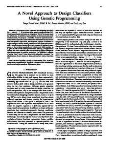
PSOs (both the hand-designed and the extended ones) are much less efficient. The fact that PSODISP2 is very good on Rastrigin problems even though it has been evolved on the city-block sphere class, suggests that this XPS could be a good all-rounder. It is interesting to compare the dynamic behaviour of the best PSOs found. In particular, the figures visually compare the behaviour of the swarm and how the dispersion of the swarm around the centre of mass varies in time for two XPSOs, PSOG3 and PSODISP2, together with the standard PSO, for the Rastrigin class of problems with dimension N = 2 and global optimum in the origin. PSO (figure 1) and PSODISP2 (figure 2) show typical behaviour for efficient PSOs, with particle trajectories rapidly converging to a tight symmetric spiral around the global optimum, with PSODISP2 doing so more efficiently. It seems that the dispersion term ensures that the swarm remains in a denser cloud. PSOG3 (figure 3) behaves differently: the particles still converge rapidly, but to a point slightly away from the optimum. This is still close enough to ensure good GP fitness values. However the swarm best converges to the optimum better than all the others, as table 2 confirms.
1. apply the approach to a variety of real-world problems 2. extend the approach by allowing GP to use more information on the past history of the swarm to control the particles 3. explore the effects and benefits of using different performance measures for PSO evolution.
174
All PSO particles
All PSO particle best
4
4
2
2
0
0
-2
-2
(a)
(b)
-4
-4
-2
-4
0
2
4
-2
-4
2
0
2
4
3.5 Swarm best Swarm center
Swarm dispersion
1.5
3
1 2.5 0.5 2 0 1.5 -0.5 1
(c)
-1
(d)
0.5
-1.5
-2
0 -2
-1.5
-1
-0.5
0
0.5
1
1.5
2
0
5
10
15
20
25
30
Figure 1: Prototypical run of PSO on the Rastrigin problem of dimension N = 2 showing, from top to bottom: (a) Trajectories of the particles, (b) Trajectories of the particle bests, (c) Trajectories of the swarm bests and of the centre of mass of the swarm, (d) Dispersion of the swarm around the centre of mass
All PSO particles
All PSO particle best
4
4
2
2
0
0
-2
-2
(a)
(b)
-4
-4
-4
-2
0
2
4
-4
2
-2
0
2
4
3.5 Swarm best Swarm center
Swarm dispersion
1.5
3
1 2.5 0.5 2 0 1.5 -0.5 1
(c)
-1
(d)
0.5
-1.5
-2
0 -2
-1.5
-1
-0.5
0
0.5
1
1.5
2
0
5
10
15
20
25
30
Figure 2: Prototypical run of PSODISP2 on the Rastrigin problem of dimension N = 2 showing, from top to bottom: (a) Trajectories of the particles, (b) Trajectories of the particle bests, (c) Trajectories of the swarm bests and of the centre of mass of the swarm, (d) Dispersion of the swarm around the centre of mass
175
All PSO particles
All PSO particle best
4
4
2
2
0
0
-2
-2
(a)
(b)
-4
-4
-4
-2
0
2
4
-4
2
-2
0
2
4
3.5 Swarm best Swarm center
Swarm dispersion
1.5
3
1 2.5 0.5 2 0 1.5 -0.5 1
(c)
-1
(d)
0.5
-1.5
-2
0 -2
-1.5
-1
-0.5
0
0.5
1
1.5
2
0
5
10
15
20
25
30
Figure 3: Prototypical run of PSOG3 on the Rastrigin problem of dimension N = 2 showing, from top to bottom: (a) Trajectories of the particles, (b) Trajectories of the particle bests, (c) Trajectories of the swarm bests and of the centre of mass of the swarm, (d) Dispersion of the swarm around the centre of mass
7.
ACKNOWLEDGMENTS
[10] J. Kennedy and R.C. Eberhart, Particle Swarm Optimization, IEEE ICNN, 1942-1948, 1995. [11] J.R. Koza, Genetic Programming, MIT Press, 1992. [12] T. Krink, J.S. Vesterstrøm, and R. Riget, Particle Swarm Optimisation with Spatial Particle Extension, CEC, 1474-1479, 2002. [13] W.B. Langdon and R. Poli, Foundations of Genetic Programming, Springer-Verlag, 2002. [14] M. Løvbjerg and T. Krink, Extending Particle Swarms with Self-Organized Criticality, CEC, 1588-1593, 2002. [15] E. Ozcan and C.K. Mohan, Particle Swarm Optimization: Surfing the Waves, CEC, 1939–1944, 1999. [16] R. Poli and C.R. Stephens, Constrained Molecular Dynamics as a Search and Optimization Tool, EuroGP, 150-161, 2004. [17] R. Poli,W.B. Langdon and O. Holland, Extending Particle Swarm Optimisation via Genetic Programming, EuroGP, 291-300, 2005. [18] Y. Shi and R.C. Eberhart, A Modified Particle Swarm Optimizer, CEC, 69–73, 1999. [19] J.S. Vesterstrøm, J. Riget and T. Krink, Division of Labor in Particle Swarm Optimisation, CEC, 1570-1575, 2002. [20] D. Wolpert and W.G. Macready, No Free Lunch Theorems for Optimization, IEEE Trans. Evolutionary Computation, 1, 1, 67-82, 1997.
The authors would like to thank EPSRC (grant GR/T11234/01) for financial support. We would also like to thank Owen Holland, Chris Stephens and Thiemo Krink for their comments.
8.
REFERENCES
[1] P.J. Angeline, Using Selection to Improve Particle Swarm Optimization, ICEC, 84–89, 1998. [2] W. Banzhaf, P. Nordin, R.E. Keller and F.D. Francone, Genetic Programming: an Introduction, Morgan Kaufmann Publishers, 1998. [3] T.M. Blackwell and P.J. Bentley, Dynamic Search with Charged Swarms, GECCO, 19–26, 2002. [4] T.M. Blackwell and J. Branke, Multi-swarm Optimization in Dynamic Environments., EvoWorkshops, 489-500, 2004. [5] E. Bonabeau, M. Dorigo and G. Theraulaz, Swarm Intelligence: from Natural to Artificial Systems, Oxford University Press, 1999. [6] R. Brits, A.P. Engelbrecht and B. Bergh, A Niching Particle Swarm Optimizer, SEAL, 692–696, 2002. [7] M. Clerc and J. Kennedy, The Particle Swarm Explosion, Stability, and Convergence in a Multidimensional Complex Space, IEEE Trans. Evolutionary Computation, 6, 1, 58-73, 2002. [8] J. Kennedy, The Behavior of Particles, Evolutionary Programming, 581-589, 1998. [9] J. Kennedy and R.C. Eberhart, Swarm Intelligence, Morgan Kaufmann Publishers, 2001.
176