Fast Incremental Learning for One-class Support Vector ... - CiteSeerX

Fast Incremental Learning for One-class Support Vector Classifier using Sample Margin Information Pyo Jae Kim Hyung Jin Chang Jin Young Choi EECS Department, Automation and System Research Institute (ASRI) Seoul National University, Seoul, Korea {pjkim,hjchang,jychoi}@neuro.snu.ac.kr Abstract In this paper, we present a fast incremental one-class classifier algorithm for large scale problems. The proposed method reduces space and time complexities by reducing training set size during the training procedure using a criterion based on sample margin. After introducing the sample margin concept, we present the proposed algorithm and apply it to face detection database to show its efficiency and validity.

1. Introduction Abnormality detection tasks, such as machine fault detection, medical diagnostic, and network intrusion detection, need different approaches from the conventional pattern classification or regression methods [1]. These problems are called one-class classification problems. The aim of these classification problems is to decide whether a data is in target class or not. One-class SVCs are the extended version of the original support vector machine (SVM) to one-class problems. Well-known one-class SVCs are one-class SVM [2] and Support Vector Data Description (SVDD) [3]. These batch type one-class SVCs are formalized to similar dual problems and solve using quadratic programming (QP) method. Although QP solver, which is used for finding Lagrange multipliers α, has an advantage of avoiding a local minimum problem, it needs O(n3 ) time and O(n2 ) spatial complexities. In general, incremental learning, as opposed to batch learning in which all data are available at once, assumes that one training data is presented at a time and updates all weights whenever a new data is added. Cauwenberghs et al. [4] developed an incremental support vector machine (SVM) giving almost similar solution with the optimal one gotten by a batch learning. Some use-

978-1-4244-2175-6/08/$25.00 ©2008 IEEE

ful implementation issues on incremental SVM are presented in [5]. However there is no explicit version of incremental one class SVC. Although the incremental learning of one-class SVC can reduce the computational complexity by avoiding QP, it still suffers from scale problems on a large scale problem for their iterative learning process. Moreover, because it stores all trained data to get an optimal solution, computational complexity and data storage space keep increase as learning process goes on. To solve this problem, we review the geometric interpretation and propose sample margin concept. Using this sample margin, we add a process, which removes non support vectors (NSVs), to incrental SVC algorithm that the proposed method can deal with very large scale data with low spacial and computational complexity. In addition, we derive the framework of incremental SVC following the results in [4], [5], and propose a fast incremental learning mothod using sample margin information. The experiment shows that the presented method can make incremental SVC deal with very large data set with low spatial and computational complexity.

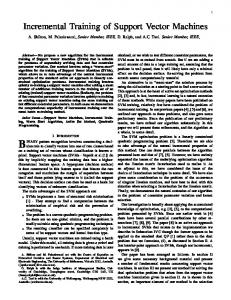
2. Geometric Interpretation of Two Oneclass SVCs As shown in Fig. 1, the norm of center of SVDD [3] is equal to the margin of hyperplane of one-class SVM [2]. The segment intersecting the unit hypersphere, on which all data live, with the hyperplane of one-class SVM is just like the hypersphere of SVDD. So the two SVCs give identical solutions in the unit normed feature space. In the unit norm feature space, the hypersphere of SVDD can be reformulated by the new hyperplane equation like that of one-class SVM. φ(x) − a2 ≤ R2

⇐⇒

wsvdd · φ(x) − ρsvdd ≥ 0, (1)

One-class SVM SVDD

R

O

O

Feature space

Figure 1. Geometric relation between one-class SVM and SVDD. The margin of hyperplane of two one-class SVC is ρ γone-class svm = w , γsvdd = a for each.

Figure 2. Definition of sample margin γ(x) for data x in SVDD. Sample margin is the distance from the image of data φ(x) to a the virtual hyperplane a · φ(x) = 0.

where a is the hypersphere center of SVDD. The normal vector wsvdd and the bias ρsvdd of SVDD hyperplane is as below: a , ρsvdd = a. wsvdd = (2) a

3. Sample Margin Sample margin is defined by the distance from the image of data x to the virtual hyperplane which passes through the origin of feature space and parallels to the optimal hyperplane as shown in Fig. 2. In SVDD, sample margin is defined as below: a · φ(x) γsvdd (x) = , a

(3)

where a is the center of SVDD’s hypersphere and φ(x) is the image of data x in feature space. In one-class SVM, sample margin is defined as follows: γonc-class svm (x) =

w · φ(x) . w

(4)

Because data examples exist on the surface of unit hypersphere, the sample margin has 0 as the minimum value and 1 as the maximum, i.e. 0 ≤ γ(x) ≤ 1.

(5)

Also, sample margins of unbounded support vectors 1 xUSV (0 < αxU SV < νn ) are the same as the margin of hyperplane. So γ(xUSV ) = γsvdd = a, γ(xUSV ) = γone-class svm =

ρ . w

(6) (7)

O

Feature space

Input space

Figure 3. Data distribution in feature space and date description boundary in input space. The data on same contour in input space have same sample margins.

Sample margin represents the distribution of images of data in feature space. The left figure of Fig. 3 shows the distribution of sample margin of training data and hyperplane of one-class SVC in feature space.

4. Incremental SVC using Sample Margin Information 4.1. Incremental SVC The trained data are partitioned into three categories based on the Kuhn-Tucker condition [8]: the set S denotes margin support vectors (or USVs, 0 < αi < C), the set E denotes error support vectors (or BSVs, αi = C) and the set R denotes NSVs which are within a data description (or NSVs, αi = 0). We shall use lower-case letters ‘s’, ‘e’, and ‘r’ for each partitions respectively. The lower-case letter ‘c’ represents a newly added data at present. The Kuhn-Tucker conditions have to be maintained for all trained data before a new data xc is added. These conditions are also preserved after the new data

Figure 5. The candidates of removable NSV and  region.

Figure 4. The overall scheme of incremental learning method for one-class SVC. is trained. That is, the change of Lagrange multipliers (Δα) is determined to hold the Kuhn-Tucker conditions. In general, the Lagrange multipliers of BSVs and NSVs do not vary during each update step. Only the Lagrange multipliers of USVs and newly added data xc change their value to satisfy the Kuhn-Tucker conditions during a update process. In the incremental SVC algorithm, the update process of incremental support vector learning is done by two simple linear relations and controlled by the increment Δαc of newly added data xc . Therefore the most important task is to determine the increment Δαc . To account for the movement of some data from one set to the other during the update process, we should determine the largest possible increment Δαc so that the composition of these set remains intact. For this purpose, five cases must be considered. The overall flow chart of incremental SVC is shown in Fig. 4.

4.2 Complexity Reduction Method based on Sample Margin The computational complexity of incremental method is also proportional to the number of data so the increment of data size causes scale problems in incremental support vector learning. The spatial complexity is even more serious because all trained data have to be preserved. To make incremental support vector learning more scalable in a real large problem, we need to remove useless data. In our approach, we propose a novel complexity reduction method by removing useless data based on the sample margin defined in chapter 3. Incremental learning of one-class SVC is a method finding a decision boundary considering only data trained up to present. Because all data are not trained, the current data description is not optimal for whole

data set but it can be considered as an optimal data description for trained data up to now. We can eliminate every NSVs classified by the current hyperplane. However it is risky because important data which have a chance to be unbounded support vectors (USVs) might be removed as learning proceeds incrementally so the current hyperplane may not converge on the optimal hyperplane. Therefore we need to define cautiously removable NSVs using sample margin. To handle the problem of removing data which become USVs, we choose data whose sample margin is in the specific range as removable NSVs. As shown in Fig. 5, we intend to select data in the region above the gray zone as removable NSVs. The gray region called  region is defined to preserve data which may become USVs. The removable NSV is defined as follows: Definition 4.1 (The candidate of removable NSV). The data xi which meets the following condition, is the candidate of removable NSV. γ(x) − γ(xUSV ) ≥ , γmax − γ(xUSV )

(8)

where  is the user defined coefficient and selected in the range of 0 <  ≤ 1, γ(xUSV ) is the sample margin of USV which is on the data description boundary, and γmax = maxi∈R γ(xi ). As in Fig. 5, by preserving data in  region, a novel incremental SVC using sample margin information can obtain the same data description as original incremental SVC with less computational and spatial load. If  is ‘0’, then we assume all data lying on the upper side of hyperplane as the candidates of removable non support vectors, and this makes learning unstable. When  is ‘1’, we can hardly select removable NSVs, so the effect of speeding up and storage reduction is meager.

5. Experiments The following experiment was performed for comparison on training time, required storage space and accuracy between the proposed algorithm and the existing algorithms. We used Tax’s data description toolbox

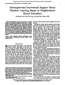
tween multi-class SVMs and the proposed method decreases as shown in Fig. 6. Fig. 6 represents the incremental capability of the proposed method. That is, the accuracy of the proposed method increases as the learning goes on.

100 95

Accuracy (%)

90 85 80 75 70

6. Conclusion

65 60

0

500

1000

1500

2000

2500

3000

3500

# of trained data

Figure 6. Incremental learning capability of the proposed method for face detection database. Table 1. Experimental results on face detection database Results are averaged over 10 runs.  of the proposed method is 0.45. Method

Accuracy (%) OAA 91.5 OAO 91.5 IncSVDD 87.5 Proposed 87.5 method

Training time (s) 416.80 209.73 27.19 3.58

# of SVs 582 291 50 50

# of stored data 1500 1500 1500 118

[9]. Simulations were run on a PC with a 3.0 GHz Intel Pentium IV processor and 1G RAM. We used quadratic program solver (quadprog) provided by MATLAB for batch methods using QP solver.

5.1. Face Detection Database To test the scale problem, we used the face detection database [10] as a real large face recognition problem. This database consists of two types of images representing face and non-face respectively. Each image has 24×24 dimensions. The number of face database is 4916 and that of non-face database is 7872. Because this problem was binary classification problem, multi-class SVMs such as One-Against-All(OAA) and One-Against-One(OAO) were used. Moreover, because the computational load of multi-class SVM is extremely massive when the number of data is over 2000, we used 1500 data among a training set. Table 1 shows the classification accuracies, training time and required storage space of all tested methods. Although the classification performance of the proposed method was a little lower than multi-class SVMs, the proposed method needed the smallest training time and storage space. If learning goes forward over 1500 data, the difference of training accuracy be-

In this paper we dealt with a scale problem of incremental SVC. By adopting incremental SVM learning framework, incremental learning of one-class SVC can avoid QP. However as the number of data to be learned increases, it also suffers from scale problems. To solve this, we proposed sample margin information. By removing data which have high probability to become NSVs which are selected by sample margin information, we could save computational time and storage space. From the experiment using real large data, we showed improvement in computation load and storage space of the proposed method.

References [1] M. Moya, M. Koch, and L. Hostetler, “One-class classifier networks for target recognition applications,” in Proc. world congress on neural networks, pp. 797-801, 1993. [2] B. Sch¨olkopf, J. Platt, J. Shawe-Taylor, A. J. Smola, and R. C. Williamson, “Estimating the support of a highdimensional distribution,” Neural Computation, vol. 13, no. 7, pp. 1443-1471, 2001. [3] D. M. J. Tax, R. P. W. Duin, “Support Vector Data Description,” Machine Learning, vol 54, pp. 45-56, 2004. [4] G. Cauwenberghs and T. Poggio, “Incremental and decremental support vector machine learning,” Neural Information Processing Systems, pp. 409-415, 2000. [5] P. Laskov, C. Gehl, S. Kr¨uger, and K. R. M¨uller, “Incremental support vector learning: Analysis, Implementation, and Applications,” Journal of Machine Learning Research, vol 7, pp. 1909-1936, 2006. [6] B. Sch¨olkopf, A. Smola, R. C. Williamson, and P. L. Bartlett, “New support vector algorithms,” Neural Computation, vol. 12, no. 5, pp. 1207-1245, 2000. [7] D. M. J. Tax and P. Laskov, “Online SVM learning: From classification to data description and back,” IEEE XIII Workshop on Neural Networks for Signal Processing, pp. 499-508, 2003. [8] M. Pontil, and A. Verri, “Properties of support vector machines,” Neural Computation, vol. 10, pp. 995-974, 1997. [9] D. M. J. Tax, DDtools, “the Data Description Toolbox for Matlab,” http://wwwict.ewi.tudelft.nl/∼ddavidt/dd tools.html, 2006. [10] Face detection database, http://www.cs.ubc.ca/∼pcarbo/#code,