sensors Article
Fault Diagnosis from Raw Sensor Data Using Deep Neural Networks Considering Temporal Coherence Ran Zhang 1,2,3 , Zhen Peng 4 , Lifeng Wu 1,2,3, *, Beibei Yao 1,2,3 and Yong Guan 1,2,3 1 2 3 4
*
College of Information Engineering, Capital Normal University, Beijing 100048, China;
[email protected] (R.Z.);
[email protected] (B.Y.);
[email protected] (Y.G.) Beijing Engineering Research Center of High Reliable Embedded System, Capital Normal University, Beijing 100048, China Beijing Advanced Innovation Center for Imaging Technology, Capital Normal University, Beijing 100048, China Information Management Department, Beijing Institute of Petrochemical Technology, Beijing 102617, China;
[email protected] Correspondence:
[email protected]; Tel.: +86-134-0110-8644
Academic Editor: Vittorio M. N. Passaro Received: 14 January 2017; Accepted: 7 March 2017; Published: 9 March 2017
Abstract: Intelligent condition monitoring and fault diagnosis by analyzing the sensor data can assure the safety of machinery. Conventional fault diagnosis and classification methods usually implement pretreatments to decrease noise and extract some time domain or frequency domain features from raw time series sensor data. Then, some classifiers are utilized to make diagnosis. However, these conventional fault diagnosis approaches suffer from the expertise of feature selection and they do not consider the temporal coherence of time series data. This paper proposes a fault diagnosis model based on Deep Neural Networks (DNN). The model can directly recognize raw time series sensor data without feature selection and signal processing. It also takes advantage of the temporal coherence of the data. Firstly, raw time series training data collected by sensors are used to train the DNN until the cost function of DNN gets the minimal value; Secondly, test data are used to test the classification accuracy of the DNN on local time series data. Finally, fault diagnosis considering temporal coherence with former time series data is implemented. Experimental results show that the classification accuracy of bearing faults can get 100%. The proposed fault diagnosis approach is effective in recognizing the type of bearing faults. Keywords: faults diagnosis; deep neural networks; raw sensor data; temporal coherence
1. Introduction Monitoring machinery health conditions is crucial to its normal operation. Recognizing the deficiencies of machinery contributes to the control of the overall situation. Fault diagnosis models based on data-driven methods are a great advantage since that they require no physical expertise and provide accurate and quick diagnosis from data which are easily obtained by sensors. Traditional data-driven fault diagnosis models are usually based on signal processing methods and some classification algorithms. Signal processing methods are mainly used to decrease noise and extract features from the raw data. In this field, time domain feature methods [1–3], including Kernel Density Estimation (KDE), Root Mean Square (RMS), Crest factor, Crest-Crest Value and Kurtosis, frequency domain features [4] such as the frequency spectrum generated by Fourier transformation, time-frequency features obtained by Wavelet Packet Transform (WPT) [5] are usually extracted as the gauge of the next process. Other signal processing methods such as Empirical Mode Decomposition (EMD) [6], Intrinsic Mode Function (IMF), Discrete Wavelet Transform (DWT), Hilbert Huang
Sensors 2017, 17, 549; doi:10.3390/s17030549
www.mdpi.com/journal/sensors
Sensors 2017, 17, 549
2 of 17
Transform (HHT) [7,8], Wavelet Transform (WT) [9] and Principal Component analysis (PCA) [10] are also implemented for signal processing. These signal processing and feature extraction methods are followed by some classification algorithms including Support Vector Machine (SVM), Artificial Neural Networks (ANN), Wavelet Neural Networks (WNN) [11], dynamic neural networks and fuzzy inference. These classification algorithms are usually used to recognize faults according to the extracted features. Yu et al. [7] used Window Marginal Spectrum Clustering (WMSC) to select features from the marginal spectrum vibration signals by HTT and adopted SVM to classify faults. Wang et al. [8] used the statistical locally linear embedding algorithm to extract low dimensional features from high dimensional features which are extracted by time domain, frequency domain and EMD methods. Regression trees, K-nearest-neighbor classifier and SVM were adopted as the classifiers, respectively. Li et al. [12] used Gaussian-Bernoulli Deep Boltzmann Machine (GDBM) to learn from statistical features of time domain, frequency domain and time-frequency domain. GDBM was also taken as the classifier. Cerrada et al. [13] used a multi-stage feature selection mechanism to select best set of features for the classifier. These researches focus on the steps of feature extraction and selection. However, these fault diagnosis approaches suffer from some drawbacks. Firstly, applying noise decreasing and feature extraction methods to practical issues properly requires specific signal processing expertise. Specific circumstances call for specific signal processing methods which depend on signal and mathematics expertise; Secondly, the performances of these classifiers completely depend on the features which are extracted from time series signals. Although appropriate features help the decision and recognition, ambiguous features will mislead the model. Thirdly, the feature extraction methods will definitely lose some information such as the temporal coherence of time series data which cannot be ignored. This paper presents a novel model based on DNN to recognize the raw sensor signals, which are time series data. It has been proved that Deep Learning [14], or Deep Neural Networks are able to reduce the dimensionality and learn characteristics from nonlinear data in the fields of image classification [15], speech recognition [16] and sentiment classification [17]. There are great advantages in the fact that the model can learn directly from the raw time series data and make use of the temporal coherence. The merits of the proposed model are as follows: (1) pretreatments such as noise decreasing and specific time domain and frequency domain feature extraction methods are not needed since the proposed model is competent for the task of learning characteristics from raw time domain signals adaptively; (2) the temporal coherence of time series data is taken into consideration in the proposed model; (3) the proposed model is a supervised learning model and has great abilities of generalization and recognition for the normal and faults data. The classification accuracy on bearing vibration datasets can be 100%. Complex models are capable of generalizing well from raw data so data pretreatment(s) can be omitted. Models with simple structure do not perform as well as those with deeper and more complex structures, but they are easy to train because they need less parameters. Complex models can get a better understanding of the data due to their multitude of units and layers, however, complex models do not always perform better than simple models. This paper also discusses how the structure of the model affects the performance. In order to clearly illustrate the model and their performance, the rest of this paper is grouped together as follows: Section 2 describes the details of the proposed fault diagnosis model. Section 3 describes our experiments and results. Section 4 discusses some details of the model structure and makes some comparisons with traditional methods. Section 5 draws the conclusions. 2. Methods This paper presents a fault diagnosis model based on DNN to recognize defects. Inputs of DNN are raw time domain data instead of time domain or frequency domain features. Outputs are the targets, i.e., the categories of data. A deep neural networks structure model is used to learn
Sensors 2017, 17, 549
3 of 17
local characteristics adaptively from the raw time series data. Then temporal coherence is taken into 3 of 17 make a diagnosis.
Sensors 2017, 17, 549 consideration to
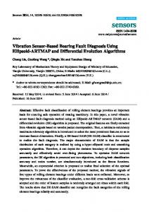
2.1. Structure Structure of of Proposed Proposed Fault Fault Diagnosis Diagnosis Model 2.1. As shown shownininFigure Figure1,1,segments segments time series data used as training testing samples. As ofof time series data areare used as training and and testing samples. The The size of the segment is set to be a fixed value and it is also the input size of a deep neural networks. size of the segment is set to be a fixed value and it is also the input size of a deep neural networks. The data data from from time time t1 t1 to to t2 t2 are are taken taken as as inputs inputs to tothe theproposed proposed model model and and the the size size of ofthe thesegmentation segmentation The is t2 t2 −−t1.t1.InIn this way, continuous dimensional series is divided into segments. is this way, thethe continuous oneone dimensional timetime series datadata is divided into segments. The The time memory is other n, in other words, n is the number of outputs of y(t) DNN y(t) is which is temporarily time memory is n, in words, n is the number of outputs of DNN which temporarily stored stored fault diagnosis considering temporal coherence. Therefore, first output of proposed for faultfor diagnosis considering temporal coherence. Therefore, the firstthe output of proposed model model is which is denoted is at − t1).for Then, forsingle everylength singletime, length time,iswhich is which denoted as Y(n) as is Y(n) at time n time × (t2 n− × t1).(t2Then, every which t2 − t1, t2 − t1, there is an Y(t). output For the simplification of representations, Y(t) denotes the final output there is an output ForY(t). the simplification of representations, Y(t) denotes the final output of the of the proposed time this article. proposed model model at timeatt in restt in of rest this of article.
Figure Figure 1. 1. The Thestructure structure of of proposed proposed fault fault diagnosis diagnosis model. model.
The modelisisbased basedononthe the deep structure of neural networks. A logistic function is The proposed proposed model deep structure of neural networks. A logistic function is used used as the activation function among input layers and hidden layers. For every segmentation, the as the activation function among input layers and hidden layers. For every segmentation, the model model could set of values. output Time values. Time memory is set to record values of output could get a setget of aoutput memory is set to record values of output value y(t). value Thesey(t). sets These sets of former outputs of DNN values are gathered to get final outputs of time considering of former outputs of DNN values are gathered to get final outputs of time considering model via model via linear transformation: linear transformation: 1 nn Y (t) = 1 ∑ λ T y(t − T ) (1) Y(t ) = n T (1) =0λT y(t T ) n T =0 In the above equation, Y(t) is the final outputs at current time and y(t) is the outputs of DNN at In the above Y(t)connecting is the finalthe outputs at units current time and thefinal outputs of DNN current time. λ is equation, the weights output of DNN y(t)y(t) andisthe output units at of the nweights connecting the output of DNN y(t) andmodel the final output of current time. isY(t). proposed model is the number of DNN outputsunits which the proposed takes into units account. proposed Y(t). n is as thethe number of DNN outputs which the proposed model takes into account. It can alsomodel be considered time length. It can also be considered as the time length.
Sensors 2017, 17, 549
4 of 17
2.2. Deep Neural Networks Deep learning is firstly introduced in image classification [18] and it is used to reduce the dimensionality of data and recognize images. Deep Learning, or DNN can learn some useful features from the data adaptively without expertise in specific fields. It has received extensive attention in the fields concerned with nonlinear mapping. DNN is a model of stacked layers of units which are connected layer by layer and there is no connection among the units in the same layer. There are an input layer and an output layer in the model. Also, a few hidden layers are placed between the input layer and output layer. The number of input layer units and output layer units are set according to the dimensionalities of the input data and the target data, respectively. However, there are no strict rules for the settings of the number of every hidden layer’s units. There are nonlinear relationships between the adjacent layers. They are defined as follows: m am (2) j = σ(z j ) zm j =
∑ wij aim−1 + bmj
(3)
i
m where am j is the activation of neural j in layer m, z j is the sum of bias and linear combination of former activations, bm j is the biases vector of neural j in layer m. w ji is the weight matrix between layer i and layer j, σ (z) is the activation function and there are a few kinds of this function as follows:
σ(z) = 1/(e−z + 1) σ(z) =
ez − e−z ez + e−z
σ(z) = max (0, z)
(4) (5) (6)
Equation (3) is a logistic function and this is mostly used in DNNs. Equation (4) is called the tanh function. The range of output values are from −1 to 1. It is different from the logistic function which is easier to implement in the DNNs sometimes. Equation (5) represents rectified linear units (ReLU). Its output is always positive. In this paper, the logistic function are used as the activation function. Every unit in the next layer is connected to all units in the formal layer. The activation units of input layer are the input data while output units of last layer are targets. W and b are the parameters of the model and they are randomly initialized. Thus, the outputs y can be calculated layer by layer given the input data x and the model’s parameters: a1 = x
(7)
m −1 −1 am + bm ), j > 1 j = σ ( ∑ wij ai j
(8)
y = aM
(9)
i
where M is the number of layers in the network. The inputs of first layer a1 are the inputs of DNN. The outputs of last layer a M are defined as the outputs of DNN. The error can be worked out by contrasting the calculated outputs y with targets t: C (t, y) =
1 ∑ ( t i − y i )2 k∑ k i
(10)
where C is the cost function, k is the number of training samples and i represents the dimension of y and t. The cost function is used to measure the error and the usual form is squared reconstruction error. The aim of training DNN is to minimize the cost function, in other words, to make the error of
Sensors 2017, 17, 549
5 of 17
outputs close or equal to zero. To minimize it, a gradient descent algorithm is utilized and the gradient is calculated as follows: ∂C ∂C ∂C , , ..., ) (11) ∇C = ( ∂θ1 ∂θ1 ∂θ N In the equation, θ represents parameters including the weights and biases of the layers in DNN model and the total number of parameters is N. Partial derivatives of weights and biases of last layer are first calculated according to the error in the last layer. Then the error is back propagated to former layers and all the partial derivatives are worked out. Once the gradient is computed, parameters are updated by the following rules: ∂C w = w+η (12) ∂w b = b+η
∂C ∂b
(13)
In the equation, η is the learning rate. The process of computing gradient and updating parameters is in an epoch. The epochs can either be set to a fixed number or adjusted according to the performance of networks. We train the networks and fine tune the parameters over and over again until the error of the network has declined to the minimum value. 2.3. Cross Entropy Cost Function and Partial Derivations When training neural networks, gradient descent and back propagation algorithms are utilized. Gradients can be calculated by the partial derivative of the cost function for parameters such as weights and biases. Traditional work chooses the squared reconstruction error (Equation (9)) as cost function. However, in the training process of deep neural networks, this will lead to a saturation problem [19]. In other words, all the partial derivatives will be close to zero so the parameter updating will be slow before the networks achieve the best performance. When the cross entropy, also known as Kullback-Leibler (K-L) divergence, is chosen as cost function, the saturation problem will be avoid. In the proposed model, cross entropy is taken as the cost function to compute the errors. The dimension of inputs, i.e., the number of input neurons is determined by the size of the inputs data and the outputs dimension equals to the number of data types. The cross entropy cost function is defined as follows: 1 C (t, y) = − ∑ ∑ [ti lnyi + (1 − ti )ln(1 − yi )] (14) k k i where t are targets, y are the outputs of the model, k is the number of training samples. The main purpose of training is to minimize the cost function. It is obviously that when the outputs y are close to the targets t, the value of cost will be close to zero. Also the value of the cross entropy cost function will always be positive. These two properties are fundamental for a proper cost function. A gradient descent is used to minimize the cost function, so the partial derivations are calculated as follows: ∂C = aim−1 em (15) j ∂wijm ∂C = em j ∂bm j eim =
(16)
∑ wijm+1 emj +1 σ0 (zim )
(17)
∑ (t j − y j )
(18)
j
e jM =
k
where k is the number of training samples, layer M is the last hidden layer. em j is the error of neural j in layer m, t are the targets. aim−1 is the activation value of neural i in layer m − 1. wijm represents the weight from neural i in layer m − 1 to neural j in layer m. While the error is back propagated
e jM = (t j y j ) k
(178 )
where k is the number of training samples, layer M is the last hidden layer. ݁ is the error of neural 2017, 17, 549 6 of 17 jSensors in layer m, t are the targets. aim 1 is the activation value of neural i in layer m − 1. ݓ represents
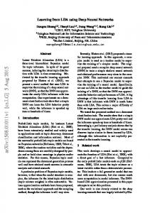
the weight from neural i in layer m − 1 to neural j in layer m. While the error is back propagated to to the former layer, partial derivationsofofweights weightsand andbiases biasesare arecalculated calculatedlayer layerby by layer layer so so the the former layer, thethe partial derivations parameters can be updated. 2.4. Training Training of 2.4. of DNN DNN and and Fault Fault Diagnosis Diagnosis Steps Steps The flow flow chart chart of The of the the proposed proposed fault fault diagnosis diagnosis approach approach is is shown shown in in Figure Figure 2. 2.
Figure Figure 2. 2. Flowchart Flowchart of of the the proposed proposed fault fault diagnosis diagnosis approach. approach.
Firstly, the DNN model is trained using historic data and the time memory of the model is set Firstly, the DNN model is trained using historic data and the time memory of the model is set to 0. to 0. That is to say, the output of DNN is used as the output of the whole model. In the training That is to say, the output of DNN is used as the output of the whole model. In the training process, the process, the time coherence is not utilized so the DNN can independently learn the local time coherence is not utilized so the DNN can independently learn the local characteristics from local characteristics from local vibration data. In this way, the current segmentation will not have any effect vibration data. In this way, the current segmentation will not have any effect of adjacent segments, of adjacent segments, which is helpful to train a better model. After the training processes come the which is helpful to train a better model. After the training processes come the testing process and fault testing process and fault recognition process. The test data are used to test the classification ability of recognition process. The test data are used to test the classification ability of the trained DNN without the trained DNN without considering temporal coherence. In the fault recognition process, the considering temporal coherence. In the fault recognition process, the temporal coherence is taken into temporal coherence is taken into consideration. The output Y(t) of proposed model at current time consideration. The output Y(t) of proposed model at current time can be computed by the current output of DNN y(t) and the former outputs y(t − n) to y(t − 1) which were stored for a specific time period. The detailed training steps are as follows: (a)
Set the size of segmentation and divide the time series data into segments.
Sensors 2017, 17, 549
7 of 17
by the current output of DNN y(t) and the former outputs y(t − n) to y(t − 1) which 7 of 17 were stored for a specific time period. The detailed training steps are as follows:
can be2017, computed Sensors 17, 549
(a) Set the size initialize of segmentation and divide the time series data into and segments. (b) Randomly the parameters of DNN including weights biases of every hidden and (b) Randomly initialize the parameters of DNN including weights and biases of every hidden and output layer. (c) output Select alayer. group of segments as DNN inputs. (c) Select a group of segments DNN inputs. (d) Compute the activations ofas every layer according to the input raw data, weights, biases. (d) Compute the activations of every layer according to the input raw data, weights, biases. (e) Cross entropy is used to compute the error of outputs compared to targets. (e) Cross entropy is used to compute the error of outputs compared to targets. (f) Use the back propagation algorithm to compute the error of every layer and the gradients (f) Use the back propagation algorithm to compute the error of every layer and the gradients of of parameters. parameters. (g) Update parameters with the gradients and learning rate. (g) Update parameters with the gradients and learning rate. (h) Repeatsteps steps (c) (c) to to (g) (g) until until the the error error of of outputs outputs reach reach the the minimum minimum value. value. (h) Repeat The Thedetailed detailedfault faultrecognition recognitionsteps stepsare areas asfollows. follows.
(a) (a) (b) (b)
(c) (c) (d) (d) (e) (e)
Set . Setthe themodel’s model’s memory memory length length nn and and connection connection weights weights λ. and the the size size of of segmentation segmentation is is s,s, Divide Dividethe the time time series series data data into into segments. segments. IfIf current current time time is is tt and the segmentation t are sample points from t − s to t and segmentation t − n are sample points from the segmentation t are sample points from t − s to t and segmentation t − n are sample points tfrom − (n +t − 1) (n × s+to1)t × − ns ×tos.t − n × s. Compute the outputs y(t − n) to y(t) of DNN using segmentation t − n to segmentation t as inputs Compute the outputs y(t − n) to y(t) of DNN using segmentation t − n to segmentation t as and store them. inputs and store them. Compute Y(t) using outputs of DNN from y(t − n) to y(t) and recognize the data. Compute Y(t) using outputs of DNN from y(t − n) to y(t) and recognize the data. When new time series data is available, make them new segments and compute the DNN output. When new time series data is available, make them new segments and compute the DNN output. Then, compute the outputs of the proposed model which considers the DNN output history. Then, compute the outputs of the proposed model which considers the DNN output history.
3. Experiments and Results 3. Experiments and Results
3.1. Intelligent IntelligentMaintenance MaintenanceSystem System(IMS) (IMS)Bearing BearingDataset Dataset 3.1. 3.1.1. Experimental ExperimentalApparatus Apparatusand andData DataCollection Collection 3.1.1. Inorder orderto tovalidate validatethe the proposed proposedmethod, method, experimental experimental data data are are applied applied to to test test its its performance. In Thedataset datasetisisprovided provided University of Cincinnati Center for Intelligent Maintenance Systems The byby thethe University of Cincinnati Center for Intelligent Maintenance Systems [20]. [20].experiment The experiment apparatus is shown in Figure 3. The apparatus is shown in Figure 3.
(a)
(b)
Figure 3. Experimental apparatus. (a) is the photo of bearings with sensors. (b) is the structure Figure 3. Experimental apparatus. (a) is the photo of bearings with sensors. (b) is the structure diagram diagram of apparatus. of apparatus.
As depicted in Figure 3, there was a shaft on which four bearings were installed. There were As depicted in Figure 3, two there was a shaft on four bearings were installed. There were eight accelerometers in total, accelerometers forwhich each bearing. The rotation speed of the shaft was eight accelerometers in total, two accelerometers for each bearing. The rotation speed of the shaft
Sensors Sensors 2017, 2017, 17, 17, 549 549
of 17 17 88 of
kept constant at 2000 revolutions per minute (RPM). It was driven by an alternating current (AC) was kept constant at 2000 revolutions per minute (RPM). It was driven by an alternating current (AC) motor which was connected to the shaft by friction belts. What’s more, there was a 6000 lbs radial motor which was connected to the shaft by friction belts. What’s more, there was a 6000 lbs radial load which was added to the bearings and shaft by a spring mechanism. All four bearings were force load which was added to the bearings and shaft by a spring mechanism. All four bearings were lubricated. The bearings were Rexnord ZA-2115 double row bearings. Accelerometers were installed force lubricated. The bearings were Rexnord ZA-2115 double row bearings. Accelerometers were on the bearing housing. The accelerometers were PCB 353B33 High Sensitivity Quartz ICPs. installed on the bearing housing. The accelerometers were PCB 353B33 High Sensitivity Quartz ICPs. Thermocouple sensors were placed on the bearings as shown in Figure 3. After rotating for more than Thermocouple sensors were placed on the bearings as shown in Figure 3. After rotating for more than 100 million revolutions, failures such as inner race defect, outer race failure and roller element defect 100 million revolutions, failures such as inner race defect, outer race failure and roller element defect occurred since the bearings worked for a long period which exceeded the designed life time. Data occurred since the bearings worked for a long period which exceeded the designed life time. Data were collected by a NI DAQ Card 6062E. The sampling rate was set as 20 kHz and every 20,480 data were collected by a NI DAQ Card 6062E. The sampling rate was set as 20 kHz and every 20,480 data points were recorded in a file. In every 5 or 10 min, the data were recorded and written in a file while points were recorded in a file. In every 5 or 10 min, the data were recorded and written in a file while the bearings were rotating. the bearings were rotating. 3.1.2. Data Segmentation 3.1.2. Data Segmentation Four kinds of data including normal data, inner race defect data, outer race defect data and roller Four kinds of data including normal data, inner race defect data, outer race defect data and roller defect data were selected. There are 20,480 data points in each file. For every kind of data, 20 files are defect data were selected. There are 20,480 data points in each file. For every kind of data, 20 files are chosen. It is too complex if they are directly used as the inputs of DNN since the data dimensionality chosen. It is too complex if they are directly used as the inputs of DNN since the data dimensionality is 20,480, so the data are cut into segments to form the samples. The sampling rate is 20 kHz and the is 20,480, so the data are cut into segments to form the samples. The sampling rate is 20 kHz and rotation speed is 2000 RPM, so it can be computed that the rotation period is 600 data points per the rotation speed is 2000 RPM, so it can be computed that the rotation period is 600 data points per revolution. The size of the segmentation is set to be a quarter of the rotation period, which is 150 data revolution. The size of the segmentation is set to be a quarter of the rotation period, which is 150 data points. Therefore, each file is separated into 136 segments. Then the total number of samples is 10,880 points. Therefore, each file is separated into 136 segments. Then the total number of samples is 10,880 with 150 data points in each segmentation. That is to say, there are 2720 samples for every kind of with 150 data points in each segmentation. That is to say, there are 2720 samples for every kind of data. Figure 4 shows an example of one rotation period of normal data and fault data. As we can see, data. Figure 4 shows an example of one rotation period of normal data and fault data. As we can the four kinds of data show in similar tendency and it is hard to classify them just by intuition, see, the four kinds of data show in similar tendency and it is hard to classify them just by intuition, therefore, some mathematical method(s) should be implemented for the recognition. A selected therefore, some mathematical method(s) should be implemented for the recognition. A selected dataset dataset description is shown in Table 1. description is shown in Table 1.
Figure 4. Four kinds of bearing vibration signals. (a) is the normal vibration data and the following three lines (b–d) are three kinds of fault data, inner race fault, outer outer race race fault fault and and roller roller defect, defect, respectively. The x axis represents time series and y axis represents the collected data value. respectively. represents time series and y axis represents the collected data value. Table 1. Description of selected IMS dataset. Data Type
Number of Samples
Label
Sensors 2017, 17, 549
9 of 17
Table 1. Description of selected IMS dataset. Data Type
Number of Samples
Label
Normal Inner race fault Outer race fault Roller defect
2720 2720 2720 2720
1 2 3 4
3.1.3. Training There are similar tendencies and features in the same kinds of data, which facilitates the classification of data. DNN has the capacity of learning the characteristics and similarities from raw time domain signals. The raw data collected by sensors are taken as inputs of the model and the outputs are data classifications. To select the best neural networks structure, DNN models with different structures are established. An upper bound of neurons is set. Before the training process, the dataset is divided into three parts: training dataset, testing dataset and validation dataset. The validation dataset is used to select the best trained neural network and to prevent overfitting. The testing dataset is used to calculate the classification accuracy of the networks. By training these supervised DNN models for hundreds of epochs, model parameters including weights and biases are adjusted to an expected value. In the meantime, the error of this model is decreased to the minimal value and the performance, which is measured by cross entropy, also reaches the expected level. Actually, cross entropy is directly related to errors between model outputs and targets. The cross entropy becomes less when model errors are decreased. The aim of training is to minimize the cross entropy. After training, the five layers model can get an accuracy of 94.4% on the test data when the temporal coherence is not taken into consideration. The simulation models are based on MATLAB. The CPU is an Intel(R) Core(TM) i7-4720HQ @ 2.60 GHZ (Intel Corporation, Santa Clare, CA, USA) and the computation time of the five layers model is 131.161 s for the whole training and testing process. Experimental results show that it can recognize the normal and fault data well, so the model attained good generalization ability. The classification accuracies of these models on the validation dataset (Val) and testing dataset (Test) are shown in Table 2. The confusion matrix of the best model on the testing dataset is shown in Table 3. Table 2. Classification accuracies of models with different layers.
Label
3 Layers Model
4 Layers Model
5 Layers Model
6 Layers Model
Val
Test
Val
Test
Val
Test
Val
Test
1 2 3 4
98.9% 92.3% 100% 93.0%
98.2% 92.6% 100% 84.9%
99.3% 91.9% 100% 90.8%
98.2% 91.5% 100% 85.7%
98.2% 93.8% 100% 91.9%
98.9% 91.5% 100% 87.1%
97.8% 90.1% 100% 87.9%
98.9% 90.8% 100% 83.5%
Total
96.0%
93.9%
95.5%
93.8%
96.0%
94.4%
93.9%
93.3%
Table 3. Confusion matrix of best model (five layers model) on testing dataset. Actual Classes 1 2 3 4
Predicted Classes 1 269 0 1 2
2 5 249 0 18
3 0 0 272 0
4 1 34 0 237
The accuracies of the four classifications are measured separately. Outer race faults (label 3) are the easiest to recognize, so their classification accuracy is always 100% no matter how the structure
Sensors 2017, 17, 549
10 of 17
of the model changes. Normal data (label 1) are also easy to recognize, so their accuracies are close 100% too. Inner race fault data (label 2) and roller defect data (label 4) are not so easy to classify, but the accuracies are improved when appropriate models are chosen. Without considering temporal coherence, the four classification accuracies of the five layers DNNs on the testing dataset are 98.9%, Sensors 2017, 17, 549 10 of 17 91.4%, 100%, 87.7% and the total accuracy is 94.9%. 3.2. Case Western Reserve University (CWRU) Bearing Dataset 3.2.1. Experimental Apparatus Apparatus and and Data 3.2.1. Experimental Data Collection Collection The experiment apparatus apparatusand andprocedures proceduresare areshown shown Figure 5. The dataset is provided by The experiment inin Figure 5. The dataset is provided by the the Bearing Data Center of Case Western Reserve University [21]. There was a 2 hp motor on the Bearing Data Center of Case Western Reserve University [21]. There was a 2 hp motor on the left of left of the testastand, torque transducer/encoder in the and a dynamometer the right. the test stand, torqueatransducer/encoder in the center andcenter a dynamometer on the right.on The control The control electronics was not shown in the figure. The motor shaft was supported by the bearings electronics was not shown in the figure. The motor shaft was supported by the bearings in the in the experiment. produced by electro-discharge machining caused in test the experiment. Single Single point point faults faults produced by electro-discharge machining were were caused in the test bearings. (Svenska Kullagerfabriken Gothenburgh, Sweden)bearings bearingswere were used used in bearings. SKF SKF (Svenska Kullagerfabriken AB,AB, Gothenburgh, Sweden) in experiments of 7 mils (1 mil equals to 0.001 inches) diameter bearing faults. The motor rotation speed experiments of 7 mils (1 mil equals to 0.001 inches) diameter bearing faults. The motor rotation speed is is 1797 1797 RPM. RPM. Accelerometers Accelerometers were were attached attached to to the the housing housing with with magnetic magnetic bases bases and and vibration vibration data data were collected using these accelerometers. The accelerometers were placed at the 12 o’clock position at were collected using these accelerometers. The accelerometers were placed at the 12 o’clock position the drive end of the motor housing and vibration signals were collected by a 16 channel DAT recorder. at the drive end of the motor housing and vibration signals were collected by a 16 channel DAT Digital data was collected the sample rate of 12 rate kHzof for12normal vibration fault vibration. recorder. Digital data was with collected with the sample kHz for normal and vibration and fault Five kinds of fault vibration signals, including inner race fault, ball fault and three kinds of kinds outer vibration. Five kinds of fault vibration signals, including inner race fault, ball fault and three race fault were collected in this experiment. Outer race faults were stationary faults. Placement of of outer race fault were collected in this experiment. Outer race faults were stationary faults. the fault with respect therespect load zone of load bearing had direct impact on the vibration response of Placement of the fault to with to the zone of abearing had a direct impact on the vibration the system. The drive end bearing experiments were conducted with outer race faults located at response of the system. The drive end bearing experiments were conducted with outer race faults 3located o’clockatwhich waswhich directly in directly the loadinzone, at 6 o’clock waswhich orthogonal to the loadtozone, and 3 o’clock was the load zone, atwhich 6 o’clock was orthogonal the load at 12 o’clock, respectively. zone, and at 12 o’clock, respectively.
Figure 5. Apparatus for the bearing vibration signal collection of the CWRU bearing dataset. Figure 5. Apparatus for the bearing vibration signal collection of the CWRU bearing dataset.
3.2.2. Data Segmentation 3.2.2. Data Segmentation For every kind of data, there are at least 121,200 sample points which means that the length of For every kind of data, there are at least 121,200 sample points which means that the length of the time series data is at least 121,200. If we directly use them as inputs of deep neural networks, it the time series data is at least 121,200. If we directly use them as inputs of deep neural networks, will be too large to train. The sample rate is 12 kHz and the approximate motor speed is 1797 RPM. it will be too large to train. The sample rate is 12 kHz and the approximate motor speed is 1797 RPM. Therefore, it can be calculated that there are approximately 401 sample points per revolution. That is Therefore, it can be calculated that there are approximately 401 sample points per revolution. That to say, the sampling period is approximately 401 points. In this paper, all the data are segmented with is to say, the sampling period is approximately 401 points. In this paper, all the data are segmented the size of one quarter of the sampling period so that the local characteristics can be learnt. There are with the size of one quarter of the sampling period so that the local characteristics can be learnt. There 1210 samples for every kind of data. Therefore, the total number of samples of the dataset is 7260. are 1210 samples for every kind of data. Therefore, the total number of samples of the dataset is 7260. The dimension for each sample is 100 and the corresponding target is a six dimensional vector. The dimension for each sample is 100 and the corresponding target is a six dimensional vector. Examples of six kinds of vibration data are shown in Figure 6 and a selected dataset description is shown in Table 4.
Sensors 2017, 17, 549
11 of 17
Examples of six kinds of vibration data are shown in Figure 6 and a selected dataset description is Sensors 2017, 17, 5494. 11 of 17 shown in Table
Figure the time series and y Figure 6. 6. Normal Normal and andfault faultvibration vibrationsignals signalsare areshown shownininthe thefigure. figure.The Thex xaxis axisis is the time series and axis is the data which is collected by the accelerators on drive end. The first row (a) is a part of normal y axis is the data which is collected by the accelerators on drive end. The first row (a) is a part of data; (b–f) are(b–f) a partare of adata fault,race ball fault, defect,ball outer race outer fault at center 6:00, outer race normal data; partofofinner datarace of inner defect, race fault@at center @ 6:00, fault orthogonal @ 3:00, outer race fault oppositely @ 12:00, respectively. outeratrace fault at orthogonal @ 3:00, outer@race fault @ oppositely @ 12:00, respectively. Table Table4. 4. Description Description of of selected selected CWRU CWRUdataset. dataset.
Data Type Data Type Normal Normal Inner race InnerBall race Ball Outer race fault at center @ 6:00 Outer race fault at center @ 6:00 Outer race fault orthogonal 3:00 Outer race fault atat orthogonal @ @3:00 Outer race fault at oppositely @ 12:00 Outer race fault at oppositely @ 12:00
Fault Diameter (Inches) Fault Diameter (Inches) 0 0 0.007 0.007 0.007 0.007 0.007 0.007 0.007 0.007 0.007 0.007
Number of Samples Label Number of Samples Label 1210 1 1210 1210 21 1210 1210 32 1210 3 1210 4 1210 4 1210 55 1210 1210 66 1210
3.2.3. Training 3.2.3. Training To choose the best neural network parameters, DNN models of different structures are adopted To choose the best neural network parameters, DNN models of different structures are adopted to to be trained. In the same way as the method used in the IMS bearing dataset, an upper bound of be trained. In the same way as the method used in the IMS bearing dataset, an upper bound of neurons neurons is set and the dataset is divided into three parts: training dataset, testing dataset and is set and the dataset is divided into three parts: training dataset, testing dataset and validation dataset. validation dataset. In the DNN model, the first layer is the input layer of which the size is the length In the DNN model, the first layer is the input layer of which the size is the length of segmentation. of segmentation. The dimension of last layer of DNN is the number of data types. Classification The dimension of last layer of DNN is the number of data types. Classification accuracies without accuracies without considering temporal coherence on test data are shown in Table 5 and the considering temporal coherence on test data are shown in Table 5 and the confusion matrix of the best confusion matrix of the best model on the testing dataset is shown as Table 6. model on the testing dataset is shown as Table 6.
Sensors 2017, 17, 549
12 of 17
Table 5. Classification accuracies of models with different layers.
Label
3 Layers Model
4 Layers Model
5 Layers Model
6 Layers Model
7 Layers Model
Val
Test
Val
Test
Val
Test
Val
Test
Val
Test
1 2 3 4 5 6
97.5% 94.2% 92.6% 97.5% 95.9% 91.7%
100% 91.7% 87.6% 95.0% 98.3% 84.3%
100% 92.6% 93.4% 96.7% 100% 90.9%
100% 88.4% 90.9% 95.0% 99.2% 92.6%
100% 98.3% 93.4% 95.0% 99.2% 91.7%
100% 92.6% 83.5% 94.2% 98.3% 83.5%
99.2% 98.3% 92.6% 93.4% 100% 90.9%
100% 95.0% 85.1% 96.7% 100% 82.6%
98.3% 95.0% 92.6% 92.6% 99.2% 81.0%
100% 91.7% 86.0% 94.2% 100% 71.9%
Total
94.9%
92.8%
95.6%
94.4%
96.3%
92.0%
95.7%
93.3%
93.1%
90.6%
Table 6. Confusion matrix of best model (four layers model) on testing dataset. Predicted Classes
Actual Classes 1 2 3 4 5 6
1
2
3
4
5
6
121 0 0 0 0 0
0 107 2 3 0 9
0 0 110 0 0 11
0 1 0 115 0 5
0 1 0 0 120 0
0 2 7 0 0 112
The simulation models are based on MATLAB. The CPU is an Intel(R) Core(TM) i7-4720HQ @ 2.60 GHZ and the computation time of the four layers model is 198.925 s for the whole training and testing process. Experimental results show that normal data (label 1) and outer race fault at orthogonal @ 3:00 (label 5) are easy to recognize, so their classification accuracy are always close to 100%, no matter how many layers are chosen in the DNN. Although the accuracies on other labels are not so great, they can reach around 90%. The four layers model performs best for the whole dataset. The DNN classification accuracies of the six labels are 100%, 88.4%, 90.9%, 95.0%, 99.2% and 92.6%, respectively. The total accuracy is 94.4%. 3.3. Performance of the Diagnosis Model Considering Temporal Coherence In the IMS bearing dataset, the time series data were divided into segments of which the length is a quarter of the sample points in a rotation period. The sampling frequency is 20 kHz so the time length for the segmentation is 7.5 ms. In the CWRU dataset, the inputs of DNN are segments of 100 continuous data points, which is also a quarter of the sample points in a rotation period. They were sampled with the frequency of 12 kHz, so the time length which the model considers is approximately 8.33 ms for every sample. The specifications of these two experiments are shown in Table 7. Table 7. Specifications of experiments. Specifications
IMS
CWRU
sampling frequency (kHz) rotation speed (RPM) rotation period (points per round) segmentation points segmentation on time length (ms)
20 1797 600 150 7.5
12 2000 401 100 8.33
In the above two experiments, a quarter of the sample points in a rotation period is used as one training sample. Therefore, the DNN only learns the local characteristics from the time series data and the recognition is drawn out only from local information. As the experiments show, the best total
Sensors 2017, 17, 549
13 of 17
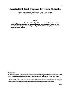
they can be considered as the probabilistic distribution on different kinds of data. The weighted sum of former outputs and current outputs on specific kind of data can be considered as the probability. The outputs of former segmentations are stored. When a new segmentation of sample points occurs, Sensors 2017, 17, 549 13 of 17 the current DNN output is computed and the recognition is drawn considering former outputs. The recognition can be drawn out when every segmentation of sample points is collected. Although the memory is the and timeCWRU delay remains accuracy of increased, DNN on IMS bearing unchanged. data is 94.4% and 94.4%, respectively. The classification As shown inperfect. Tables 2However, and 5, the total accuracy on thesamples IMS bearing can reach theDNN best accuracy is not so if the outputs of former whichdataset is computed by the value by setting the number of hidden layers of the DNN as five and four, respectively. The best are taken into consideration, the classification accuracy on test data will show a significant progress. DNN model is adopted to learn the local characteristics of the time series data of above two datasets. The sigmoid function is used as the activation function so the output of DNN is during 0 and 1 and The be total accuracy as onthe theprobabilistic IMS bearing distribution dataset is 94.4% when the model only takes 7.5 ms of sum data they can considered on different kinds of data. The weighted into account. 7.5 ms is the time length of one segment of data which is used in the IMS experiment. of former outputs and current outputs on specific kind of data can be considered as the probability. When one former segmentation output taken into consideration, the totalof accuracy over The outputs of former segmentations areisstored. When a new segmentation sample jumps points to occurs, 97% as shown in Figure 7a. The classification accuracy of a single kind of data also improves when the current DNN output is computed and the recognition is drawn considering former outputs. the time length is setbe todrawn be longer. The total classification accuracy on the IMS bearing dataset can be The recognition can out when every segmentation of sample points is collected. Although increased to is 100% if the time length is set to be 45 ms, that is to say, five former segments are taken the memory increased, the time delay remains unchanged. into account. As shown in Tables 2 and 5, the total accuracy on the IMS bearing dataset can reach the best value In thethe same way, the accuracy on the CWRU also improves aThe lot with the increase by setting number of hidden layers of the DNNbearing as five dataset and four, respectively. best DNN model ofadopted time length, as shown in Figure 7b. The time length for a single segmentation is 8.33 ms. However, is to learn the local characteristics of the time series data of above two datasets. the outer raceaccuracy faults at on 12 the o’clock 6)dataset are notiseasy to when recognize. The classification of The total IMS (label bearing 94.4% the model only takes 7.5accuracy ms of data outeraccount. race faults data can of reach 98% of when timeislength is set be experiment. longer than into 7.5 at ms12iso’clock the time length oneover segment datathe which used in theto IMS 25 ms and it fluctuates with the increase of the time length. The classification accuracies of sixtokinds When one former segmentation output is taken into consideration, the total accuracy jumps over of data can all get 100% with enough long time length. When the time length is equal to 58.33 the 97% as shown in Figure 7a. The classification accuracy of a single kind of data also improvesms, when totaltime classification accuracy on test data 100%. Figureaccuracy 7a and on Table show the testing the length is set to be longer. The totalisclassification the 8IMS bearing datasetdataset can be accuracies of proposed model considering temporal coherence of IMS bearing dataset. Figure 7b and increased to 100% if the time length is set to be 45 ms, that is to say, five former segments are taken Table 9 show the accuracies of CWRU bearing dataset. into account.
(a)
(b)
Figure 7. Classification accuracies of IMS (a) and CWRU (b) bearing dataset considering different time Figure 7. Classification accuracies of IMS (a) and CWRU (b) bearing dataset considering different time length. The horizontal axis is the time length of data which the model takes into consideration and length. The horizontal axis is the time length of data which the model takes into consideration and the the vertical axis is the accuracy. vertical axis is the accuracy.
In the same way, the accuracy on the CWRU bearing dataset also improves a lot with the increase of time length, as shown in Figure 7b. The time length for a single segmentation is 8.33 ms. However, the outer race faults at 12 o’clock (label 6) are not easy to recognize. The classification accuracy of outer race faults at 12 o’clock data can reach over 98% when the time length is set to be longer than 25 ms and it fluctuates with the increase of the time length. The classification accuracies of six kinds of data can all get 100% with enough long time length. When the time length is equal to 58.33 ms, the total classification accuracy on test data is 100%. Figure 7a and Table 8 show the testing dataset accuracies of proposed model considering temporal coherence of IMS bearing dataset. Figure 7b and Table 9 show the accuracies of CWRU bearing dataset.
Sensors 2017, 17, 549
14 of 17
Table 8. Classification accuracies considering temporal coherence on IMS dataset. Accuracies on Different Labels
Time (ms) 7.5 15 22.5 30 37.5 45
1
2
3
4
Total
98.9% 100% 100% 100% 100% 100%
91.5% 97.1% 98.2% 99.6% 100% 100%
100% 100% 100% 100% 100% 100%
87.1% 93.0% 97.8% 98.5% 98.9% 100%
94.4% 97.5% 99.0% 99.5% 99.7% 100%
Table 9. Classification accuracies considering temporal coherence on CRWU dataset. Accuracies on Different Labels
Time (ms) 8.33 16.67 25 33.33 41.67 50 58.33
1
2
3
4
5
6
Total
100% 100% 100% 100% 100% 100% 100%
88.4% 95.0% 100% 100% 100% 100% 100%
90.9% 95.0% 98.3% 98.3% 100% 99.1% 100%
95.0% 98.3% 98.3% 100% 100% 100% 100%
99.2% 100% 100% 100% 100% 100% 100%
92.6 95.8% 98.3% 100% 99.2% 99.1% 100%
94.4% 97.4% 99.2% 99.7% 99.9% 99.7% 100%
4. Discussion 4.1. The Selection of the DNN Structure The number of neurons in the first layer, i.e., the input layer, is same as the number of data points of one segmentation. The reason is that raw data points collected by the sensors are directly used as DNN inputs. Their dimensionalities must be same. In the IMS bearing dataset, one segment contains 150 data points which is a quarter of the data points collected in one rotation. The sampling rate is 20 kHz and the rotation speed is 2000 RPM so it can be calculated that 600 data points are collected in one rotation. In the CWRU bearing dataset, one segment contains 100 data points which is also approximately a quarter of the data points collected in one rotation. It also can be calculated by the sampling rate 12 kHz and rotation speed 1797 RPM that approximately 401 data points are in one rotation. The number of neurons in the last layer, i.e., the output layer, is the same as the number of data categories, which includes one normal type and several fault types. In the IMS bearing dataset, there are four types of data, including normal data, inner race fault data, outer race fault data and roller defect data, so the number of output neurons is four. In the CWRU bearing dataset, there are six kinds of data, including normal data, inner race fault data, ball defect data, outer race fault at center @ 6:00 data, outer race fault at orthogonal @ 3:00 data, outer race fault @ oppositely @ 12:00 data, therefore, the number of output neurons is set to six. There is no strict criterion for selecting the number of neurons in hidden layers. An upper bound of neurons is set. The classification accuracies will be different when these parameters are set to be different. The number of first hidden layers can be set to be larger or smaller than or equal to the number of input layers. The number of neurons in a former hidden layer is simply set to be larger than the number of neurons in the next layer so as to learn more abstract representations. In this paper, the specific numbers of hidden layers are chosen according to the experimental requirements such as the number of first layer and computational complexity. The number of hidden layers is set to various values and they will give different performance. Comparisons are made for models with different structure. Then the best DNN model is chosen. The experimental results show that the performance of DNN does not always increase with more
Sensors 2017, 17, 549
15 of 17
layers. For example, in the CWRU bearing dataset experiment, the performance of the seven layers model decreased compared with shallower models. Therefore, the DNN structure is selected according to the performance. 4.2. Comparision with Other Methods Table 10 shows classification accuracies of different methods, including Genetic Algorithm with Random Forest [22], Chi Square Features with different classifiers [23], Continuous Wavelet Transform with SVM, Discrete Wavelet Transform with ANN [24], Statistical Locally Linear Embedding with SVM [8] and the method proposed in this paper. Table 10. Classification accuracy of different methods. Methods
Accuracies
Genetic Algorithm + Random Forest 8 Chi Square Features + Random Forest 8 Chi Square Features + SVM 7 Chi Square Features + SVM 8 Chi Square Features + Multilayer Perceptron Continuous Wavelet Transform + SVM Discrete Wavelet Transform (mother wavelet: morlet) + ANN Discrete Wavelet Transform (mother wavelet: daubechies10) + ANN Statistical Locally Linear Embedding + SVM DNN considering temporal coherence
97.81% 93.33% 100% 92% 97.33% 100% 96.67% 93.33% 94.07% 100%
Genetic Algorithm with Random Forest can get an accuracy of 97.81%. Conventional fault diagnosis methods usually select specific features as the classification basis. Some methods can get perfect 100% classification accuracy with the best features. Therefore the features which are extracted from the raw data are the crucial points of these methods. Selecting appropriate features makes a great contribution to the discrimination of the data collected by sensors. For example, chi square feature ranking with SVM can achieve a classification accuracy of 100% when eight features are chosen as the basis. However, the classification accuracy will decrease to 92% when seven features are used. Another example is that the classification accuracy of Discrete Wavelet Transform (Morlet mother wavelet) with ANN can be 96.67%, but it will decrease to 93.33% when the mother wavelet is changed to Daubechies10. Another drawback of these methods is that they do not consider the temporal coherence, i.e., the former data is not taken into account in the current classification process. This paper proposed a DNN-based model without a feature selection process. It learns characteristics directly from raw sensor data and also considers the temporal coherence. The classification accuracy can reach 100%. 5. Conclusions In this paper, a DNN-based model to classify faults is proposed. The raw time series data collected by sensors are directly used as inputs of the proposed model because DNNs are component of learning characteristics from raw sensor data. Conventional fault diagnosis usually focuses on the feature extraction with signal processing methods such as time domain and frequency domain feature representation, EMD, IMF, HHT and DWT. Feature extraction from the time series data is the key point of these approaches, therefore, different data require different feature extraction methods. The proposed model can autonomously learn the features that are helpful to machinery fault diagnosis. Expertise in feature selection and signal processing is not required. Also, the temporal coherence is taken into consideration. This is a great advantage for prognostics using the proposed method when comparing with conventional fault diagnosis approaches which require of signal processing expertise and extract specific time domain or frequency domain features.
Sensors 2017, 17, 549
16 of 17
Acknowledgments: This work received financial support from the National Natural Science Foundation of China (No. 61202027), the Beijing Natural Science Foundation of China (No. 4122015), and the Project of Construction of Innovative Teams and Teacher Career Development for Universities and Colleges under Beijing Municipality (No. IDHT20150507). Acknowledgement is made for the measurements used in this work provided through data-acoustics.com IMS database and CWRU database. Author Contributions: Ran Zhang and Lifeng Wu conceived and designed the experiments; Zhen Peng performed the experiments; Yong Guan analyzed the data; Beibei Yao contributed analysis tools; Ran Zhang wrote the paper. All authors contributed to discussing and revising the manuscript. Conflicts of Interest: The authors declare no conflict of interest.
References 1.
2.
3. 4.
5.
6.
7.
8. 9. 10. 11. 12. 13. 14. 15. 16. 17.
Ciabattoni, L.; Cimini, G.; Ferracuti, F.; Grisostomi, M. Bayes error based feature selection: An electric motors fault detection case study. In Proceedings of the 42nd Annual Conference of IEEE Industrial Electronics Society, Piazza Adua, Florence, Italy, 24–27 October 2016; pp. 003893–003898. Hocine, F.; Ahmed, F. Electric motor bearing diagnosis based on vibration signal analysis and artificial neural networks optimized by the genetic algorithm. In Applied Condition Monitoring; Chaari, F., Zimroz, R., Bartelmus, W., Haddar, M., Eds.; Springer: Berlin/Heidelberg, Germany, 2016; Volume 4, pp. 277–289. Samanta, B.; Al-Balushi, K.R.; Al-Araimi, S.A. Bearing fault detection using artificial neural networks and support vector machines with genetic algorithm. Soft Comput. 2006, 10, 264–271. [CrossRef] Jia, F.; Lei, Y.; Lin, J.; Jing, L.; Xin, Z.; Na, L. Deep neural networks: A promising tool for fault characteristic mining and intelligent diagnosis of rotating machinery with massive data. Mech. Syst. Signal Process. 2015, 72–73, 303–315. [CrossRef] Giantomassi, A.; Ferracuti, F.; Iarlori, S.; Ippoliti, G.; Longhi, S. Signal Based Fault Detection and Diagnosis for Rotating Electrical Machines: Issues and Solutions. In Studies in Fuzziness and Soft Computing; Giantomassi, A., Ferracuti, F., Iarlori, S., Ippoliti, G., Longhi, S., Eds.; Springer: Berlin/Heidelberg, Germany, 2015; Volume 319, pp. 275–309. Ali, J.B.; Fnaiech, N.; Saidi, L.; Chebel-Morello, B.; Fnaiech, F. Application of empirical mode decomposition and artificial neural network for automatic bearing fault diagnosis based on vibration signals. Appl. Acoust. 2015, 89, 16–27. Yu, X.; Ding, E.; Chen, C.; Liu, X.; Li, L. A novel characteristic frequency bands extraction method for automatic bearing fault diagnosis based on hilbert huang transform. Sensors 2015, 15, 27869–27893. [CrossRef] [PubMed] Wang, X.; Zheng, Y.; Zhao, Z.; Wang, J. Bearing fault diagnosis based on statistical locally, linear embedding. Sensors 2015, 15, 16225–16247. [CrossRef] [PubMed] Lou, X.; Loparo, K.A. Bearing fault diagnosis based on wavelet transform and fuzzy inference. Mech. Syst. Signal Process. 2004, 18, 1077–1095. [CrossRef] Malhi, A.; Gao, R.X. PCA-based feature selection scheme for machine defect classification. IEEE Trans. Instrum. Meas. 2005, 53, 1517–1525. [CrossRef] Wu, L.; Yao, B.; Peng, Z.; Guan, Y. Fault Diagnosis of roller bearings based on a wavelet neural network and manifold learning. Appl. Sci. 2017, 7, 158. [CrossRef] Li, C.; Sánchez, R.V.; Zurita, G.; Cerrada, M.; Cabrera, D. Fault diagnosis for rotating machinery using vibration measurement deep statistical feature learning. Sensors 2016, 16, 895. [CrossRef] [PubMed] Mariela, C.; René Vinicio, S.; Diego, C.; Grover, Z.; Chuan, L. Multi-stage feature selection by using genetic algorithms for fault diagnosis in gearboxes based on vibration signal. Sensors 2015, 15, 23903–23926. Hinton, G.E.; Salakhutdinov, R.R. Reducing the dimensionality of data with neural networks. Science 2006, 313, 504–507. [CrossRef] [PubMed] Shah, S.A.A.; Bennamoun, M.; Boussaid, F. Iterative deep learning for image set based face and object recognition. Neurocomputing 2015, 174, 866–874. [CrossRef] Noda, K.; Yamaguchi, Y.; Nakadai, K.; Okuno, H.G.; Ogata, T. Audio-visual speech recognition using deep learning. Appl. Intell. 2015, 42, 722–737. [CrossRef] Zhou, S.; Chen, Q.; Wang, X. Active deep learning method for semi-supervised sentiment classification. Neurocomputing 2013, 120, 536–546. [CrossRef]
Sensors 2017, 17, 549
18. 19. 20.
21. 22. 23.
24.
17 of 17
Hinton, G.E.; Osindero, S.; Teh, Y.W. A Fast Learning algorithm for deep belief nets. Neural Comput. 2006, 18, 1527–1554. [CrossRef] [PubMed] Larochelle, H.; Bengio, Y.; Louradour, J.; Lamblin, P. Exploring strategies for training deep neural networks. J. Mach. Learn. Res. 2009, 10, 1–40. Lee, J.; Qiu, H.; Yu, G.; Lin, J. Rexnord Technical Services, IMS, University of Cincinnati. Bearing Data Set, NASA Ames Prognostics Data Repository. NASA Ames Research Center: Moffett Field, CA, USA. Available online: https://ti.arc.nasa.gov/tech/dash/pcoe/prognostic-data-repository/#bearing (accessed on 14 November 2016). Loparo, K. Bearings Vibration Data Set, Case Western Reserve University. Available online: http://www. eecs.case.edu/laboratory/bearing/welcome_overview.htm (accessed on 20 July 2012). Cerrada, M.; Zurita, G.; Cabrera, D.; Sánchez, R.V.; Artés, M.; Li, C. Fault diagnosis in spur gears based on genetic algorithm and random forest. Mech. Syst. Signal Process. 2016, 70–71, 87–103. [CrossRef] Vinay, V.; Kumar, G.V.; Kumar, K.P. Application of chi square feature ranking technique and random forest classifier for fault classification of bearing faults. In Proceedings of the 22th International Congress on Sound and Vibration, Florence, Italy, 12–16 July 2015. Konar, P.; Chattopadhyay, P. Bearing fault detection of induction motor using wavelet and support vector machines (SVMs). Appl. Soft Comput. 2011, 11, 4203–4211. [CrossRef] © 2017 by the authors. Licensee MDPI, Basel, Switzerland. This article is an open access article distributed under the terms and conditions of the Creative Commons Attribution (CC BY) license (http://creativecommons.org/licenses/by/4.0/).