Hindawi Publishing Corporation Journal of Sensors Volume 2016, Article ID 7436841, 17 pages http://dx.doi.org/10.1155/2016/7436841
Research Article Faulty Line Selection Method for Distribution Network Based on Variable Scale Bistable System Xiaowei Wang,1 Jie Gao,2 Guobing Song,1 Qiming Cheng,2 Xiangxiang Wei,3 and Yanfang Wei4 1
School of Electrical Engineering, Xi’an Jiaotong University, Xi’an, Shaanxi Province 710049, China College of Automation Engineering, Shanghai University of Electric Power, Shanghai, China 3 College of Information and Electrical Engineering, China Agricultural University, Beijing, China 4 School of Electrical Engineering and Automation, Henan Polytechnic University, Jiaozuo 454000, China 2
Correspondence should be addressed to Jie Gao;
[email protected] Received 17 June 2016; Accepted 17 July 2016 Academic Editor: Antonio Fern´andez-Caballero Copyright © 2016 Xiaowei Wang et al. This is an open access article distributed under the Creative Commons Attribution License, which permits unrestricted use, distribution, and reproduction in any medium, provided the original work is properly cited. Since weak fault signals often lead to the misjudgment and other problems for faulty line selection in small current to ground system, this paper proposes a novel faulty line selection method based on variable scale bistable system (VSBS). Firstly, VSBS is adopted to analyze the transient zero-sequence current (TZSC) with different frequency variety scale ratio and noise intensity, and the results show that VSBS can effectively extract the variation trends of initial stage of TZSC. Secondly, TZSC is input to VSBS for calculation with Runge-Kutta equations, and the output signal is chosen as the characteristic currents. Lastly, correlation coefficients of every line characteristic current are used as the index to a novel faulty line selection criterion. A large number of simulation experiments prove that the proposed method can accurately select the faulty line and extract weak fault signals in the environment with strong noise.
1. Introduction As an important part of the power system, distribution network is closely associated with its users and also has direct impact on the users. Data show that 80% of fault occurring in distribution network is single phase-to-ground fault. When single phase-to-ground fault occurs, the line voltage value is still symmetrical, the fault current is weak, and it could run 1 to 2 hours after fault occurs, which significantly improves the reliability of power supply. However, during the single phase-to-ground fault period, nonfault phase voltage could rise, which will threaten the system insulation and result in interphase shortage, protection tripping, power supply outage, and other problems. Because of the weak fault signal and the harsh working condition, faulty line selection becomes difficult. Therefore, it is necessary to carry out further research in this area [1, 2].
At present, scholars have put forward various faulty line selection methods. Based on different characteristic components, faulty line selection methods for single phaseto-ground could be divided into 3 categories, that is, signal injection method [3], steady-state component method [4], and transient component method [5, 6]. The signal injection method needs additional signal device and its engineering realization is complex. In steady-state component method the characteristic signal is weak, which makes the result unreliable, while the transient characteristics method is more reliable and applicable because the transient characteristics component is larger than steady component and it will not be influenced by the arc suppression coil and it will need no additional devices [7–11]. Papers [7, 8] use wavelet transform to extract characteristic information for faulty line selection, but the wavelet transform is easily influenced by noise, and the chosen characteristic frequency band may be nonvalid
2
Journal of Sensors Line l1
Rg
Phase C Phase B Phase A
Cu
Ck
Cn
Line lk ···
Rp Lp
C1
···
u
Line lN
(a) The structure of small current to ground system
i0.t
Rg
L0
Rp
i0C.t
U(t) i0L.t
C0 Lp
(b) TZSC equivalent circuit of single phase ground
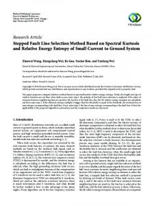
Figure 1: The structure and TZSC equivalent circuit of small current to ground system.
transient faulty component. In addition, different wavelet basis function would lead to different extraction results and thus lead to error judgment. Paper [9] adopts Prony algorithm to fit TZSC signal when fault occurs. This method not only effectively avoids the effect of current transformer saturation flux density on collected signals but also improves the overall Prony fitting precision to a certain extent; but its calculation amount is large, its fitting order is difficult to determine, and the antinoise ability is not strong. In [10], the support vector machine shows its advantages in solving the problem of small sample, nonlinear, and high dimensional pattern recognition, but the recognition ability is easily influenced by its own parameters. Paper [11] uses Empirical Mode Decomposition (EMD) of TZSC to extract the five harmonic components in characteristic components and input them into Duffing oscillator to achieve faulty line selection according to the change of phase diagram. But when TZSC is greatly interfered with, modal aliasing phenomenon of EMD would arise and cause error judgment. Paper [12] employs the ratios of the first half-wave extreme and Spectral Kurtosis relative energy entropy from TZSC to build the stepped faulty line selection method. Paper [13] uses the S-transform to obtain the modulus and phase information of electric components at each frequency point, and this information is employed to detect the faulty line. In [14], Hilbert-Huang transform is used to decompose the TZSC, and then the most high frequency component of the intrinsic mode functions (IMF) can be obtained, and, based on this, the selection criterion is built; however, the decomposition process may cause modal aliasing. Paper [15] adopts evidence uncertainty reasoning and compared abnormal events to reduce computation amount and to improve the accuracy of faulty line selection. Paper [16] employs cross-correlation theory to calculate the integrated correlation coefficient of pure fault component of zero-modulus current for each line and takes the line with the smallest one as the faulty line. Paper [17] carries out the wavelet transform to decompose the transient zero-sequence current for each line, calculates the high and low frequency wavelet energies according to the wavelet coefficients, and selects the faulty line according to the maximum value of high or low frequency energy; however, in the strong noise background, the waveform and energy of weak TZSC will be affected.
In recent years, the research on stochastic resonance has made great progress. Stochastic resonance is a new practical technology which uses stochastic resonance principle to detect weak signal, and its research and application have spread into physical fields [18, 19], signal processing [20, 21], mechanical fault diagnosis [22], biology [23], neural network [24], and other academic fields; however, the research on this technology in power system is still needed. Therefore, with detailed study of the effect of TZSC on bistable system, this paper proposes a novel faulty line selection method for small current to ground system based on stochastic resonance theory. For signal feature extraction, the method employs VSBS to deal with TZSC and, then, choose the initial stage of output signal as characteristic current; for faulty line selection criterion, a novel faulty line selection criterion, which is based on cross-correlation coefficient sign, is proposed through calculating correlation coefficient of characteristic signal.
2. Characteristic Analysis of Single Phase-toGround Fault The structure of small current to ground system is shown in Figure 1(a); when it experiences single phase-to-ground, the TZSC analysis circuit of faulty line is shown in Figure 1(b). In Figure 1, 𝐶0 and 𝐿 0 are zero-sequence capacitance and inductance, respectively, 𝑅𝑔 is transition resistance of ground point, 𝑅𝑝 and 𝐿 𝑝 are, respectively, equivalent resistance and inductance of arc suppression coil, and 𝑈(𝑡) is zero-sequence voltage. When distribution network fault occurs, from Figure 1(b), the TZSC flowing through the fault point 𝑖0,𝑡 is shown as [25] 𝑖0,𝑡 = 𝑖0𝐿,𝑡 + 𝑖0𝐶,𝑡 = 𝐼𝐿𝑚 cos 𝜑𝑒−𝑡/𝜏𝐿 + 𝐼𝐶𝑚 (
𝜔𝑓 𝜔
(1)
sin 𝜑 sin 𝜔𝑡 − cos 𝜑 cos 𝜔𝑓 𝑡) 𝑒−𝛿𝑡 ,
where 𝑖0𝐿,𝑡 and 𝑖0𝐶,𝑡 are inductive current and capacitive current of TZSC, and its initial values are 𝐼𝐿𝑚 and 𝐼𝐶𝑚 , respectively (𝐼𝐶𝑚 = 𝑈𝑝ℎ𝑚 𝜔𝐶, 𝐼𝐿𝑚 = 𝑈𝑝ℎ𝑚 /𝜔𝐿), 𝑈𝑝ℎ𝑚 is phase voltage amplitude, 𝜔 is angular frequency of power frequency,
Journal of Sensors
3
3. Signal-Detecting Ability of Variable Scale Bistable System The bistable system for studying stochastic resonance is shown in [28] 𝑠𝑝 (𝑡) =
𝑑 (−𝑎𝑥2 /2 + 𝑏𝑥4 /4) d𝑥 =− + 𝑠𝑖 (𝑡) + Γ (𝑡) , d𝑡 d𝑥
𝜕2 + 𝐷 2 𝜌 (𝑥, 𝑡) . 𝜕𝑥
D = 0.13 Rout = 0.12
0.15 0.1 0.05 0
0
0.1
0.2
0.3
0.4
0.5
0.6
0.7
0.8
0.9
1
D
Figure 2: The curve of 𝑅out with changed 𝐷.
signal-to-noise ratio of bistable system can be obtained and shown in 2
𝑅out
√2𝜇2 𝐴2 𝑒−𝜇 /4𝐷 = . 4𝐷2
(4)
Supposing 𝜇 is 1 and 𝐴 is 0.2, the curve of 𝑅out is shown in Figure 2 when 𝐷 changed. The feature of Figure 2 is that, with the rise of 𝐷, 𝑅out presents a trend of increasing and begins to decrease when 𝐷 reached 0.13, which is the feature of stochastic resonance. So the bistable system can use noise to increase 𝑅out of signal; that is, the weak signal is amplified and detected. Under the small parameters of adiabatic approximation condition, the theoretical analysis of stochastic resonance of bistable system coincides with the numerical simulation of the bistable system [28]. However, it is improper to apply the method of small parameters stochastic resonance directly to the processing of signals with large parameters. Reference [27] introduces variable scale stochastic resonance to the process and gets better results; however, when the signal is TZSC, what change will happen to stochastic resonance feature of bistable system, and what rules can we get? This section will focus on the influence of each parameter on bistable system and try to figure out the VSBS characteristics under the effect of TZSC.
(2)
where 𝑡 is time, 𝑠𝑖 (𝑡) is input signal, Γ(𝑡) is noise whose intensity is 𝐷, 𝑠𝑝 (𝑡) is output signal, and 𝑥 is the speed of Brownian particle. According to Fokker-Planck equation, the probability distribution function of 𝑥 is shown in (3) when 𝑠𝑖 (𝑡) is 𝐴 sin(2𝜋𝑓0 𝑡) and 𝑎 and 𝑏 are equal to 𝜇 and 1, where 𝐴 and 𝑓0 are the amplitude and frequency of periodic signal: 𝜕𝜌 (𝑥, 𝑡) 𝜕 = − [−𝜇𝑥 − 𝑥3 + 𝐴 sin (2𝜋𝑓0 𝑡) 𝜌 (𝑥, 𝑡)] 𝜕𝑡 𝜕𝑥
0.2
Rout
𝜔𝑓 and 𝛿 are oscillation angular frequency and attenuation coefficient of TZSC, 𝜏𝐿 is decay time constant of inductive current, and 𝜑 is initial phase angel. From (1), when single phase-to-ground fault occurs in distribution network, the transient capacitance current has the characteristic of periodic attenuation oscillation. And [1] indicates that the free oscillation frequency of overhead line is within 300 Hz to 1500 Hz and the free oscillation frequency of cable lines is 1500 Hz∼3000 Hz. In addition, studies show that when single phase-toground fault occurs, the traveling wave pole is consistent with the overall changing trend of initial stage TZSC in transient process, so the mutation direction characteristic of initial stage TZSC can be used to replace the traveling wave polarity characteristic of TZSC, which can greatly reduce the hardware requirements and improve the reliability of faulty line selection [26]. Besides, whether it is big initial fault angle or small initial fault angle, the whole changing trend of faulty line is opposite to that of nonfaulty line in TZSC initial stage. But the introduction of arc suppression coil will greatly reduce ground fault current of distribution network, and when the fault occurs in voltage zero position, the changing trend of the initial stage TZSC is not easy to distinguish, which will make faulty line selection more difficult. Hence, in some faulty conditions, it can be seen from the above analysis that TZSC of distribution network belongs to weak signal. As stochastic resonance (SR) theory has the unique advantage of amplification and detection of weak signals [27], it is helpful to employ the stochastic resonance theory to detect TZSC which is used to select the faulty line.
(3)
Since (3) has nonautonomous −(𝜕/𝜕𝑥)[𝐴 sin(2𝜋𝑓0 𝑡)𝜌(𝑥, 𝑡)], it has no steady-state solution; that is, it can not have exact expression. However, in the adiabatic approximation condition with 𝐴 ≪ 1, 𝐷 ≪ 1, and 𝑓0 ≪ 1, the output
3.1. Variable Metric Algorithm and Its Evaluation Index. The principle of variable metric algorithm is to transform high frequency into low frequency in order to make the large parameter signal close to or meeting small parameters conditions of stochastic resonance, which means that the frequency is compressed and then detected by bistable system. The Calculation Process of Variable Scale. According to the frequency and sampling frequency of signals, a frequency compression-scale ratio (CR) is determined, based on which the compression sampling frequency 𝑓𝑠𝑟 is defined (𝑓𝑠𝑟 = 𝑓𝑠 /CR). Then numerical calculation step ℎ (ℎ = 1/𝑓𝑠𝑟 ) is obtained from 𝑓𝑠𝑟 , and, finally, the response output of bistable system is numerically calculated. Since TZSC are generally broadband signals and their frequency range is not confined to one or a small number of frequencies but distributed in a wide frequency band, to which the traditional signal-to-noise ratio measurement cannot be effectively applied, it is necessary to develop other measurement indexes.
Journal of Sensors 100
20
50
10 i (A)
i (A)
4
0
−10
−50 −100
0
0
0.05
0.1
0.15
0.2
0.25 t (s)
0.3
0.35
0.4
0.45
−20
0.5
0
0.05
4
0.4
2
0.2
0.2
0.25 t (s)
0.3
0.35
0.4
0.45
0.5
0 −2
0 −0.2
0.15
(b) Input signal without noise
0.6 i (A)
i (A)
(a) Input signal with noise
0.1
0
0.05
0.1
0.15
0.2
0.25 t (s)
0.3
0.35
0.4
0.45
0.5
−4
0
0.05
0.1
(c) Output signal 1
0.15
0.2
0.25 t (s)
0.3
0.35
0.4
0.45
0.5
(d) Output signal 2
Figure 3: The simulation for bistable system.
Reference [27] shows that although nonlinear Langevin equation cannot accurately predict the motion of Brownian particles, it can well predict the statistical properties of the particle orbits. So, this paper uses cross-correlation coefficient as a measure to describe the response of VSBS whose input signal is weak aperiodic signal. The covariance Cov(𝑠𝑝 (𝑡), 𝑠𝑖 (𝑡)) and cross-correlation coefficients 𝜌𝑝𝑖 of two signals are shown in Cov (𝑠𝑝 (𝑡) , 𝑠𝑖 (𝑡)) = 𝐸(𝑠𝑝 ⋅𝑠𝑖 ) − 𝐸𝑠𝑝 𝐸𝑠𝑖 𝜌𝑝𝑖 =
Cov (𝑠𝑝 (𝑡) , 𝑠𝑖 (𝑡)) √𝐷 (𝑠𝑝 (𝑡))√𝐷 (𝑠𝑖 (𝑡))
.
(5)
Additionally, in the initial faulty stage, the overall changing trend of TZSC of faulty line is opposite to that of nonfaulty line, so this paper focuses on the changing trend of input signal and output signal. 3.2. Simulation of Variable Scale Bistable System 3.2.1. Simulation of Nonintroducing Variable Scale. Supposing there is a set of measured signals, the sampling points are 500, the corresponding parameters of (2) are 𝑎 = 𝑏 = 1, 𝐴 = 20 A, 𝑓0 = 40 Hz, and 𝐷 = 100 db, respectively, and the value of sampling frequency 𝑓𝑠 is 1000 Hz. Fourth-order Runge-Kutta algorithm is adopted to calculate (2). And the value of crosscorrelation coefficients 𝜌𝑝𝑖 of 𝑠𝑖 (𝑡) and 𝑠𝑝 (𝑡) is −0.0078, whose results are shown in Figure 3. Figure 3(a) shows the result of 𝑠𝑖 (𝑡) with noise intensity as 100 db, Figure 3(b) shows 𝑠𝑖 (𝑡) without noise, and Figure 3(c) shows 𝑠𝑝1 (𝑡) without being solved by variable scale. It can be known from Figure 3 and 𝜌𝑝𝑖 that when both weak signal frequencies 𝑓0 and 𝐷 are large parameters (larger than 1), the output and input of the system differ dramatically, and the information contained in the output signal will not
be able to represent the original signal. That is why the stochastic resonance method with small parameters can not be directly applied to large parameters signal, so the detection is ineffective. 3.2.2. Simulation of Introducing Variable Scale. Bring in variable scale thought, choose CR as 100, 𝑎 = 𝑏 = 1, 𝐴 = 20 A, 𝑓0 = 40 Hz, 𝐷 = 100 db, and the value of sampling frequency 𝑓𝑠 is 1000 Hz; calculate (2) with fourth-order Runge-Kutta algorithm and cross-correlation coefficients 𝜌𝑝𝑖 of 𝑠𝑖 (𝑡) and 𝑠𝑝 (𝑡), 𝜌𝑝2 𝑖 will be obtained, and its value is 0.8088. The result is shown in Figure 3(d). Figure 3(d) shows that after the treatment of VSBS, the waveform of output signal 𝑠𝑝 (𝑡) becomes orderly. Compared to Figure 3(c), the cross-correlation coefficients between 𝑠𝑖 (𝑡) and 𝑠𝑝 (𝑡) have obviously improved as well as the amplitude value of 𝑠𝑝 (𝑡); besides, 𝑠𝑝 (𝑡) and 𝑠𝑖 (𝑡) belong to strong correlation. Therefore, through frequency conversion, the disorganized large parameter signal is made clear and orderly; besides, 𝜌𝑝𝑖 is equal to 0.8088, which indicates that 𝑠𝑝 (𝑡) could better represent changing trend of 𝑠𝑖 (𝑡) submerged in noise, achieving the large parameter stochastic resonance or, exactly speaking, a kind of stochastic resonance. 3.3. Transient Zero-Sequence Current Detection. In order to test whether VSBS can detect the TZSC, the ideal TZSC 𝑖𝑧 (𝑡) [29] is defined as below: 𝑖𝑧 (𝑡) = 𝑥1 (𝑡) + 𝑥2 (𝑡) + 𝑥3 (𝑡) + 𝑥4 (𝑡) + Γ (𝑡) ,
(6)
𝑥1 (𝑡) = 5.6 cos (2𝜋 × 50𝑡 + 60∘ ) ,
(7)
𝑥2 (𝑡) = 40𝑒−56𝑡 cos (2𝜋 × 250𝑡 + 30∘ ) ,
(8)
𝑥3 (𝑡) = 72𝑒−102𝑡 cos (2𝜋 × 315𝑡) ,
(9)
𝑥4 (𝑡) = 10𝑒−5.5𝑡 .
(10)
5 200
10
100
100
5
0 −100
0
i (A)
(a) TZSC with noise
150 100 50 0 −50 Initial stage −100 0 0.01
0 −100
0.002 0.004 0.006 0.008 0.01 t (s)
i (A)
200 i (A)
i (A)
Journal of Sensors
0
0 −5
0.002 0.004 0.006 0.008 0.01 t (s) (b) TZSC without noise
0
0.002 0.004 0.006 0.008 0.01 t (s) (c) Characteristic current
Whole stage
Other stages 0.02
0.03
0.04
0.05
0.06
0.07
0.08
t (s) (d) TZSC without noise
Figure 4: Characteristic extraction of TZSC by VSBS.
It can be seen that 𝑖𝑧 (𝑡), which consists of 5 signals, has the characteristic of multifrequency and attenuation; therefore it is a nonperiodic signal. Input it into (2), and its corresponding parameters are 𝑎 = 𝑏 = 1 and 𝐷 = 50 db and sampling frequency is 𝑓𝑠 =100000 Hz. CR is equal to 1000, and then the results of its numerical simulation are shown in Figure 4. Definition of Characteristic Current 𝑖𝑐 (𝑡). Characteristic current is the output signal obtained by solving VSBS with TZSC by fourth-order Runge-Kutta algorithm. Choose nonnoises 𝑖𝑧 (𝑡) and 𝑖𝑐 (𝑡) to calculate cross-correlation coefficient 𝜌𝑐𝑧 , and the value is 0.7628. When only the first 0.01 s of 𝑖𝑧 (𝑡) and 𝑖𝑐 (𝑡) is chosen, as shown in Figure 4(a), the noise causes strong disturbance in the initial stage of 𝑖𝑧 (𝑡), which makes the changing trend not so clear as the original signal. It is known from Figure 4(c) that, after VSBS treatment, the changing trend of 𝑖𝑐 (𝑡) is similar to that of 𝑖𝑧 (𝑡); then, their 𝜌𝑐𝑧 is calculated, and the value has improved to 0.8909. Therefore, VSBS can effectively extract TZSC changing trend of the initial stage. This method can be used to better extract the change trend of TZSC in the initial stage. This paper defines 0∼0.01 s as the initial stage of TZSC, 0.01 s∼∞ as noninitial stage, and signal length as the whole stage. To put it vividly, TZSC from (6) is chosen as the label, and the results are shown in Figure 4(d). 3.4. The Detection Adaptability of TZSC. In order to test detection adaptability of VSBS for TZSC, the paper will analyze frequency compression-scale ratio, noise intensity, the initial value, and signal amplitude, respectively. 3.4.1. Frequency Compression-Scale Ratio (CR). Set 𝑎 = 𝑏 = 1 and 𝐷 = 50 db and sampling frequency 𝑓𝑠 equals 100000 Hz; set CR as 10, 100, 1000, and 5000, respectively, and the change of 𝜌𝑐𝑧 is shown in Table 1. It can be seen from Table 1 that, with the increase of CR, 𝜌𝑐𝑧 between 𝑖𝑧 (𝑡) and 𝑖𝑐 (𝑡) first increases and then decreases;
Table 1: 𝜌cz in different conditions. Condition CR = 10 CR = 100 CR = 1000 CR = 5000 𝐷=0 𝐷 = 50 𝐷 = 100 𝐷 = 1000 𝐷 = 5000 IV = 34.8 IV = 0 IV = −34.8 𝜏 = 1/100 𝜏 = 1/10 𝜏=1 𝜏 = 10 𝜏 = 100
Whole stage 𝜌cz −0.2220 0.4716 0.7628 0.6784 0.7638 0.7628 0.7518 0.6470 0.4286 0.7628 0.8806 0.8555 0.4807 0.7403 0.9221 0.7146 0.7150
Initial stage 𝜌cz −0.3395 0.5300 0.8909 0.7944 0.8874 0.8909 0.8876 0.8641 0.7910 0.8909 0.9221 0.8914 −0.0234 0.1820 0.7130 0.9916 0.9922
the reason is that the increase of CR can gradually compress the frequency band range of 𝑖𝑧 (𝑡) into VSBS’s detection range, and there may be a most suitable CR making the input and output most relevant, but when CR continues to increase, excessive frequency compression will also lead to decrease of gap between different frequencies of 𝑖𝑧 (𝑡), showing the reduction of frequency species, which will further weaken the detection ability of VSBS. In addition, the calculation of cross-correlation coefficients of 𝑖𝑧 (𝑡) and 𝑖𝑐 (𝑡) in initial stage shows that 𝜌𝑐𝑧 has greatly improved, and the changing trend of 𝑖𝑐 (𝑡) is the same as that of 𝑖𝑧 (𝑡), which verifies that VSBS can effectively extract the changing trend of TZSC in initial stage.
Journal of Sensors 5
Amplitude (A)
Amplitude (A)
6
0 −5
0
0.01
0.02
0.03
0.04
0.05
0.06
0.07
0.08
10 5 0 −5
0
0.01
0.02
0.03
t (s)
0 −5
0
0.01
0.02
0.03
0.04 t (s)
0.05
0.06
0.07
0.08
0.05
0.06
0.07
0.08
(b) 𝐷 = 100
5
Amplitude (A)
Amplitude (A)
(a) 𝐷 = 0
0.04 t (s)
0.05
0.06
0.07
0.08
(c) Initial value = 0
10 5 0 −5
0
0.01
0.02
0.03
0.04 t (s)
(d) Initial value = 34.8
Figure 5: Characteristic current under the different conditions.
3.4.2. Noise Intensity (D). Set 𝑎 = 𝑏 = 1, sampling frequency 𝑓𝑠 = 100000 Hz, and CR = 1000. Set noise intensity 𝐷 as 0 db, 50 db, 100 db, 1000 db, and 5000 db, respectively, and the change of cross-correlation coefficient 𝜌𝑐𝑧 is shown in Table 1. The change of characteristic current 𝑖𝑐 (𝑡) is shown in Figure 5(a) when the noise intensity of 𝑖𝑧 (𝑡) is 0 db, and the change of characteristic current 𝑖𝑐 (𝑡) is shown in Figure 5(b) when the noise intensity of 𝑖𝑧 (𝑡) is 100 db. It can be seen from waveform in Figure 5 that the amplitude of 𝑖𝑐 (𝑡) increases with the increase of D, which means that part of the noise energy is transferred to 𝑖𝑐 (𝑡) [27]. In addition, the increases of 𝐷 made the latter part waveform disorderly; however, the changing trend of the waveform in initial stage is clear which shows no difference with the changing trend of nonnoise; therefore, this once again shows that the VSBS can extract initial stage TZSC. From 𝜌𝑐𝑧 in Table 1 we know that, within a certain range of noise intensity, the increase of 𝐷 shows little effect on 𝜌𝑐𝑧 of whole stage and of initial stage, which indicates that VSBS can well extract changing trend of TZSC in initial stage with the disturbance of strong noise. However, excessive noise intensity will produce a wide range of interference frequency components, which will affect the existence of the original signal, resulting in the decrease of cross-correlation coefficient and fuzziness of the changing trend in initial stage. It is worth noting that when the noise intensity is 0, the VSBS can also predict the changing trend of TZSC. 3.4.3. Signal Initial Value (IV). Set 𝑎 = 𝑏 = 1, 𝑓𝑠 = 100000 Hz, CR = 1000, and 𝐷 = 50 db; set initial value of 𝑖𝑧 (𝑡) as 0 and 34.8, respectively, where 34.8 is initial value (IV) of 𝑖𝑧 (𝑡). Then carry out numerical simulation and the change of characteristic current 𝑖𝑐 (𝑡) and cross-correlation coefficient 𝜌𝑐𝑧 is shown in Table 1 and Figure 5. Figure 5(c) is characteristic current 𝑖𝑐 (𝑡) when initial value of 𝑖𝑧 (𝑡) is 0, and Figure 5(d) is characteristic current 𝑖𝑐 (𝑡) when initial value of 𝑖𝑧 (𝑡) is 34.8.
It can be known from Figures 5(c) and 5(d) and Table 1 that when initial value of 𝑖𝑧 (𝑡) is 0, the change trend of 𝑖𝑐 (𝑡) is closest to that of 𝑖𝑧 (𝑡), especially in the initial stage. Either increase or decrease of the initial value will decrease 𝜌𝑐𝑧 , because when initial value of VSBS is 0, any tiny disturbance is likely to cause it to move in the double potential well with large amplitude, so it can better reflect the moving trend of signals. However, when the initial value is too large, tiny disturbance may not be enough to cause a large amplitude motion in the double well potential or only small range of motion in a single potential well, therefore, it will weaken the detection ability of VSBS, and this is consistent with the decrease of 𝜌𝑐𝑧 in Table 1. Another reason for adopting TZSC to select faulty line in this paper is that when the initial value of TZSC is 0, VSBS and faulty line selection can be better combined [30]. 3.4.4. Signal Amplitude. Set 𝑎 = 𝑏 = 1, 𝑓𝑠 = 100000 Hz, CR = 1000, and 𝐷 = 50 db; set the initial value as 0, increase the amplitude of 𝑖𝑧 (𝑡), and set the amplitude factor 𝜏 as 1/100, 1/10, 1, 10, and 100, respectively. It is known from Table 1 that, with the increase of amplitude 𝑖𝑧 (𝑡), cross-correlation coefficient 𝜌𝑐𝑧 of whole stage and initial stage first increases and then decreases, but 𝜌𝑐𝑧 of noninitial stage increases. The reason is that 𝑖𝑧 (𝑡) belongs to damped oscillation signal, and, compared with that of noninitial stage, the amplitude values of initial stage are always larger, and the detection ability of VSBS on 𝑖𝑧 (𝑡) in noninitial stage is weaker. Therefore, appropriate increase of signal value would improve detection ability of VSBS. Based on the above analysis, the features of BSVS detecting TZSC are summarized as follows: (1) Appropriate frequency compression ratio can improve the signal detection performance. (2) For small amplitude signal, appropriate increase of amplitude can improve signal detection performance.
Journal of Sensors (3) For the signal with zero initial value, VSBS has a better detection performance of changing trend in its initial stage. (4) The cross-correlation coefficient of whole stage is always smaller than that of initial stage.
4. Faulty Line Selection Method 4.1. Parameter Setting. Based on the above analysis, this paper will select faulty line according to the following characteristics of VSBS detecting TZSC: A The overall changing trend of TZSC in initial stage between faulty line and nonfaulty line is opposite. B VSBS has excellent detection ability for the changing trend of TZSC in initial stage. C When single phase-to-ground fault occurs in small current to ground system, the free oscillation frequency of overhead lines is generally 300 Hz∼1500 Hz, while the free oscillation frequency of cable lines is 1500 Hz∼3000 Hz. In addition, different fault conditions may cause the TZSC spectrum to transfer into low frequency band [25]. D Appropriate increase of signal amplitude helps to improve detection performance of VSBS. According to A and B, this paper will focus on crosscorrelation coefficient of different lines. Since the TZSC before failure is 0, when calculating cross-correlation coefficients, we will choose T/4 cycle after fault as the initial stage (0.02 s∼0.025 s) in the paper; with C frequency varieties are compressed as much as possible to make frequency varieties into the frequency range which VSBS can detect, in order to enhance the adaptability of the method; therefore, the frequency compression-scale ratio (CR) is set as 1500. Based on D and simulation experiment, when the maximum amplitude of signal is less than 5, we first expand the amplitude by 10 times and then input it into VSBS. In addition, we find that TZSC amplitude before fault is not 0 but a very small value, which needs to be set to 0 before fault. 4.2. Pretreatment of Faulty Line Selection. Take line 𝑙1 as an example: A Choose TZSC of line number 1 from one cycle before fault to one cycle after fault as TZSC 𝑖𝑧 (𝑡), and set the signal one cycle before fault as 0. B Judge whether the maximum amplitude of 𝑖𝑧 (𝑡) is smaller than 5, if it is, carry out C, and if it is not, carry out D. C Expand amplitude of 𝑖𝑧 (𝑡) by 10 times and input it into VSBS to calculate characteristic current 𝑖𝑐 (𝑡). D Directly input 𝑖𝑧 (𝑡) into VSBS to calculate characteristic current 𝑖𝑐 (𝑡). Calculate 𝑖𝑐 (𝑡) of all lines according to the above steps.
7 4.3. Steps of Faulty Line Selection. Take 𝑙𝑗 as an example to explain the steps of faulty line selection. Step 1. Calculate cross-correlation coefficients 𝜌𝑗𝑞 between line number 𝑙𝑗 (𝑗 = 1, 2, 3, . . .) and other lines 𝑙𝑞 (𝑞 = 1, 2, 3, . . . 𝑞 ≠ 𝑗) in initial stage. Step 2. Count positive and negative signs of calculated 𝜌𝑗𝑞 : (1) If all the signs of 𝜌𝑗𝑞 are the same, the output is “−1” and line 𝑙𝑗 is judged as faulty line. (2) If all the signs of 𝜌𝑗𝑞 are not the same, the output is “1” and line 𝑙𝑗 is judged as nonfaulty line. The remaining lines are also judged with the same steps.
5. Case Study 5.1. Simulation Model. ATP-EMTP is used in this paper to simulate the single phase-to-ground fault. The simulation model is shown in Figure 6 and the parameters of simulation model are the same as [31]. 5.2. Simulation Results with Changing Phase and Resistance. Build the simulation model according to the parameters, make fault of line 𝑙1 occur at the point 5 km from the bus, and change the initial fault angle (0∘ , 30∘ , 60∘ , and 90∘ ) and ground resistance for simulation. It is known from [25] that when single phase-to-ground fault of the small current to ground system occurs, the fault resistance value is generally 0 kΩ to 2 kΩ; therefore, the maximum fault resistance is set as 2 kΩ in the paper. Then, select the faulty line according to the proposed method, and the parameters of VSBS are as follows: 𝑎 = 𝑏 = 1 and CR = 1500. In addition, we use (𝑙1 , 0∘ , and 300 Ω) to indicate the fault occurrence in line number 1 when its initial angle is 0∘ and faulty resistance is 300 Ω. The results of their specific cross-correlation coefficients are shown in Table 2 in which 𝜌12 represents cross-correlation coefficient of characteristic currents 𝑙1 and 𝑙2 . The paper takes (𝑙1 , 90∘ , and 2000 Ω) as an example to explicitly show the consequence of VSBS. Under this fault condition, the TZSC of 𝑙2 and 𝑖𝑐 (𝑡) of 𝑙2 are shown in Figures 7(a) and 7(b); the cross-correlation coefficients are shown in Table 3. The comparison of Figures 7(a) and 7(b) shows that, after the treatment of VSBS, the changing speed of 𝑖𝑐 (𝑡) in initial stage becomes slow, and oscillation part is reduced, which makes the changing trend of 𝑖𝑐 (𝑡) in initial stage easier to identify than that of TZSC in initial stage. It can be seen from Figure 7(b) that 𝑖𝑐 (𝑡) waveform of faulty line is steadier than that of nonfaulty lines, because frequency compression makes the part in low frequency band and with strong intensity easy to detect by VSBS, and the part in high frequency band and with weak intensity may be ignored, besides, the intensity of low frequency band fault transient component in the faulty line is much larger than that of nonfaulty line, and, therefore, the characteristic current waveform of faulty line is steadier than that of nonfaulty line. Besides, through simulation, we discover that because the transient
8
Journal of Sensors Overhead line l1 Voltage probe Overhead line Source
Transformer +u + I p s
V
V
I
Overhead line V
I Line Z-T
Line Z-T
Load
I RLC
Grounding resistance +u − I I
Arc suppression coil
Switch
I − u+
Overhead line l2 Overhead line
Overhead line
Line Z-T
Line Z-T
I RLC
Hybrid line l3 Cable line
Overhead line
Line Z-T
Line Z-T
I RLC
Cable line l4 Cable line
Cable line
Line Z-T
Line Z-T
I RLC
Current probe
Figure 6: ATP simulation model.
free oscillation components and zero-sequence steady-state components are offset, the increase of fault resistance also makes waveform 𝑖𝑐 (𝑡) of each line steadier. It can be seen from Table 3 that 𝜌1𝑞 of 𝑙1 and other lines are equal to −0.9732, −0.8092, and −0.7535, respectively; since all of them are the same sign, the output is “−1”; 𝜌2𝑞 of 𝑙2 and other lines are equal to −0.9732, 0.7408, and 0.6597, respectively; since all of them are not the same sign, the output is “1”; therefore, we judged 𝑙1 as faulty line, and the judging result is consistent with simulation.
In summary, we know from Table 2 that TZSC of various fault conditions is, respectively, input into VSBS, and the output judging results are consistent with actual fault situations. Therefore, the proposed method can accurately achieve faulty line selection under different fault resistance and initial fault angle. 5.3. Simulation Results of Fault with Random Gauss White Noise Added. Since signals collected in actual system with fault often carry noise with them, to verify the antinoise
Journal of Sensors
9 Table 2: Results of different initial angle and ground resistance.
Faulty line
Fault situation
𝑙1
(0∘ , 10 Ω) (0∘ , 100 Ω) (0∘ , 500 Ω) (0∘ , 1000 Ω) (0∘ , 1500 Ω) (0∘ , 2000 Ω) (30∘ , 10 Ω) (30∘ , 100 Ω) (30∘ , 500 Ω) (30∘ , 1000 Ω) (30∘ , 1500 Ω) (30∘ , 2000 Ω) (60∘ , 10 Ω) (60∘ , 100 Ω) (60∘ , 500 Ω) (60∘ , 1000 Ω) (60∘ , 1500 Ω) (60∘ , 2000 Ω) (90∘ , 10 Ω) (90∘ , 100 Ω) (90∘ , 500 Ω) (90∘ , 1000 Ω) (90∘ , 1500 Ω) (90∘ , 2000 Ω)
𝜌12
𝜌13
𝜌14
𝜌23
𝜌24
𝜌34
Judgment result
−0.4942 −0.6776 −0.5710 −0.5991 −0.6845 −0.6928 −0.5835 −0.7767 −0.7987 −0.7353 −0.6972 −0.7340 −0.6113 −0.8523 −0.9027 −0.8862 −0.9137 −0.8855 −0.9293 −0.9464 −0.9714 −0.9846 −0.9812 −0.9732
−0.8054 −0.7360 −0.7146 −0.3511 −0.2796 −0.5382 −0.8295 −0.8968 −0.8858 −0.6373 −0.5462 −0.4746 −0.8418 −0.9398 −0.9822 −0.7425 −0.7322 −0.9129 −0.8728 −0.9790 −0.8578 −0.8524 −0.8457 −0.8092
−0.9092 −0.7528 −0.6549 −0.7291 −0.3330 −0.5511 −0.9360 −0.8948 −0.8773 −0.7927 −0.5819 −0.4987 −0.9606 −0.9703 −0.9407 −0.9420 −0.7302 −0.8872 −0.9691 −0.9820 −0.9932 −0.8428 −0.7970 −0.7535
0.7852 0.8573 0.8999 0.7810 0.7057 0.6465 0.8132 0.8668 0.8746 0.8598 0.8233 0.8116 0.8201 0.9080 0.9268 0.8639 0.8450 0.8027 0.9117 0.9549 0.8990 0.8467 0.8033 0.7408
0.6078 0.7034 0.8369 0.7424 0.5993 0.5293 0.6362 0.7265 0.8609 0.9000 0.7478 0.7052 0.6109 0.7461 0.9015 0.9368 0.7847 0.7284 0.8795 0.8879 0.9487 0.7932 0.7265 0.6597
0.7973 0.8744 0.9032 0.6944 0.8385 0.8454 0.7710 0.8485 0.9254 0.7555 0.8720 0.8649 0.7682 0.8808 0.9374 0.7823 0.8721 0.8894 0.7960 0.9346 0.8150 0.8995 0.9038 0.9216
𝑙1 fault 𝑙1 fault 𝑙1 fault 𝑙1 fault 𝑙1 fault 𝑙1 fault 𝑙1 fault 𝑙1 fault 𝑙1 fault 𝑙1 fault 𝑙1 fault 𝑙1 fault 𝑙1 fault 𝑙1 fault 𝑙1 fault 𝑙1 fault 𝑙1 fault 𝑙1 fault 𝑙1 fault 𝑙1 fault 𝑙1 fault 𝑙1 fault 𝑙1 fault 𝑙1 fault
Table 3: Cross-correlation coefficient with (𝑙1 , 90∘ , and 2000 Ω) fault situation. Faulty line 𝑙1
𝜌12
𝜌13
𝜌14
𝜌23
𝜌24
𝜌34
−0.9732 −0.8092 −0.7535 0.7408 0.6597 0.9216
Result 𝑙1
performance of the method, we added 0.5 db or −0.5 db noise intensity to TZSC when fault in different line occurred and set signal before fault as 0. The selection results and specific cross-correlation coefficients are shown in Tables 4 and 5, respectively. Signal-to-noise ratio equaling −0.5 db and fault situations as (𝑙2 , 60∘ , 1500 Ω) are taken as an illustration. The TZSC with noise of 𝑙2 and 𝑖𝑐 (𝑡) of 𝑙2 are shown in Figures 7(c) and 7(d), and the cross-correlation coefficients are shown in Table 6. Firstly, from the faulty line selection method and Table 6, cross-correlation coefficients 𝜌2𝑞 of 𝑙2 and other lines are all negative, so the output is “−1” and 𝜌𝑗𝑞 of other lines are different, so the output is “1”; therefore, we judge line 𝑙2 as faulty line, which is consistent with actual fault situation. Then, comparison of Figures 7(c) and 7(d) shows that, with the disturbance of strong noise, even if the TZSC of each line is submerged in strong noise, the proposed method is still able to effectively extract the changing trend of TZSC in initial stage and can accurately judge the faulty line. Finally,
Tables 4 and 5 indicate that, with the disturbance of different noise intensity, the changing trends of characteristic currents in initial stage between faulty line and nonfaulty line still have a better discrimination after the treatment of VSBS, so we can say the method shows a good antinoise performance. The definition of signal-to-noise ratio [28] shows that the smaller the ratio is, the larger the noise intensity will be; therefore, antinoise performance of the method in this paper is much better than the one proposed in [8], which added 15 db and 0.5 db noise. 5.4. Adaptation Analysis of Faulty Line Selection Method 5.4.1. Different Faulty Lines. When fault occurs in 𝑙2 , 𝑙3 , and 𝑙4 , respectively, we carry out faulty line selection method proposed in the paper to verify its adaptability, and the results and specific cross-correlation coefficients are shown in Table 7. We know from [25] that, with the introduction of cable lines, although the attenuation process of fault transient current becomes shorter, the frequency spectrum principal component of transient component will move to low frequency band, which helps to detect VSBS. Therefore, different line fault conditions will not affect selection results of the method, and excellent results can also be obtained with different fault resistance.
Journal of Sensors 0.4
2
0.2
1 i (A)
i (A)
10
0
−1
−0.2 −0.4
0
0
0.005
0.01
0.015
0.02 t (s)
0.025
0.03
0.035
−2
0.04
0
0.005
10
2
5
1
0
0.02 t (s)
0.025
0.03
0.035
0.04
0.035
0.04
0 −1
−5 −10
0.015
(b) 𝑖𝑐 (𝑡) of 𝑙2 in the (𝑙1 , 90∘ , 2000 Ω)
i (A)
i (A)
(a) TZSC of 𝑙2 in the (𝑙1 , 90∘ , 2000 Ω)
0.01
0
0.005
0.01
0.015
0.02 t (s)
0.025
0.03
0.035
−2
0.04
(c) TZSC of 𝑙2 in the (𝑙2 , 60∘ , 1500 Ω)
0
0.005
0.01
0.015
0.02 t (s)
0.025
0.03
(d) 𝑖𝑐 (𝑡) of 𝑙2 in the (𝑙2 , 60∘ , 1500 Ω)
Figure 7: The TZSC and characteristic current of 𝑙2 for different fault condition.
Table 4: Adding 0.5 db Gauss white noise. Faulty line
Fault situation (0∘ , 300 Ω) (90∘ , 1300 Ω) (30∘ , 400 Ω) (60∘ , 1500 Ω) (60∘ , 200 Ω) (90∘ , 2000 Ω) (0∘ , 600 Ω) (30∘ , 1700 Ω)
𝑙1 𝑙2 𝑙3 𝑙4
𝜌12 −0.5426 −0.7183 −0.7562 −0.5732 0.6424 0.4531 0.1898 0.8354
𝜌13 −0.7043 −0.8165 0.8406 0.5756 −0.7439 −0.1279 0.2342 0.8258
𝜌14 −0.7148 −0.9733 0.8673 0.5700 0.7361 0.1332 −0.1300 −0.1221
𝜌23 −0.4045 0.5301 −0.8435 −0.9466 −0.7997 −0.4213 0.8282 0.8843
𝜌24 0.3447 0.6960 −0.8573 −0.9019 0.5996 0.4255 −0.0314 −0.1130
𝜌34 0.9060 0.7200 0.9282 0.8969 −0.8890 −0.9950 −0.3755 −0.0464
Judgment result 𝑙1 fault 𝑙1 fault 𝑙2 fault 𝑙2 fault 𝑙3 fault 𝑙3 fault 𝑙4 fault 𝑙4 fault
𝜌24 0.7142 0.4627 −0.8542 −0.8958 0.6574 0.4422 −0.0483 −0.5253
𝜌34 0.9197 0.8320 0.9247 0.8216 −0.8804 −0.9832 −0.4239 −0.7236
Judgment result 𝑙1 fault 𝑙1 fault 𝑙2 fault 𝑙2 fault 𝑙3 fault 𝑙3 fault 𝑙4 fault 𝑙4 fault
Table 5: Adding −0.5 db Gauss white noise. Faulty line
Fault situation (0∘ , 300 Ω) (90∘ , 1300 Ω) (30∘ , 400 Ω) (60∘ , 1500 Ω) (60∘ , 200 Ω) (90∘ , 2000 Ω) (0∘ , 600 Ω) (30∘ , 1700 Ω)
𝑙1 𝑙2 𝑙3 𝑙4
𝜌12 −0.5919 −0.4888 −0.7433 −0.6892 0.5730 0.3280 0.6865 0.3201
𝜌13 −0.6906 −0.8292 0.8314 0.5295 −0.4954 −0.5827 0.7746 0.6745
𝜌14 −0.6985 −0.9956 0.8227 0.7051 0.3834 0.6395 −0.2193 −0.3900
Table 6: Cross-correlation coefficients with (𝑙2 , 60∘ , and 1500 Ω) fault situation. Faulty line 𝑙2
𝜌12
𝜌13
𝜌14
𝜌23
𝜌24
𝜌34
−0.6892 0.5295 0.7051 −0.8987 −0.8958 0.8216
Result 𝑙2
5.4.2. Different Fault Distance. Since the distance of fault point is different in actual fault situations, we carry out
𝜌23 0.8092 −0.5549 −0.8555 −0.8987 −0.8823 −0.5173 0.8570 0.6954
simulation of line 𝑙1 , with different distance from the bus line, and the fault distance is set as 4.5 km, 7.5 km, 10.5 km, and 13.5 km, respectively. Select the faulty line with the method and the results are shown in Table 8, with specific crosscorrelation coefficients shown in Table 8. It can be seen that the selection results are consistent with actual fault situation, which indicates that the method can also achieve faulty line selection of fault with different distance situation, especially with high ground resistance in the end of line.
Journal of Sensors
11 Table 7: Results of fault in different line.
Faulty line
𝑙2
𝑙3
𝑙4
Fault situation (0∘ , 200 Ω) (0∘ , 1200 Ω) (30∘ , 300 Ω) (30∘ , 1600 Ω) (60∘ , 50 Ω) (60∘ , 500 Ω) (90∘ , 100 Ω) (90∘ , 2000 Ω) (0∘ , 200 Ω) (0∘ , 1200 Ω) (30∘ , 300 Ω) (30∘ , 1600 Ω) (60∘ , 50 Ω) (60∘ , 500 Ω) (90∘ , 100 Ω) (90∘ , 2000 Ω) (0∘ , 200 Ω) (0∘ , 1200 Ω) (30∘ , 300 Ω) (30∘ , 1600 Ω) (60∘ , 50 Ω) (60∘ , 500 Ω) (90∘ , 100 Ω) (90∘ , 2000 Ω)
𝜌12 −0.6531 −0.7730 −0.8426 −0.7976 −0.9389 −0.9552 −0.9745 −0.3466 0.2988 0.4411 0.3693 0.5930 0.5844 0.5631 0.6357 0.7254 0.8296 0.7250 0.8040 0.7594 0.6962 0.8955 0.8089 0.8014
𝜌13 0.9323 0.4276 0.9380 0.4731 0.9236 0.9591 0.9646 0.3401 −0.2088 −0.5978 −0.4231 −0.5245 −0.5267 −0.7989 −0.7711 −0.3280 0.8473 0.5219 0.8457 0.5734 0.4713 0.9260 0.8493 0.3311
𝜌14 0.9305 0.5390 0.9252 0.5823 0.9220 0.9292 0.9611 0.2875 0.7533 0.4780 0.7843 0.5808 0.4706 0.8680 0.6803 0.2684 −0.0548 −0.4825 −0.1849 −0.4455 −0.1996 −0.4905 −0.8635 −0.4829
𝜌23 −0.6822 −0.2614 −0.8706 −0.4084 −0.9775 −0.9702 −0.9881 −0.9268 −0.5504 −0.1951 −0.5670 −0.2329 −0.8439 −0.5192 −0.6946 −0.7031 0.9663 0.8572 0.9636 0.8304 0.7384 0.9621 0.9817 0.6891
𝜌24 −0.6978 −0.3268 −0.8636 −0.4836 −0.9866 −0.9210 −0.9833 −0.9663 0.3707 0.4098 0.3883 0.5754 0.7423 0.5302 0.5872 0.6408 −0.0947 −0.4005 −0.2711 −0.3052 −0.2860 −0.5296 −0.9673 −0.8129
𝜌34 0.9235 0.6480 0.9173 0.6704 0.9468 0.9186 0.9640 0.8184 −0.4434 −0.1930 −0.6595 −0.3471 −0.9695 −0.8409 −0.9779 −0.9910 −0.1597 −0.1097 −0.2791 −0.1994 −0.7616 −0.5718 −0.9873 −0.9470
Judgment result 𝑙2 fault 𝑙2 fault 𝑙2 fault 𝑙2 fault 𝑙2 fault 𝑙2 fault 𝑙2 fault 𝑙2 fault 𝑙3 fault 𝑙3 fault 𝑙3 fault 𝑙3 fault 𝑙3 fault 𝑙3 fault 𝑙3 fault 𝑙3 fault 𝑙4 fault 𝑙4 fault 𝑙4 fault 𝑙4 fault 𝑙4 fault 𝑙4 fault 𝑙4 fault 𝑙4 fault
𝜌34 0.7566 0.8680 0.9043 0.6978 0.8424 0.8500 0.9503 0.9062 0.8998 0.6817 0.8271 0.8316 0.9332 0.9347 0.8981 0.6716 0.8183 0.8188 0.9682 0.9508 0.8981 0.6670 0.8176 0.8124
Judgment result 𝑙1 fault 𝑙1 fault 𝑙1 fault 𝑙1 fault 𝑙1 fault 𝑙1 fault 𝑙1 fault 𝑙1 fault 𝑙1 fault 𝑙1 fault 𝑙1 fault 𝑙1 fault 𝑙1 fault 𝑙1 fault 𝑙1 fault 𝑙1 fault 𝑙1 fault 𝑙1 fault 𝑙1 fault 𝑙1 fault 𝑙1 fault 𝑙1 fault 𝑙1 fault 𝑙1 fault
Table 8: Results of fault with different distance. Faulty line
𝑙1 (4.5 km)
𝑙1 (7.5 km)
𝑙1 (10.5 km)
𝑙1 (13.5 km)
Fault situation (0∘ , 10 Ω) (0∘ , 100 Ω) (0∘ , 500 Ω) (0∘ , 1000 Ω) (0∘ , 1500 Ω) (0∘ , 2000 Ω) (0∘ , 10 Ω) (0∘ , 100 Ω) (0∘ , 500 Ω) (0∘ , 1000 Ω) (0∘ , 1500 Ω) (0∘ , 2000 Ω) (0∘ , 10 Ω) (0∘ , 100 Ω) (0∘ , 500 Ω) (0∘ , 1000 Ω) (0∘ , 1500 Ω) (0∘ , 2000 Ω) (0∘ , 10 Ω) (0∘ , 100 Ω) (0∘ , 500 Ω) (0∘ , 1000 Ω) (0∘ , 1500 Ω) (0∘ , 2000 Ω)
𝜌12 −0.4489 −0.6667 −0.5742 −0.6003 −0.6861 −0.7598 −0.6947 −0.7154 −0.5624 −0.5985 −0.6824 −0.7538 −0.5543 −0.7379 −0.5586 −0.6028 −0.6842 −0.7533 −0.9348 −0.7530 −0.5585 −0.6121 −0.6914 −0.7582
𝜌13 −0.8020 −0.7359 −0.7155 −0.3521 −0.2790 −0.2504 −0.9639 −0.7370 −0.7148 −0.3462 −0.2807 −0.2572 −0.9069 −0.7404 −0.7198 −0.3422 −0.2810 −0.2619 −0.9142 −0.7467 −0.7284 −0.3380 −0.2798 −0.2654
𝜌14 −0.8974 −0.7554 −0.6577 −0.7290 −0.3324 −0.2922 −0.9391 −0.7452 −0.6455 −0.7319 −0.3355 −0.2988 −0.9374 −0.7442 −0.6388 −0.7371 −0.3374 −0.3028 −0.9543 −0.7521 −0.6356 −0.7439 −0.3368 −0.3038
𝜌23 0.7467 0.8437 0.9012 0.7853 0.7096 0.6492 0.7768 0.9116 0.8987 0.7675 0.6925 0.6381 0.7530 0.9511 0.9008 0.7592 0.6827 0.6323 0.9721 0.9639 0.9039 0.7569 0.6780 0.6312
𝜌24 0.5894 0.6847 0.8383 0.7477 0.6051 0.5343 0.7641 0.7875 0.8371 0.7272 0.5808 0.5127 0.6665 0.8637 0.8435 0.7194 0.5661 0.4989 0.9623 0.9094 0.8536 0.8223 0.5608 0.4937
12
Journal of Sensors Table 9: Selection results of different time length.
Time length 0.005 s 0.01 s 0.015 s
Sample size 112 112 112
Accuracy 110/112 107/112 71/112
5.4.3. Influence of Different Initial Stage Length on Selection Accuracy. From the moment of fault occurrence, choose time length of different initial stage as 0∼0.005 s, 0∼0.01 s, and 0∼ 0.015 s, initial fault angle as 0∘ , 30∘ , 60∘ , and 90∘ , respectively, fault resistance as 10 Ω, 50 Ω, 100 Ω, 500 Ω, 1000 Ω, 1500 Ω, and 2000 Ω, and faulty line as 𝑙1 , 𝑙2 , 𝑙3 , and 𝑙4 , respectively, that is, a total of 4 × 7 × 4 = 112 different fault conditions. Then, use the method proposed in the paper to carry out faulty line selection, and the selection results as shown in Table 9. Table 9 shows that time length of the initial stage can affect the selection accuracy. The longer the length of initial stage is, the lower the selection accuracy will be. The main reasons are as follows: (1) VSBS can well detect the changing trend of TZSC in initial stage, besides, TZSC is an oscillation attenuation signal whose initial value is 0, therefore, with smaller time length, and the cross-correlation coefficient has better representation. (2) When single phase-to-ground fault occurs in distribution network, TZSC of each line will increase suddenly, and the TZSC mutation direction between faulty line and nonfaulty line is opposite. However, in the following T/4 time period, this situation will not happen, so the increase of signal length will affect the overall changing trend of the signal and 𝜌1 and, then, cause wrong judgment. (3) It is known from Section 3 that, with the increase of time length, 𝜌1 would also decrease, which means that the characteristic current can not well extract the changing trend of TZSC, and it would lead to wrong judgment. 5.5. Adaptation Analysis of Faulty Line Selection Method. In order to compare with other faulty line selection methods, choose TZSC with (𝑙4 , 90∘ , and 10 Ω) fault situation as an example, and demonstrate it from the following two cases, respectively: with noise and without noise. With the disturbance of noise, signal-to-noise ratio of the added noise is −0.5 db, and antinoise performances of existing methods are emphatically analyzed. At the end, in different faulty conditions, the selection results, which are from different faulty line selection methods, are given. 5.5.1. Without Disturbance of Noise VSBS Method. According to the method in the paper, input TZSC of each line to VSBS, use fourth-order RungeKutta method for numerical simulation, and calculate crosscorrelation coefficients of every line 𝑖𝑐 (𝑡), the results of which
are shown in Table 10. Choose characteristic current of 𝑙3 and display its waveform in 0.019 s∼0.021 s, as is shown in Figure 8(a). Wavelet Packet Method. We use db10 wavelet packet to decompose TZSC of each line by four layers. Choose characteristic frequency band according to the maximum energy selection principle [32], restructure it with single branch, and calculate cross-correlation coefficient of every frequency band, whose results are shown in Table 10. Choose characteristic frequency band of 𝑙3 and display its waveform in 0∼50, as is shown in Figure 8(b). Wavelet Method. We use db10 wavelet to decompose TZSC of each line by four layers. Choose the approximation coefficients of the four-layer wavelet of each line as characteristic signal, restructure it with single branch, and calculate crosscorrelation coefficient after the restructuring of every characteristic signal, the results of which are shown in Table 10. Choose approximation coefficient waveform of line 𝑙3 and display its waveform in 0.019 s∼0.021 s which is shown in Figure 8(c). EMD Method. We use EMD algorithm [33] to decompose TZSC of each line. Choose the first intrinsic mode components (IMF1 component) after treatment as characteristic mode component, calculate cross-correlation coefficient of each IMF1 component, and the results are shown in Table 10. Choose IMF1 component of line 𝑙3 and display its waveform in 0.019 s∼0.021 s, which is shown in Figure 8(d). Firstly, for waveform, the changing trend of initial stage waveform in Figure 8(a) is clearer than that in Figure 8(b), indicating that VSBS can better describe the changing trend of TZSC compared to wavelet packet transform, because when the initial value is 0, the brown particles are in potential peak position of bistable system, and any small disturbance will make the brown particles of bistable system move drastically, so the bistable system can well track the signal changing trend. Oscillating components in Figure 8(b) are more abundant than that in Figure 8(a), which means that the characteristic signal processed by wavelet packet could contain more frequency components; the reason is that wavelet packet has such good capability of time-frequency analysis that it can elaborately divide the high frequency and low frequency of signals, while the frequency compression and transformation of VSBS will make some frequency components lost. The waveform of Figure 8(a) changed after fault occurred, and the changing amplitude is larger than that before fault, while the waveform of Figure 8(c) changed before fault occurred, and the changing amplitude after fault occurred is smaller than that before fault, showing that VSBS can better reflect the changing time and trend of TZSC compared to wavelet transform. In addition, the oscillation degree of Figure 8(c) is smaller than that of Figure 8(b), indicating that although wavelet transform has good time-frequency localization, its high frequency resolution is poor. The oscillation degree of Figure 8(d) is the strongest, because IMF component obtained by EMD contains
Journal of Sensors
13 Table 10: Cross-correlation coefficient of different signal processing algorithm without noise. 𝜌12 0.9065 −0.4887 0.4483 0.1968
Signal processing VSBS Wavelet packet Wavelet EMD
𝜌13 0.6112 −0.0218 −0.1536 0.4415
𝜌14 −0.5938 −0.2531 −0.6129 −0.2457
𝜌23 0.7582 0.6983 0.1580 0.3389
Scale-transformation bistable
4
𝜌24 −0.7103 −0.5990 −0.9549 −0.8920
𝜌34 −0.9876 −0.9548 0.0137 −0.3948
Result 𝑙4 Error Error 𝑙4
Wavelet packet
6 4
0
Amplitude (A)
Amplitude (A)
2
5 0
−2
−5 0.019 −4
0
2 0 5
−2
0 −5
−4 0.02
0.021
0.01
0.02 t (s)
0.03
−6
0.04
−10
0
100
(a)
10 Amplitude (A)
Amplitude (A)
0
40 20
5
0
0
0
20 10
−20 −40 0.019
−40
50 500
EMD
15
20
−20
400
(b)
Wavelet
40
0 300 200 Sampling point
0.02
−5
0
−10
−10 0.019 0
0.021
0.01
0.02 t (s)
0.03
0.04
(c)
0.02 0.01
0.021 0.02 t (s)
0.03
0.04
(d)
Figure 8: Characteristic signal of 𝑙3 extracted by different signal processing algorithm without noise.
frequency component which changes with the signal itself and is more suitable for nonstationary signals like TZSC. However, similar to Figure 8(c), Figure 8(d) also changed before fault occurred, indicating that EMD algorithm has a weaker ability to describe changing time and trend of TZSC compared to VSBS. Then, from the cross-correlation coefficient and faulty line selection results we can see that, with the method proposed in this paper, after processing with VSBS and EMD, only the cross-correlation coefficients of TZSC between line
𝑙4 and other lines are all the same, so line 𝑙4 is judged as faulty line, which is consistent with actual situations. However, processed by wavelet packet, the cross-correlation coefficients between characteristic signal of line 𝑙1 and other lines are equal to −0.4887, −0.0218, and −0.2531, respectively, all of which are the same negative sign, and, in the same way, the cross-correlation coefficients between 𝑙4 and other lines are equal to −0.2531, −0.5990, and −0.9548, respectively, which are also the same sign, so 𝑙1 and 𝑙4 are judged as faulty line, but this result is not consistent with actual fault situation.
14
Journal of Sensors Scale-transformation bistable
4
Wavelet packet
6 4
0
5 0
−2
−5 0.019 −4
Amplitude (A)
Amplitude (A)
2
0
2 0 5
−2
0 −5
−4 0.02
0.021
0.01
0.02 t (s)
0.03
−6
0.04
−10
0
100
(a)
400
50 500
(b)
Wavelet
40
0 200 300 Sampling point
EMD
10
30 5 Amplitude (A)
Amplitude (A)
20 10 0 −10 −20 −30
40 20
0 10 −5
0
−10
−10 0.019 0
0 −20 0.019 0
0.02 0.01
0.021 0.02 t (s)
0.03
0.04
0.02 0.01
(c)
0.021 0.02 t (s)
0.03
0.04
(d)
Figure 9: Characteristic signal of 𝑙3 extracted by different signal processing algorithm with noise. Table 11: Cross-correlation coefficient of different signal processing algorithm with noise. Signal processing method VSBS Wavelet packet Wavelet EMD
𝜌12 0.9193 −0.4851 0.4328 −0.4851
𝜌13 0.6179 −0.0997 −0.1579 −0.0997
𝜌14 −0.5949 −0.2113 −0.6183 −0.2113
And, then, processed by wavelet algorithm, none of the crosscorrelation coefficients of characteristic signal between one line and other lines are the same sign, so all the lines are judged as healthy line, which, obviously, is not consistent with actual situation. This shows that wavelet transform and wavelet packet transform are not suitable for faulty line selection in this paper. 5.5.2. With Disturbance of Noise. With the same method and steps of Section 5.5.1, taking the waveform of line 𝑙3 in 0.019 s∼0.021 s as an example, we add a strong noise with
𝜌23 0.7604 0.7048 0.1505 0.7048
𝜌24 −0.7152 −0.6111 −0.9500 −0.611
𝜌34 −0.9889 −0.9429 0.0231 −0.9429
Result 𝑙4 Error Error Error
signal-to-noise ratio as −0.5 db for simulation, the results of which are shown in Figure 9 and Table 11. Figure 9(a) is obtained by the process of VSBS, Figure 9(b) is obtained by the process of wavelet packet algorithm, Figure 9(c) is obtained by the process of wavelet transform algorithm, and Figure 9(d) is obtained by the process of EMD algorithm. As to waveform, there are no obvious differences between other figures and Figure 8 except that Figure 9(d) is submerged in noise. As to cross-correlation coefficients, we will choose cross-correlation coefficient between line 𝑙1 and line 𝑙2 for analysis: without noise, processed in turn by VSBS,
Journal of Sensors
15 Table 12: The faulty line selection results using VSBS.
Faulty line 𝑙1 𝑙2 𝑙3 𝑙4
Fault situation (0∘ , 600 Ω) (90∘ , 1300 Ω) (30∘ , 60 Ω) (60∘ , 700 Ω) (90∘ , 1200 Ω) (30∘ , 80 Ω) (60∘ , 800 Ω) (0∘ , 1000 Ω)
𝜌12 −0.5728 −0.3714 −0.8249 −0.8470 0.6945 0.3286 0.7923 0.1455
𝜌13 −0.7529 −0.7972 0.8697 0.8171 −0.8165 −0.4111 0.5940 0.4597
𝜌14 −0.6276 −0.9721 0.8300 0.7311 0.7977 0.3350 −0.1569 −0.5422
𝜌23 0.8075 0.4664 −0.9433 −0.9788 −0.6321 −0.5162 0.8881 0.6710
𝜌24 0.7007 0.3556 −0.9556 −0.9223 0.6379 0.7632 −0.4586 −0.0118
𝜌34 0.8648 0.7120 0.9368 0.9154 −0.9853 −0.6732 −0.5013 −0.6022
Judgment result 𝑙1 fault 𝑙1 fault 𝑙2 fault 𝑙2 fault 𝑙3 fault 𝑙3 fault 𝑙4 fault 𝑙4 fault
𝜌34 0.1128 −0.0221 −0.3091 −0.4056 −0.8204 −0.7990 −0.7307 −0.7269
Judgment result 𝑙1 fault 𝑙1 fault Error Error Error Error Error 𝑙4 fault
𝜌34 0.5469 0.2527 −0.2924 0.3380 −0.9037 −0.1896 −0.8082 0.0464
Judgment result 𝑙1 fault 𝑙1 fault Error Error 𝑙3 fault Error 𝑙4 fault Error
Table 13: The faulty line selection results using wavelet packet. Faulty line 𝑙1 𝑙2 𝑙3 𝑙4
Fault situation (0∘ , 600 Ω) (90∘ , 1300 Ω) (30∘ , 60 Ω) (60∘ , 700 Ω) (90∘ , 1200 Ω) (30∘ , 80 Ω) (60∘ , 800 Ω) (0∘ , 1000 Ω)
𝜌12 −0.4176 −0.4293 −0.0995 −0.0659 −0.1564 −0.0819 −0.4760 −0.4838
𝜌13 −0.7475 −0.7013 −0.1246 −0.2447 −0.1681 −0.2292 −0.0045 0.0016
𝜌14 −0.7392 −0.6931 −0.3036 0.0931 −0.2352 −0.3543 −0.6670 −0.6757
𝜌23 0.0358 0.0363 −0.5007 −0.6616 −0.0367 0.0630 0.3079 0.2884
𝜌24 0.4844 0.4732 −0.5424 −0.3810 −0.3298 −0.2489 −0.0135 0.0106
Table 14: The faulty line selection results using wavelet. Faulty line l1 l2 l3 l4
Fault situation (0∘ , 600 Ω) (90∘ , 1300 Ω) (30∘ , 60 Ω) (60∘ , 700 Ω) (90∘ , 1200 Ω) (30∘ , 80 Ω) (60∘ , 800 Ω) (0∘ , 1000 Ω)
𝜌12 −0.5330 −0.3189 −0.6787 −0.5115 0.3446 0.0951 0.3017 0.0751
𝜌13 −0.7158 −0.3250 −0.0655 0.3300 −0.3254 −0.0220 0.4761 0.0991
𝜌14 −0.8579 −0.9168 0.6617 0.4164 0.3109 0.1917 −0.4812 −0.2497
wavelet packet, and wavelet algorithm, the value is 0.9065, −0.4887, and 0.4483, respectively, while, with noise, processed in turn by VSBS, wavelet packet, and wavelet algorithm, the value is 0.9193, −0.4851, and 0.4328, respectively. Thus it can be seen that, with noise, the cross-correlation coefficient values by VSBS, wavelet packet, and wavelet algorithm are of little difference, so all of them have better antinoise ability. However, the cross-correlation coefficient processed by EMD algorithm without noise is 0.1968, and, with noise, the value is −0.4851, which changes from positive correlation to negative correlation, and the change is large, so combined with Figure 8(d) we can say that the antinoise ability of EMD algorithm is weak. In summary, VSBS can extract the changing trend in initial stage of weak TZSC with the disturbance of strong noise, and its performance is better compared to wavelet transform, wavelet packet transform, and EMD algorithm;
𝜌23 0.4851 0.2064 0.0808 −0.6453 −0.3577 0.2228 0.6225 0.6540
𝜌24 0.2899 0.2794 −0.9550 −0.8811 0.2208 0.1118 −0.6560 −0.2592
therefore, we choose VSBS to extract characteristic frequency band of TZSC in this paper. 5.5.3. Faulty Line Selection Results from Different Method. In strong noise background whose signal-to-noise ratio is −0.5 db, when different fault occurs including different lines, faulty resistance, and initial phase, the VSBS, wavelet packet, wavelet, and EMD are employed to select faulty line, respectively, and their faulty line selection results are shown in Tables 12–15, respectively. Table 12 shows that VSBS has no misjudgment in strong noise background and different faulty conditions; that is, the VSBS method can select faulty line correctly. However, there are many misjudgments in Tables 13–15. These data indicate further that the antinoise performance of VSBS is better compared to wavelet transform, wavelet packet transform, and EMD algorithm.
16
Journal of Sensors Table 15: The faulty line selection results using EMD.
Faulty line 𝑙1 𝑙2 𝑙3 𝑙4
Fault situation (0∘ , 600 Ω) (90∘ , 1300 Ω) (30∘ , 60 Ω) (60∘ , 700 Ω) (90∘ , 1200 Ω) (30∘ , 80 Ω) (60∘ , 800 Ω) (0∘ , 1000 Ω)
𝜌12 −0.0014 0.1435 −0.0428 −0.0061 −0.0273 −0.0002 −0.0207 0.0370
𝜌13 −0.0122 −0.0413 −0.0414 0.0327 −0.0076 −0.0232 0.0271 −0.0199
𝜌14 −0.0328 0.0427 0.1031 0.0047 0.0364 0.0214 0.0123 −0.0206
6. Conclusions This paper proposes a novel faulty line selection method for distribution network based on VSBS theory, and our research gets the following conclusions: (1) VSBS has better recognition for TZSC, which can effectively extract the changing trend of TZSC in initial stage under different fault situations, and the method can accurately judge the faulty line. In addition, VSBS has better antinoise ability, which helps extract the changing trend of weak TZSC with the disturbance of strong noise, and its antinoise performance is better than that of EMD algorithm and harmonic selection criterion. (2) The changing trend of TZSC in initial stage (0∼ 0.005 s) is used to judge faulty line, which can reduce calculation time and the requirements for hardware. Besides, for the characterization capability of changing time and trend of TZSC in initial stage, the method in this paper is better than wavelet algorithm and wavelet packet algorithm. (3) The inadequacies of this paper are as follows: the frequency compression ratio is obtained through experiment, which might cause deviation. In addition, high resistance to ground fault with −10 db strong noise needs further study owing to the insufficient sensitivity of the present research.
Appendix Build the simulation model according to the parameters, make fault of line 𝑙1 occur at the point 5 km from the bus, and change the initial fault angle (0∘ , 30∘ , 60∘ , and 90∘ ) as well as ground resistance for simulation. Then, with the proposed selection method, the cross-correlation coefficients of each line and faulty line selection results are shown in Table 2. Add 0.5 db or −0.5 db noise intensity to TZSC when fault in different lines occurs. And set signal before fault to 0. The selection results and specific cross-correlation coefficients are shown in Tables 4 and 5. In Figure 5, 𝑙3 is cable-overhead line, and 𝑙4 is pure cable line; we carry out faulty line selection with the method proposed in the paper to verify its adaptability, the results
𝜌23 0.0103 0.0506 −0.0378 0.0046 0.0416 −0.0680 −0.0448 −0.1296
𝜌24 −0.0362 −0.0252 −0.1844 0.0319 0.0595 0.0496 0.0256 0.0571
𝜌34 −0.0239 0.0327 −0.0168 −0.0592 0.0010 −0.3613 0.0073 −0.0115
Judgment result Error Error Error Error Error 𝑙3 fault 𝑙4 fault Error
of which are shown in Table 7, and specific cross-correlation coefficients are shown in Table 7. Since the distance of fault point is different in actual fault situations, we carry out simulation of line 𝑙1 , with different distance from the bus line, and the fault distance is 4.5 km, 7.5 km, 10.5 km, and 13.5 km, respectively. Select the faulty line with the method and the results are shown in Table 8.
Notations VSBS: Variable scale bistable system TZSC: Transient zero-sequence current.
Competing Interests The authors declare no conflict of interests.
Authors’ Contributions Xiaowei Wang and Jie Gao conceived and designed the experiments; Jie Gao performed the experiments; Qiming Cheng analyzed the data; Guobing Song, Xiangxiang Wei, and Yanfang Wei contributed reagents/materials/analysis tools; Jie Gao wrote the paper.
Acknowledgments This work was supported by National Natural Science Fund (61403127) of China, Science and Technology Research (12B470003, 14A470004, and 14A470001) of Henan Province, and Control Engineering Lab Project (KG2011-15, KG201404) of Henan Province, China, and Doctoral Fund (B2014023) of Henan Polytechnic University, China.
References [1] H. K. Shu, The Application of Electrical Engineering Signal Processing, China Electric Power Press, Beijing, China, 2011. [2] H. K. Shu, Fault Line Selection of Distribution Power System, China Machine Press, Beijing, China, 2008. [3] Z. C. Pan, H. F. Zhang, F. Zhang, and Z. Sang, “Analysis and modification of signal injection based fault line selection protection,” Automation of Electric Power Systems, vol. 31, no. 4, pp. 71–75, 2007 (Chinese).
Journal of Sensors [4] J. Liu, X. Q. Zhang, X. Y. Chen, B. Shen, X. Dong, and Z. Zhang, “Fault location and service restoration for distribution networks based on coordination of centralized intelligence and distributed intelligence,” Power System Technology, vol. 37, no. 9, pp. 2608–2614, 2013 (Chinese). [5] G. K. Ni, H. Bao, L. Zhang, and Y. Yang, “Criterion based on the fault component of zero sequence current for online fault location of single-phase fault in distribution network,” Proceedings of the Chinese Society of Electrical Engineering, vol. 30, no. 31, pp. 118–122, 2010. [6] L. Zhang, P. Yang, D. M. Si, C. Qi, and Y. Yang, “Online fault location of neutral point ungrounded distribution network based on zero-sequence power direction,” Automation of Electric Power Systems, vol. 32, no. 17, pp. 79–82, 2008 (Chinese). [7] X. Z. Dong and S. X. Shi, “Identifying single-phase-to-ground fault feeder in neutral noneffectively grounded distribution system using wavelet transform,” IEEE Transactions on Power Delivery, vol. 23, no. 4, pp. 1829–1837, 2008. [8] X. Wang, J. Gao, X. Wei, and Y. Hou, “A novel fault line selection method based on improved oscillator system of power distribution network,” Mathematical Problems in Engineering, vol. 2014, Article ID 901810, 19 pages, 2014. [9] X. W. Wang, J. W. Wu, and R. Y. Li, “A novel method of fault selection based on voting mechanism of prony relative entropy theroy,” Electric Power, vol. 46, no. 1, pp. 59–65, 2013. [10] S. Zhang, Z.-Y. He, Q. Wang, and S. Lin, “Fault line selection of resonant grounding system based on the characteristics of charge-voltage in the transient zero sequence and support vector machine,” Power System Protection and Control, vol. 41, no. 12, pp. 71–78, 2013. [11] S. Q. Zhang, X. P. Zhai, X. Dong, L. Li, and B. Tang, “Application of EMD and Duffing oscillator to fault line detection in uneffectively grounded system,” Proceedings of the CSEE, vol. 33, no. 10, pp. 161–167, 2013. [12] X. Wang, X. Wei, J. Gao, Y. Hou, and Y. Wei, “Stepped fault line selection method based on spectral kurtosis and relative energy entropy of small current to ground system,” Journal of Applied Mathematics, vol. 2014, Article ID 726205, 18 pages, 2014. [13] J. Zhang, Z. Y. He, and Y. Jia, “Fault line identification approach based on S-transform,” Proceedings of CSEE, vol. 31, no. 10, pp. 109–115, 2011. [14] H. C. Shu, W. Y. Zhao, and S. X. Peng, “Faulty line selection based on HHT detection for hybrid distribution network,” Electric Power Automation Equipment, vol. 29, no. 5, pp. 4–10, 2009. [15] Q. Li and J. Z. Xu, “Power system fault diagnosis based on subjective Bayesian approach,” Automation of Electric Power Systems, vol. 31, no. 15, pp. 46–50, 2007. [16] H. C. Shu, L. Xu, and S. X. Peng, “Correlation analysis for faulty feeder detection in resonant earthed system,” Automation of Electric Power Systems, vol. 28, no. 9, pp. 6–9, 2008. [17] L. P. Wu, C. Huang, D. B. Lin, Z. Zhu, and H. Jiang, “Faulty line selection based on transient wavelet energy for non-solidearthed network,” Electric Power Automation Equipment, vol. 33, no. 5, pp. 70–75, 2013. [18] Y. L. Meng and C. X. Pei, “Stochastic resonance in a bistable system driven by non-Gaussian noise and Gaussian noise,” in Proceedings of the IEEE Workshop on Electronics, Computer and Applications (IWECA ’14), pp. 358–361, IEEE, Ottawa, Canada, May 2014. [19] J. Fan, W.-L. Zhao, M.-L. Zhang, R.-H. Tan, and W.-Q. Wang, “Nonlinear dynamics of stochastic resonance and its application
17
[20]
[21]
[22]
[23]
[24]
[25]
[26]
[27]
[28]
[29]
[30]
[31]
[32] [33]
in the method of weak signal detection,” Acta Physica Sinica, vol. 63, no. 11, Article ID 110506, 2014. J.-J. Tong, G.-L. Zhang, Q. Cai, J.-M. Jian, and X.-S. Guo, “Application of threshold stochastic resonance in low concentration gas detecting,” Journal of Zhejiang University (Engineering Science), vol. 49, no. 1, pp. 15–19, 2015. S. L. Lu, Q. B. He, F. Hu, and F. Kong, “Sequential multiscale noise tuning stochastic resonance for train bearing fault diagnosis in an embedded system,” IEEE Transactions on Instrumentation and Measurement, vol. 63, no. 1, pp. 106–116, 2014. Y.-B. Li, M.-Q. Xu, H.-Y. Zhao, S.-Y. Zhang, and W.-H. Huang, “Application of cascaded bistable stochastic resonance and Hermite interpolation local mean decomposition method in gear fault diagnosis,” Journal of Vibration and Shock, vol. 34, no. 5, pp. 95–101, 2015. P. E. Greenwood, L. M. Ward, D. F. Russell, A. Neiman, and F. Moss, “Stochastic resonance enhances the electrosensory information available to paddlefish for prey capture,” Physical Review Letters, vol. 84, no. 20, pp. 4773–4776, 2000. H. Xin, “Theoretical study on stochastic resonance in chemical systems,” Chinese Journal of Chemical Physics, vol. 13, no. 4, pp. 404–405, 2000. H. S. Zhang, Z. Y. He, and J. Zhang, “Frequency spectrum characteristic analysis of single-phase grounding fault in resonant grounded systems,” Automation of Electric Power Systems, vol. 36, no. 6, pp. 79–84, 2012. H. C. Shu, L. Gao, and R. M. Duan, “A novel hough transform approach of fault line selection in distribution networks using the total zero-sequence current,” Automation of Electric Power Systems, vol. 37, pp. 1–7, 2013. Y. G. Leng, Mechanism Analysis of the Large Signal ScaleTransformation Stochastic Resonance and Its Engineering Application Study, Tianjin Unibersity, Tianjin, China, 2004. N. Q. Hu, The Theory and Method of Detection of Weak Characteristic Signal Based on Stochastic Resonance, National Defense Industry Press, Beijing, China, 2012. X. N. Kang, X. Liu, and J. L. Sounan, “New method for fault line seclection in non-solidly grounded system based on matrix pencil method,” Automation of Electric Power Systems, vol. 36, no. 12, pp. 88–93, 2012. M. F. Guo, S. D. Liu, and G. J. Yang, “A new approach to detect fault line in resonant earthed system based on Hilbert spectrum band-pass filter and transient waveform recognition,” Advanced Technology of Electrical Engineering and Energy, vol. 32, no. 3, pp. 67–74, 2013. Z. J. Kang, D. D. Li, and X. L. Liu, “Faulty line selection with non-power frequency transient components of distribution network,” Electric Power Automation Equipment, vol. 31, no. 4, pp. 1–6, 2011. Z. Y. He, Application of Power Transient Signal Based on Wavelet Analysis, China Electric Power Press, Beijing, China, 2011. X. W. Wang, Y. D. Li, and S. Tian, “A novel single-phase to ground fault location method based on EMD and ApEn algorithm for small current to ground system,” Journal of Computational Information Systems, vol. 8, no. 13, pp. 5629–5637, 2012.
International Journal of
Rotating Machinery
Engineering Journal of
Hindawi Publishing Corporation http://www.hindawi.com
Volume 2014
The Scientific World Journal Hindawi Publishing Corporation http://www.hindawi.com
Volume 2014
International Journal of
Distributed Sensor Networks
Journal of
Sensors Hindawi Publishing Corporation http://www.hindawi.com
Volume 2014
Hindawi Publishing Corporation http://www.hindawi.com
Volume 2014
Hindawi Publishing Corporation http://www.hindawi.com
Volume 2014
Journal of
Control Science and Engineering
Advances in
Civil Engineering Hindawi Publishing Corporation http://www.hindawi.com
Hindawi Publishing Corporation http://www.hindawi.com
Volume 2014
Volume 2014
Submit your manuscripts at http://www.hindawi.com Journal of
Journal of
Electrical and Computer Engineering
Robotics Hindawi Publishing Corporation http://www.hindawi.com
Hindawi Publishing Corporation http://www.hindawi.com
Volume 2014
Volume 2014
VLSI Design Advances in OptoElectronics
International Journal of
Navigation and Observation Hindawi Publishing Corporation http://www.hindawi.com
Volume 2014
Hindawi Publishing Corporation http://www.hindawi.com
Hindawi Publishing Corporation http://www.hindawi.com
Chemical Engineering Hindawi Publishing Corporation http://www.hindawi.com
Volume 2014
Volume 2014
Active and Passive Electronic Components
Antennas and Propagation Hindawi Publishing Corporation http://www.hindawi.com
Aerospace Engineering
Hindawi Publishing Corporation http://www.hindawi.com
Volume 2014
Hindawi Publishing Corporation http://www.hindawi.com
Volume 2014
Volume 2014
International Journal of
International Journal of
International Journal of
Modelling & Simulation in Engineering
Volume 2014
Hindawi Publishing Corporation http://www.hindawi.com
Volume 2014
Shock and Vibration Hindawi Publishing Corporation http://www.hindawi.com
Volume 2014
Advances in
Acoustics and Vibration Hindawi Publishing Corporation http://www.hindawi.com
Volume 2014