Feature Based Cut Detection with Automatic Threshold Selection Anthony Whitehead, Prosenjit Bose, Robert Laganiere 1
Carleton University, School Computer Science, Ottawa, Ontario, Canada {awhitehe, jit}@scs.carleton.ca 2 University of Ottawa, School of Information Technology and Engineering Ottawa, Ontario, Canada
[email protected]
Abstract. There has been much work concentrated on creating accurate shot boundary detection algorithms in recent years. However a truly accurate method of cut detection still eludes researchers in general. In this work we present a scheme based on stable feature tracking for inter frame differencing. Furthermore, we present a method to stabilize the differences and automatically detect a global threshold to achieve a high detection rate. We compare our scheme against other cut detection techniques on a variety of data sources that have been specifically selected because of the difficulties they present due to quick motion, highly edited sequences and computer-generated effects.
1.
Introduction
In 1965, Seyler developed a frame difference encoding technique for television signals [1]. The technique is based on the fact that only a few elements of any picture change in amplitude in consecutive frames. Since then much research has been devoted to video segmentation techniques based on the ideas of Seyler. Cut detection is seemingly easily solved by an elementary statistical examination of inter-frame characteristics; however a truly accurate and generalized cut detection algorithm still eludes researchers. Reliable shot boundary detection forms the cornerstone for video segmentation applications as shots are considered to be the elementary building blocks that form complete video sequences. Applications such as video abstraction, video retrieval and higher contextual segmentation all presuppose an accurate solution to the shot boundary detection problem [2,3,4,5,6]. Automatic recovery of these shot boundaries is an imperative primary step, and accuracy is essential. A hard cut produces a visual discontinuity in the video sequence. Existing hard cut detection algorithms differ in the feature(s) used to measure the inter-frame differences and in the classification technique used to determine whether or not a discontinuity has occurred. However, they almost all define hard cuts as isolated peaks in the features time series. In [7, 10] complete surveys are given on techniques to compute inter-frame differences and classify the types of transition. A variety of metrics have
2
Anthony Whitehead, Prosenjit Bose, Robert Laganiere
been suggested to work on either raw or compressed video forming the basis of our comparisons. Figure 1 outlines our proposed method.
QUANTIFYING INTER-FRAME DIFERENCES
For Each Frame I, do
Track Features from Frame I to I+1
Prune false tracking with the Minimum Spanning Tree
Compute and store the square of % feature loss
YES
COMPUTING LINEAR DISCRIMNATIOR
Histogram the squared % feature loss into 101 bins
Compute the PDF and first derivative of the PDF
Compute Obvious Discriminator
Obvious Discriminator?
NO
Compute Candidate Set Thresholds
Fig. 1. Diagram of proposed system to compute cuts
This paper is structured as follows: Section 2 details our method for quantifying inter-frame differences by using a stable feature tracking mechanism. Section 3 details our method of automatic threshold selection by examining the density properties of the inter-frame differences. Section 4 performs a variety of experiments. Section 5 outlines areas that present difficulties for the proposed method; we summarize the results and draw some conclusions. In this work we concentrate on the detection of cuts as they represent instantaneous frame pair changes in time. The method is easily expandable to allow inferences over several frames in time. i.e. Computing the displacement vectors of tracked features yields object and camera motion information.
2.
Quantifying Interframe Differences
We propose a new approach that uses feature tracking as a metric for dissimilarity. Furthermore we propose a methodology to automatically determine a threshold value by performing density estimation on the squared per-frame lost feature count. It has been reported that the core problem with all motion-based features used to detect cuts is due to the fact that reliable motion estimation is far more difficult than detecting visual discontinuity, and thus less reliable [7]. Effectively, a simple differencing technique is replaced with a more complex one. Experimentally we have found that the proposed feature tracking method performs flawlessly on all simple1 examples where pixel and histogram based methods did not achieve such perfect results. We continue by outlining the feature tracking method, a pruning algorithm and a signal 1
Here we define simple to be cases of clearly obvious cuts, which were well separated over time and space.
Feature Based Cut Detection with Automatic Threshold Selection
3
separation methodology. We follow up in the next section with a method to dynamically select a global threshold. Each block within Figure 1 is detailed in this section and the next. 2.1
Feature Tracking
Previous feature based algorithms [8,9] rely on course-grained features such as edges and do not track edge locations from frame to frame. Rather they rely on sufficient overlap of a dilated edge map and search a very small local area around the original edge locations. In contrast, the proposed method of tracking fine-grained features (corners and texture) on a frame-by-frame basis using a pyramid approach is less constrained by the original feature location. Furthermore, the edge based method could only achieve frame rates of 2 frames per second [10], while our proposed method achieves over 10 frames per second on standard video dimensions. These reasons allow our proposed method to be more robust to object and camera motions yet remain practical. Cuts are detected by examining the number of features successfully tracked in adjacent frames, refreshing the feature list for each comparison. The feature tracker we use is based on the work of Lucas and Kanade [11]. Space constraints prevent full disclosure of the work in [11], but briefly, features are located by examining the minimum eigenvalues of a 2x2 image gradient matrix. The features are tracked using a Newton-Raphson method of minimizing the difference between the two windows around the feature points. Due to the close proximity of frames in video sequences, there is no need to perform affine window warping, which greatly reduces the running time requirements. The displacement vector is computed using a pyramid of resolutions because processing a high resolution image is computationally intense. A multi-resolution pyramid within the feature tracker reduces the resolution of the entire image and tracking occurs by locating a features general area in the lowest resolution and upgrading the search for the exact location as it progresses up the pyramid to the highest resolution.
2.2
Pruning False Tracking
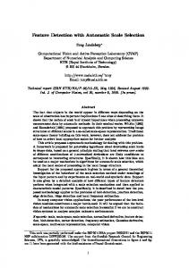
In the case of a cut at frame i, all features should be lost between frames i and i+1. However, there are cases where the pixel areas in the new frame coincidentally match features that were being tracked. In order to prune these coincidental matches, we examine the minimum spanning tree of the tracked and lost feature sets. We can see from Figure 2 (b), in the case of a cut, that a very small percentage of features are tracked. These tracked features are, in fact, erroneous. We can remove some of these erroneous matches by examining properties of the minimum spanning tree (MST) of the tracked and lost feature sets. By severing edges that link tracked features to lost features we end up with several disconnected components within the graph (MST). Any node in the graph that becomes a singleton has its status changed from tracked to lost, and is subsequently included in the lost feature count. The property we are exploiting here the fact that erroneously tracked features will be minimal and sur-
4
Anthony Whitehead, Prosenjit Bose, Robert Laganiere
rounded by lost features. Clusters of tracked (or lost) features therefore have localized support that we use to lend weight to our assessment of erroneous tracking.
(a)
(b)
Fig. 2. Minimum spanning trees for two consecutive frames (+) are tracked features, (X) are lost features. (a) high proportion of successfully tracked features from previous frame (b) features cannot be found in high proportion, indicating a cut. The circle shows erroneous tracking.
Our inter-frame difference metric is the percentage of lost features from frames i to i+1. This corresponds to changes in the minimum spanning tree, but is computationally efficient. Because we are looking to automatically define a linear discriminator between the cut set and the non-cut set, it is advantageous to separate these point sets as much as possible. In order to further separate the cut set from the non-cut set, we square the percent feature loss which falls in the range [0..1]. This has a beneficial property of ensuring the densities of the cut set and the non-cut set are further separated and thus ease the computation of a discriminating threshold. The idea here is that in the case of optimal feature tracking, non-cut frame pairs score 1 (all features tracked) and cut frame pairs score 0, no features tracked. Squaring, in the optimal case, has no effect as we are already maximally separated. However, in practice, squaring forces the normalized values for non-cut frame pairs closer to zero. Figure 3 shows this stretching of the inter-frame differences and how cuts and non-cuts are well separated. Now that we have determined interframe differences, we continue by discussing the classifier.
% Lost Features
1 0.8 0.6 0.4 0.2 0 1
21
41
61
81
101
121
141
161
181
Frame Number
Fig. 3. Cuts expose themselves as high inter-frame feature loss.
Feature Based Cut Detection with Automatic Threshold Selection
3
5
Automatically Determining a Linear Discriminator
There is no common threshold that works for all types of video. Having a difference metric and a method to further separate the cut set from the non-cut set, we can now compute the linear discriminator for the two sets. There are two classes of frame differences, cuts and non-cuts; and our goal is to find the best linear discriminator that maximizes the overall accuracy of the system. The cut set and the non-cut set can be considered to be two separate distributions that should not overlap, however, in practice they often do. When the two distributions overlap, a single threshold will result in false positives and false negatives. An optimal differencing metric would ensure that these two distributions do not overlap; in such a case the discriminating function is obvious and accuracy is perfect. Figure 4 demonstrates this. The quality of the difference metric directly affects the degree to which the two distributions overlap, if any; and until an optimal difference metric is proposed, the problem of optimal determination of the discriminator must be considered. We have opted to examine the density of the squared inter-frame difference values for an entire sequence. The idea here is that there should be two distinct high-density areas, those where tracking succeeded (Low feature loss) and those where tracking failed (high feature loss). In practice, this situation appeared about 50% of the time in our data set. We will introduce the idea of a candidate set in section 3.2, which is the set of features that can be discriminated by zero crossings of the probability density function that characterizes the densities of the inter-frame differences. It needs to be noted here that while we examine the density for the entire sequence to determine a global threshold, it is possible to apply the method outlined next in a windowed manner to determine localized thresholds. 3.1
Density Estimation
In order to auto-select a threshold, we examine the frequency of high and low feature loss. We are looking to exploit the fact that the ratio of non-cuts to cuts will be high, and therefore the ratio of low feature loss frame pairs to high feature loss frame pairs will also be high. As the frame to frame tracking of features is independent of all other video frames, we have n independent observations from an n+1 frame video sequence. The extrema of the probability density function (PDF) can be used to determine the threshold to use. We can use the statistical foundations of density estimation to estimate this function. The kernel density estimator for the estimation of the density value f(x) at point x is defined as
1 n xi − x fˆ ( x) = ∑K nh i =1 h h
(1)
Where K(●) is the so-called kernel function, h is the window size, and n is the number of frames. Through a series of experiments, the triangular kernel (K(α) = 1- |α|) was selected because it did not over-smooth locally, making the determination of extrema
6
Anthony Whitehead, Prosenjit Bose, Robert Laganiere
easiest. Kernel widths of 7 have provided good results in our experiments. The PDF can be estimated in linear time because we have a small histogram with only 101 bins. 3.2
The Candidate Sets
Non-overlapping sets of distributions are very easily determined by looking for a large plateau of zero density as in Figure 4(a). The first appearance of a large plateau of zero density indicates the range of the separation point. Selecting the extreme end point (closest to the cut set) for the threshold has yielded the correct result on all cases of non-overlapping distributions in our test suite. In practice, the problem is not so simple. We next introduce the ideas around what we term the candidate sets.
Max Max Max Recall F1-Score Precision D e n s i t y
D e n s i t y % Feature Loss (a)
% Feature Loss (b)
Fig. 4. (a) Non-overlapping distributions of cuts/non-cuts, error free discrimination (b) Overlapping distribution of cuts and non-cuts. Error region outlined in gray, and maximum Recall, Precision and F1 score thresholds pointed out. We define 3 candidate sets, where each set contains the frames that maximize the precision, F1 and recall rates. Precision is the portion of the declared cuts that were correct and is maximized when the non-cut distribution ends. Recall is portion of the cuts that were declared correctly and is maximized when the cut distribution ends. The F1 is a combination of precision and recall and is maximized at the intersection of the two distributions. Figure 4(b) shows the overlapping distributions and the position of the candidate set thresholds. Depending on user need, precision, recall or best overall performance (F1), thresholds for these candidate sets can be determined. The candidate sets are the 3 thresholds that for convenience we will call the precision set (P), the F1 set (F) and the recall set (R). The candidate sets are determined by examining zero crossings of the first derivative of the computed probability density function. There are often many consecutive zero crossings of the function over time, so we use a modified function G(x) to make the large changes in density more apparent. G(x) is defined using the following rules:
G ( x) = g ( x) +g ( x + 1) : if fˆ ′( x) ≤ 0 then g ( x) = 0 if fˆ ′( x) > 0 then g ( x) = 1
(2)
Feature Based Cut Detection with Automatic Threshold Selection
7
The zero crossings are determined by starting from 100 percent feature loss and examining G(x) as x (% feature loss) decreases. • (P) is the first zero crossing • (F) The position of the minimum of PDF corresponding to the plateau of G(x) given: o If the next zero crossing has opposing direction as the first and is part of the plateau of first zero crossing use this plateau (i.e. is u or n shaped), otherwise use the next plateau. • (R) The next subsequent zero crossing
The arrows in Figure 5(b) point to the zero crossings computed using the rules. The first zero crossing is at 98 (P) and because the next zero crossing at 93 is also an upwards direction (u shaped), we skip to the next plateau to determine F. The next zero crossing (not on the plateau) is used for R. 0.006 0.005
Density
0.004 0.003 0.002 0.001 0 0.6
0.65
0.7
0.75
0.8
0.85
0.9
0.95
1
0.95
1
Percent Feature Loss (a) 2 1.5 1
F
G(x)
0.5 0 -0.5 -1
0.6
0.65
0.7
0.75
0.8
0.85
0.9
R
P
-1.5 -2
Percent Feature Loss (b)
Fig. 5. (a) original PDF (b) Modified first derivative (G(x))
8
5
Anthony Whitehead, Prosenjit Bose, Robert Laganiere
Experimental Results
In the experiment that follows, a selection of video clips that represent a variety of different video genres are used. The data set was specifically selected based on characteristics that cause difficulties with known methods. In particular, we selected clips with fast moving objects, camera motions, highly edited and various digitization qualities and lighting conditions. We compare the results of the proposed method against a pixel-based method with relative localization information and a histogram based method [12]. For the proposed method, we ran each sample through the system once and computed the F1 candidate set threshold as outlined in Section 4. For the two comparison methods, we preformed binary search to find the maximum F1 score. Table 1. Results on data set.
Proposed feature tracking method
Pixel Based method with localization
Histogram MethodCut Det (MOCA)
Data Source
Precision
Recall
F1
Precision
Recall
F1
Precision
Recall
F1
A B C D E F G H I J AVG VAR DEV
1 1 .595 1 .938 1 .810 .895 1 .497 .874 .034 .185
1 1 .870 1 1 1 .944 .895 1 .897 .961 .003 .054
1 1 .707 1 .968 1 .872 .895 1 .637 .908 .018 .134
1 .825 .764 1 .867 0 .708 .927 1 .623 .774 .090 .301
1 .825 .778 1 .867 0 .994 1 1 .540 .800 .101 .318
1 .825 .771 1 .867 0 .809 .962 1 .591 .783 .093 .304
1 1 .936 1 .955 1 1 .971 1 .850 .971 .002 .048
1 .375 .536 .941 .700 1 .667 .895 .500 .395 .701 .060 .246
1 .545 .682 .969 .808 1 .800 .932 .667 .540 .794 .036 .190
In Table 1, we present the results of running the 3 methods on the dataset. The proposed method outperforms both the histogram-based method and the pixel based methods. In most cases (8 of 10) the proposed method provides the best achievable F1 score. A simple statistical analysis of the overall capabilities is given at the end of Table 1. The average, variance and standard deviation for the 10 samples were computed. On average, the proposed method significantly outperforms the other two methods. The variance and the standard deviation show that the results offered by the proposed method are also more stable across a variety of different video genre. It is not surprising that ‘cutdet’ out performs the proposed system in H, because the abstract was created by the MOCA project, however it is surprising that the pixel based method outperformed both. In examples C and J, the F1 score was not maximized as the heuristic to determine the F1 candidate set threshold did not achieve the best value, rather a good value. Within the range of the F1 candidate set threshold plateau,
Feature Based Cut Detection with Automatic Threshold Selection
9
maximum F1 was achievable. For all the experiments we tracked 100 features with a minimum feature disparity of five pixels. The processing time for a frame pair is slightly less than 70 ms on a 2.2 GHz Intel processor on frames sized 320x240 pixels.
6
Conclusions
We have presented a feature-based method for video segmentation, specifically cut detection. By utilizing feature tracking and an automatic threshold computation technique, we were able to achieve F1, recall and precision rates that generally match or exceed current methods for detecting cuts. The method provides significant improvement in speed over other feature-based methods and significant improvement in classification capabilities over other methods. The application of feature tracking to video segmentation is a novel approach to detecting cuts. We have also introduced the concept of candidate sets that allow the user to prejudice the system towards results meeting their individual needs. This kind of thresholding is a novel approach to handling the overlapping region of two distributions, namely the cut set and the noncut set in video segmentation. Space constraints prevented the complete description and further information is available in a full and complete technical report. Please contact the authors to access the technical report.
References 1. A. Seyler: Probability distribution of television frame difference, Proc. Institute of Radio Electronic Engineers of Australia 26(11), pp 355-366, 1965 2. J. Lee and B. Dickinson: Multiresolution video indexing for subband coded video databases, in Proc. Conference on Storage and Retrieval for Image and Video Databases, 1994. 3. R. Lienhart: Dynamic Video Summarization of Home Video, SPIE Storage and Retrieval for Media Databases 2000,. 3972, pp. 378-389, Jan. 2000. 4. R. Lienhart, S. Pfeiffer, and W. Effelsberg: Video Abstracting. Communications of the ACM, Vol. 40, No. 12, pp. 55-62, Dec. 1997. 5. M. M. Yeung and B.-L. Yeo: Video Visualization for Compact Presentation and Fast Browsing of Pictorial Content. IEEE Trans. on Circuits and Systems for Video Technology, Vol.7, No. 5, pp. 771-785, Oct. 1997. 6. A. Hampapur, R. Jain, and T. E. Weymouth: Production Model Based Digital Video Segmentation. Multimedia Tools and Applications, Vol.1, pp. 9-45, 1995. 7. R. Lienhart: Reliable Transition Detection In Videos: A Survey and Practitioner's Guide. International Journal of Image and Graphics (IJIG), Vol. 1, No. 3, pp. 469-486, 2001. 8. R Zabih, J. Miller, and K. Mai: A Feature-Based Algorithm for Detecting and Classifying Scene Breaks, Proc. ACM Multimedia, pp. 189-200, 1995 9. R Zabih, J. Miller, and K. Mai: A Feature Based Algorithm for detecting and Classifying Production Effects, Multimedia Systems, Vol 7, p 119-128, 1999. 10. A Smeaton et al.: An Evaluation of Alternative Techniques for Automatic Detection of Shot Boundaries in Digital Video, in Proc. Irish Machine Vision and Image Processing, 1999. 11. B. Lucas and T. Kanade: An Iterative Image Registration Technique with an Application to Stereo Vision, Int. Joint Conference On Artificial Intelligence. pp 674-679, 1981. 12. S. Pfeiffer, R.Lienhart, G. Kühne, W. Effelsberg: The MoCA Project - Movie Content Analysis Research at the University of Mannheim, Informatik '98, pp. 329-338, 1998.