FPGA Implementation of a Recurrent Neural Fuzzy Network with On ...

JOURNAL OF INFORMATION SCIENCE AND ENGINEERING 25, 575-589 (2009)

FPGA Implementation of a Recurrent Neural Fuzzy Network with On-Chip Learning for Prediction and Identification Applications* CHENG-JIAN LIN AND CHI-YUNG LEE+ Department of Computer Science and Information Engineering National Chin-Yi University of Technology Taichung County, 411 Taiwan + Department of Computer Science and Information Engineering Nankai University of Technology Nantou County, 542 Taiwan In this paper, a hardware implementation of a recurrent neural fuzzy network (RNFN) used for identification and prediction is proposed. A recurrent network is embedded in the RNFN by adding feedback connections in the second layer, where the feedback units act as memory elements. Although the back propagation (BP) learning algorithm is widely used in the RNFN, BP is too complicated to be implemented using hardware. However, we use the simultaneous perturbation method as a learning scheme for hardware implementation to overcome the above-mentioned problems. The hardware implementation of the RNFN uses random access memory (RAM), which stores all the parameters of a network. This design method reduces the number of logic gates used. The major findings of the experiment show that field programmable gate arrays (FPGA) implementation of the RNFN retains good performance in identification and prediction problems. Keywords: recurrent neural fuzzy network (RNFN), field programmable gate array (FPGA), simultaneous perturbation learning, random access memory (RAM), prediction, identification

1. INTRODUCTION Implementation of the recurrent neural fuzzy networks (RNFN) [1-4] is usually simulated using software, but the processing speed using software is not fast enough to meet the demand of real time. Therefore, we propose implementing RNFN using hardware. Implementation of neural networks using hardware has been successfully implemented before. Krips [5] proposed using field programmable gate arrays (FPGA) to implement neural networks through parallel computing in real-time hand-tracking systems. Mohd-Yasin [6] realized IRIS recognition for biometric identification employing neural networks in FPGA devices, which enable efficient hardware implementation. Hardware implementation of the RNFN with learning ability is a very difficult issue. The back propagation (BP) learning method is widely used in the RNFN. But BP is difficult to implement using hardware because of the difficulty of calculating the back propagation error of all the parameters in the system. However, we use the modified simultaneous perturbation method [7, 8] as a learning strategy for hardware implementaReceived May 8, 2007; revised November 6, 2007, May 21 & July 15, 2008; accepted August 22, 2008. Communicated by Yao-Wen Chang. * This work was supported by the National Science Council of Taiwan, R.O.C., under grant No. NSC 97-2221E-167-022.

575

576

CHENG-JIAN LIN AND CHI-YUNG LEE

tion. In [19], Maeda and Wakamura described a recursive learning scheme for recurrent neural networks using the simultaneous perturbation method. Unlike ordinary correlation learning, this method is applicable to analog learning and to the learning of oscillatory solutions of recurrent neural networks. Moreover, as a typical example of recurrent neural networks, Maeda and Wakamura considered the hardware implementation of Hopfield neural networks using a field-programmable gate array (FPGA). Our proposed method is similar to this study, but it has some differences in the application domain. For example, Maeda and Wakamura used Hopfield neural networks, which are different from our methods, which use the RNFN structure. The Hopfield network is not trained in the same way as a Multi-Layer Perceptron (MLP) network. And the topology of Hopfield network differs from those of the MLP. There are no distinct layers. Every unit is connected to every other unit. In addition, the connections are bi-directional (information flows in both directions along them), and symmetric. There is a single weight assigned to each connection that is applied to data moving in either direction. Specifically, the characteristics of the networks are different. Neural fuzzy networks bring the low-level learning and computational power of neural networks to fuzzy systems and provide the highlevel human-like thinking and reasoning capability of fuzzy systems to neural networks. In this paper, hardware implementation of the RNFN uses random access memory (RAM) which stores all the parameters of the RNFN. This strategy reduces the number of logic gates for the parameters and fuzzy logic rules of the RNFN. Development of digital integrated circuits for use as field programmable gate arrays (FPGA) makes the hardware designing process flexible and programmable. From the perspective of computer-aided design, FPGA has the merits of lower cost, higher density, and shorter design cycle. In this paper, we propose realizing the hardware implementation of the RNFN structure on a FPGA chip. In our method, we use VHDL (very high speed integrated circuit hardware description language) to realize the RNFN with the simultaneous perturbation learning algorithm. The advantages of the proposed method are summarized as follows: (1) The hardware implementation of a recurrent neural fuzzy network (RNFN) is proposed for prediction and identification problems. We use the modified simultaneous perturbation method as a learning scheme for hardware implementation to overcome the complex operation problems of a learning algorithm. (2) We adopt a second order non-linear function to implement the Gaussian function to reduce the chip area. (3) The proposed hardware implementation of the RNFN uses random access memory (RAM) to store all the parameters of a network. The design method can reduce the number of used logic gates. (4) We use very high speed integrated circuit hardware description language (VHDL) to design RNFN with learning ability and to implement it on field programmable gate arrays (FPGA).

2. STRUCTURE OF THE RNFN MODEL The recurrent neural fuzzy network (RNFN) [3, 9] realizes a fuzzy model in the following form:

FPGA IMPLEMENTATION OF A RECURRENT NEURAL FUZZY NETWORK

Rule-j: [ IF h1j is A1j and h2j is A2j…and hNj is ANj], THEN y′ is wj

577

(1)

where, hij = xi + uij(2) (t − 1) ⋅ θij , for i = 1, 2, …, N, y′ is the output variable, Aij is the linguistic term of the precondition part, wj is the constant consequent part, N is the number of input variables, and θij is the link weight of the feedback unit. Next, we describe the operation functions of the nodes in each layer of the RNFN model. u(l) denotes the output of a node in the lth layer. No computation is done in Layer 1. Only transmits input values to the next layer directly, i.e. ui(1) = xi . . The Gaussian membership function, the operation performed in Layer 2, is ⎛ [hij − mij ]2 uij(2) = exp ⎜ − ⎜ σ ij 2 ⎝

⎞ ⎟ ⎟ ⎠

(2)

where mij and σij are, respectively, the mean and variance of the Gaussian membership function of the jth term of the ith input variable xi. In addition, the inputs of this layer for discrete time t can be defined as hij (t ) = ui(1) (t ) + uij(2) (t − 1) ⋅ θij

(3)

where uij(2) (t − 1) denotes the feedback unit of memory which stores the past information of the system and where θij denotes the link weight of the feedback unit. Layer 3 is denoted by ∏, which multiplies the incoming signals and outputs the product result. As a result, the output function of each inference node is ⎛ (2) ⎞ u (3) j = ⎜ ∏ uij ⎟ ⎝ i ⎠

where the

∏ uij(2)

(4)

of a rule node represents the firing strength of its corresponding rule.

i

The node in Layer 4 is labeled ∑, and it sums all incoming signals to obtain the final inferred result uk(4) = ∑ u (3) j w jk , where the weight wjk is the output action strength of the j

kth output associated with the jth rule, and uk(4) is the kth output of the RNFN. Finally, the overall representation of input x and the kth output is R ⎧⎪ N ⎡ [ui(1) (t ) + uij(2) (t − 1) ⋅ θij − mij ]2 ⎤ ⎫⎪ ⎥⎬ yk (t ) = uk(4) (t ) = ∑ w jk ⎨∏ exp ⎢ − σ ij 2 ⎢⎣ ⎥⎦ ⎪⎭ j =1 ⎪⎩ i =1

(5)

where ui(1) = xi , mij, σij, θij, and wjk are the tuning parameters, and uij(2) (t − 1) = exp{−[ui(1) (t − 1) + uij(2) (t − 2) ⋅ θij − mij ]2 /(σ ij ) 2 }.


578

Fig. 1. Structure of the RNFN.

3. THE MODIFIED SIMULTANEOUS PERTURBATION ALGORITHM FOR RNFN LEARNING When this study utilizes the gradient descent method as a learning algorithm to train a RNFN, the parameters are updated iteratively. First, this study defines a cost function as follows J (u ) =

1 ( y − yd ) 2 , 2

(6)

where yd and y are the desired output and the current output, respectively. The optimization target is characterized to minimize the error function with respect to the adjusted parameters u of the RNFN. Then, according to the gradient descent method, the parameters are updated using the chain rule Δu = − η

∂J (u ) ∂J (u ) ∂y ∂y ∂y = −η = − η ( y − yd ) = − ηe ∂u ∂y ∂u ∂u ∂u

(7)

where η is the learning rate. In Eq. (7), e, the error between the desired output and the current output, can be calculated easily, but ∂y/∂u requires more complicated computation. Therefore, many researchers [10, 11] used the different approximation approach to obtain a derivation of a function. They added a small perturbation factor c to the ith parameter of the parameter vector, ui = (u1, …, ui + c, …, uk), where k is the number of adjustable parameters. They utilized the different approximation approach to derive ∂y/∂u. This can calculate the amount of parameter modification for the RNFN: Δu = − η

J (ui ) − J (u ) ∂J (u ) ≈ −η . ∂u c

(8)


579

On the other hand, they also utilized the different approximation approach to derive the ∂y/∂u as follows: ∂y f (ui ) − f (u ) ≈ . ∂u c

(9)

Although the different approximation approach is simple, it requires many forward operations in the RNFN. When the number of adjustable parameters is k, k-times forward operations are required to complete the amount of parameter modifications for all parameters. Therefore, when the number of adjustable parameters in the network is large, this approach is not suitable. In order to improve the above-mentioned disadvantages, we adopt a modification of the simultaneous perturbation method [7, 8] for RNFN learning. First, we define a perturbation vector that is added to all parameter of the RNFN, cl = (c1l , … , cln ), where l denotes an iteration. The modified simultaneous perturbation learning rule is as follows: Δwli = − η el Δmli = − η el Δσ li = − η el

Δθli = − η el

f ( pl + cl ) − f ( pl ) i cwl

f ( pl + cl ) − f ( pl ) i cml

f ( pl + cl ) − f ( pl ) cσi

(11) (12)

l

f ( pl + cl ) − f ( pl ) cθi

(10)

(13)

l

where el = (yl − ydl), in which el is an error between the actual output of the system and the desired output, η is a positive learning rate parameter for all parameters of the RNFN, f(pl + cl) is the output of the RNFN which adds the perturbation vector to all parameters, i , pl is the parameter vector, and cl is the perturbation vector. The perturbation vector cwl i i i cml , cσ l and cθ l are a uniformly random number in the interval [− cmax, cmax], except in the interval [− cmin, cmin] and is independent with respect to time l for i = 1, …, n.

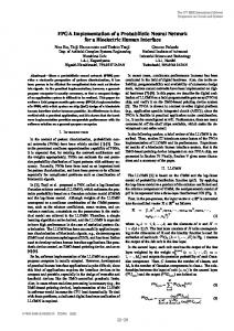
4. IMPLEMENTATION OF THE RNFN USING FPGA Fig. 2 shows the general layout and data flow diagram of the RNFN. It consists of seven major units: (1) a Gaussian function unit; (2) an inference processing unit; (3) a defuzzifier unit; (4) a comparison block; (5) a learning block; (6) a parameter update unit; and (7) a controller. 4.1 Data Representation

In this study, we use a fixed-point number for RNFNs to maintain consistency and effectiveness of the representation of data which are the same. The encoding technique


580

clk reset clk

clk reset

Controller

reset

clk

clk reset

reset

u(3)

Inference Processing Unit

u(4)

Defuzzifier Unit

en

en

u(2)

u(2) (t-1)

Gaussian Function Unit

y yd

Compare Block error

en

en

ｗ

Desired output

en

en

Parameter Modification Unit

Learning Block △ｍ、△σ、△θ、△ｗ

ｍ、σ、θ

Input

Fig. 2. Data flow diagram of the RNFN model.

Table 1. Data representation. Value 8 4 2 1 0.5 0.25 0.0125 0.0625 0.03125

0 0 0 0 0 0 0 0 0

Data representation Format: s4·11 1000 00000000000 0100 00000000000 0010 00000000000 0001 00000000000 0000 1000000000 0000 0100000000 0000 0010000000 0000 0001000000 0000 0000100000

uses digital values as a means to represent the respective data [12, 13]. The fixed-point format is defined as follows: [s] a·b

(14)

where the optional s denotes a sign bit with 0 for positive numbers and 1 for negative numbers, a is the number of integer bits, and b is the number of fractional bits. Table 1 shows the principal values with the above-mentioned technique. Table 1 shows that the fixed-point numbers are easily accommodated in this system. Therefore, the smallest value can be represented by − 15.999023 (1 1111 11111111111) and the largest value by 15.999023 (0 1111 11111111111). For all practical systems it is possible to choose a word-length long enough to reduce the finite precision effects in a negligible level, and it is often desirable to use as few bits as possible while achieving user-defined output error conditions in order to optimize area, power, or speed [14, 15]. This study uses 16 bits as the number of word-length for all operations.


581

4.2 Random Access Memory Unit

In order to reduce the number of logic gates for the fuzzy rules and parameters, we use the Random Access Memory (RAM) method [16]. The main advantage of the RAM method is its ability to access parameter values (w, m, σ, θ) in each layer in the RNFN. The RAM method can greatly reduce the number of logic gates. The RAM module is generated based on the user-specified width and depth. The input and output data of a bit number represent the width, and the address of a parameter number used in the network represents the depth. The structure of a RAM is shown in Fig. 3. The RAM implementation supports three different write mode options that determine the behavior of the data output port during a write operation. These three different operation modes are as follows: 1. Read-After-Write (Write First): The data input is loaded simultaneously with a write operation on the Dout port. The data input is stored in the RAM and mirrored on the output. 2. Read-Before-Write (Read First): In this mode, data previously stored in the write address appears on the output latches. Data input is stored in the RAM and the prior content of that location is driven on the output during the same clock cycle. 3. No-Read-On-Write (No Change): The Dout port remains unchanged during a write operation. The data output is still the last read data and is unaffected by a write operation on the same port.

Fig. 3. The RAM structure.

4.3 Gaussian Function Unit

The main purpose of the Gaussian function unit in the RNFN is to correspond to one linguistic label of the input variables in Layer 1 and to a unit of memory. The membership value specifying the degree to which an input value belongs to a fuzzy set is calculated in Layer 2. The Gaussian function is the main part of the structure of the NFN for the fuzzy rules. In Eq. (2), we know that the operator of the Gaussian function is very complicated using the traditional non-linear activation functions. The Taylor series with a look-up table (LUT) has been adopted to approximate the implementation of the Gaussian function. The method requires a quite large number of hardware resources. Therefore, it is unsuitable for direct digital implementation in hardware. A reasonable approximation of a nonlinear function can be implemented directly using digital techniques. The following equation is a second order non-linear function [13]:


582

⎧( z ⋅ ( β − θ ⋅ z ) + 1) / 2 for 0 ≤ z ≤ L F ( z) = ⎨ ⎩( z ⋅ ( β + θ ⋅ z ) + 1) / 2 for − L ≤ z ≤ 0

(15)

where β and θ represent the slope and the gain of the non-linear function F(z) between the saturation regions – L and L. Taking the upper and lower saturation regions to be equal to 2, we get the expressions for θ and β as:

θ =±

1 and β = 1. 4

As shown in Fig. 4, the RNFN is added to a feedback unit in the Gaussian function. The implementation of the feedback unit in the Gaussian function is stored in a register. In our implementation, in order to reduce the number of logic gates for fuzzy rules and parameters, we used the RAM in the hardware implementation of the RNFN to obtain a configurational structure of the hardware. The four parameters (w, m, σ, θ) of the Gaussian function unit are stored in the RAM. The depth is used to represent the fuzzy rule number used in the Gaussian function, and the width is used to represent the data bit number of the parameters. For example, if 12 fuzzy rule numbers are used in the Gaussian function unit, the depth in the RAM is the number of 12 fuzzy rules, and the width in the RAM is the 16 bits of the input data. In Fig. 4, X is an input value of the Xth input node in Layer 1. The enable pin is the main pin that controls the Gaussian function, and the role of the Gaussian function is to confirm whether all input data (X, Y(k), w, m, σ, θ) are accessed or calculated.

Fig. 4. Hardware implementation of the Gaussian function.

4.4 The RAM Learning Unit

Fig. 5 shows the RAM learning unit. The modifying quantity of all the parameters is represented by Eqs. (10) to (13). The perturbation value is added to each parameter. As a result, each parameter has different modifying quantities and can be updated. The perturbation value is a uniformly random number in an [− cmax, cmax] interval except in the interval [− cmin, cmin]. Random number generation uses a Linear Feedback Shift Register (LFSR). Using LFSR counters to address the register makes the design even simpler. An n-bit LFSR counter can have a maximum sequence of 2n − 1 states. The RAM learning unit is a structure of a single output system, as shown in Fig. 5. The f(pl + cl) − f(pl) is the


583

Fig. 5. The RAM learning unit of a single output system.

error between the output of the RNFN without perturbation and the output of the RNFN with perturbation at the beginning. We can find the error (el) between the output of the RNFN without perturbation and the desired output. Next, the two errors (i.e., f(pl + cl) − f(pl) and el) and the learning rate (η) are sent to the multiplier. Therefore, η × el × (f(pl + cl) − f(pl)) is sent to the divider and calculated with the perturbation value of the register. The modifying quantity we obtain is written into the RAM. 4.5 RAM Parameter Modification Part

The RAM parameter modification part, which modifies quantities through the RAM learning unit, can update the parameters in a network. A block diagram of the RAM parameter modification part is shown in Fig. 6. The parameters of the RNFN (w(k), m(k), σ(k), and θ(k)) and the modified quantities (Δw(k), Δm(k), Δσ(k), and Δθ) perform an addition operation. In this figure, when the parameters are refreshed, the original ways to express the data will exceed the predefined values and result in overflow. This leads to problems when the parameters are refreshed. We have also included a limiter in the refresher which restricts the numerical value of the parameters in the range [− 16, + 16].

Δw(k )

Δw(k )

Fig. 6. The RAM parameter modification part.

The method for the control of data in the RAM parameter modification part is explained as follows:

584


Step 1: The modified quantity RAM and the weight RAM appoint an address of parameters. When the read/write signal is “0,” the RAM will perform the read action. Step 2: The modified quantity RAM and the weight RAM read Δwn(k) and Δwn(k) separately from the RAM and send them to an adder for calculation. Step 3: After calculation by the adder, the output of the adder will be sent to a limiter which decides whether an overflow occurs and which restricts the numerical value of the parameters in the range [− 16, + 16]. Step 4: Finally, the parameter wn(k + 1) is updated and sent back to the weight RAM. When the read/write is signal “1”, the RAM will perform the write action. Step 5: After a new parameter is written, steps 1 to 4 are repeated and the address of the RAM will be changed.

5. EXPERIMENTAL RESULTS This section discusses using the prediction of a time sequence and the identification of a dynamic system to verify the hardware implementation of the RNFN with learning ability. The results of the design of the FPGA chip were checked and configured using the XILINX ISE6.2i and Modelsim 5.7g software. The chip circuit used was Xilinx Virtex-II XC2V6000-4FF1152C. The chip is composed of 6,000,000 system gates, and its clock rate was set to 50-MHz for these examples. The perturbation c is a uniformly random number in the interval [− 0.01, 0.01] except in the interval [− 0.001, 0.001]. Example 1: Prediction of Time Sequence To verify whether the proposed RNFN can learn temporal relationships, a simple time sequence prediction problem found in [17] was used in the example. In this example, the RNFN contained only two input nodes, which were activated with the two dimensional coordinate of the current point, and two output nodes, which represented the two dimensional coordinate of the predicted point. In training the RNFN, we used 6000 learning iterations. Each comprises 12 training data. A learning rate of η = 0.00244140625 was chosen for the hardware. Initial parameters were random in the interval [0, 1]. The random number generation part used a linear feedback shift register (LFSR). Besides, we adopt a root-mean-square (RMS) error to evaluate the performance of various rule num1 Nt ∑ ( yk − yk )2 , where yk repreNt k =1 sents the model output of the kth data, yk represents the desired output of the kth data, and Nt represents the number of the training data. In this example we adopted 12 fuzzy logic rules for the hardware and software implementation of the RNFN. The learning time with the hardware implementation cost about 1.8 seconds. The learning time with the software implementation cost about 3 seconds. The hardware implementation of the RNFN with 12 fuzzy logic rules needed to use about 189,000 logic gates. The peak memory usage was about 64k bits of RAM. The comparisons of resource requirement of various neural networks hardware implementation are shown in Table 2. Although the utilized resource of implement of our model has more support than the NFN model and NN model, structures of the NFN model and NN model are much simpler.

bers. The RMS error is defined as RMS error =


585

Table 2. Comparisons of resource requirement of various neural networks hardware implementation in Example 1. Device Selected FEATURES Number of Slices Number of Slice Flip Flops Number of 4 input LUTs Number of bonded IOBs Number of MULT18X18s Number of GCLKs Memory usage

RNFN 7194 825 12953 347 16 1 64k bits

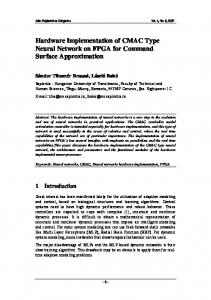
Fig. 7. Prediction results of the RNFN output using software implementation.

XC2V6000 NFN[20] WRFNN[18] 6512 9799 755 1450 11035 14748 461 187 14 60 1 1 52k bits 75k bits

NN[7] 3670 423 7012 286 55 1 28k bits

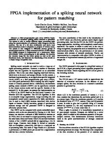
Fig. 8. Prediction results of the RNFN output using FPGA implementation.

Experimental results show that we obtained perfect prediction capability. Fig. 7 shows the prediction results using the software implementation of the RNFN. The figure shows that the RNFN also obtains perfect prediction capability. The prediction results from the hardware implementation of the RNFN are shown in Fig. 8. This figure shows that the results of the hardware and software implementation of the RNFN in prediction problems are similar. Example 2: Identification of a Dynamic System In this example, a nonlinear plant with multiple time delays is guided by the following differential equation [3]:

yp(t + 1) = f(yp(t), yp(t − 1), yp(t − 2), up(t), up(t − 1))

(16)

where f ( x1 , x2 , x3 , x4 , x5 ) =

x1 x2 x3 x5 ( x3 − 1) + x4 1 + x2 2 + x32

(17)

Here, the current output of the plant depends on three previous outputs and two previous inputs. In [18], a feedforward neural network, with five input nodes for feeding the


586

appropriate past values of yp and u, were used. In our model, only two input values, yp(t) and u(t), were fed to the RNFN to determine the output yp(t + 1). The training inputs were independent and had an identically distributed (i.i.d.) uniform sequence over [− 2, 2] for about half of the training time and a single sinusoid signal given by 1.05sin(πt/45) for the remaining training time. There was no repetition of these 900 training data; that is, we had different training sets for each epoch. The check input signal u(t), as shown in the equation below, was used to determine the identification results.

⎧ ⎛π ⋅t ⎞ ⎪sin ⎜ 25 ⎟ ⎠ ⎪ ⎝ ⎪1.0 u (t ) = ⎨ ⎪−1.0 ⎪ ⎛π ⋅t ⎞ ⎛π ⋅t ⎞ ⎛π ⋅t ⎞ ⎪0.3sin ⎜ 25 ⎟ + 0.1sin ⎜ 32 ⎟ + 0.6sin ⎜ 10 ⎟ ⎝ ⎠ ⎝ ⎠ ⎝ ⎠ ⎩

0 < t < 250 250 ≤ t < 500 500 ≤ t < 750

(18)

750 ≤ t < 1000

Table 3. Comparisons of resource requirement of various neural networks hardware implementation in Example 2. Device Selected FEATURES Number of Slices Number of Slice Flip Flops Number of 4 input LUTs Number of bonded IOBs Number of MULT18X18s Number of GCLKs Memory usage

RNFN 5416 2756 9848 167 12 1 50k bits

XC2V6000 NFN[20] WRFNN[18] 4512 8576 683 1120 10102 14748 363 187 14 60 1 1 48k bits 72k bits

NN[7] 3102 376 6132 236 55 1 25k bits

In training the RNFN, we used 2000 learning iterations. Each comprises 900 time steps. The learning rate η = 0.016978125 was used in the hardware implementation of the RNFN. Initial parameters of LFSR were random in the interval [0, 1]. In this example, we adopted 15 fuzzy rules for the hardware and software implementation of the RNFN. The learning time with the hardware implementation required about 42 seconds. The learning time with the software implementation required about 73 seconds. The hardware implementation of the RNFN required approximately 152,000 logic gates, and the peak memory usage was about 50k bits of RAM on a FPGA chip. The comparisons of resource requirement of various neural networks hardware implementation are shown in Table 3. In this table, the results of resource requirement of various networks hardware implementation are similar to Example 1. Experimental results show that the RNFN model has perfect identification capability. Fig. 9 (a) shows the software implementation results of the RNFN for identification. Fig. 9 (b) illustrates the errors between the desired output and the RNFN output from the software implementation. The experimental results demonstrate the dynamic system capability of the RNFN model. Fig. 10 (a) shows the results from the hardware implementation of the RNFN. The errors between the desired output and the RNFN output from hardware implementation are shown in Fig. 10 (b).


587

(a) (b) Fig. 9. (a) Prediction output and (b) prediction error using RNFN model with software implementation.

(a) (b) Fig. 10. (a) Prediction output and (b) prediction error using RNFN model with FPGA implementation.

6. CONCLUSION A hardware implementation of a recurrent neural fuzzy network (RNFN) with simultaneous perturbation learning algorithm was proposed in this paper. In order to reduce the number of logic gates, we use random access memory (RAM) to store all the parameters of the RNFN for hardware implementation. From the examples given, the results of these performances successfully confirm the validity of using FPGA implementation of the RNFN with a learning scheme to solve temporal prediction and dynamic system identification problems. The simultaneous perturbation algorithm for the RNFN with simple hardware implementation is not suitable because it is likely to get trapped in the local minimum. In the future work, we will use the genetic algorithm or particle swarm algorithm to find the global optimum.

588


REFERENCES 1. C. J. Lin and Y. C. Hsu, “Reinforcement hybrid evolutionary learning for recurrent wavelet-based neuro-fuzzy systems,” IEEE Transactions on Fuzzy Systems, Vol. 15, 2007, pp. 729-745. 2. C. F. Juang, “A TSK-type recurrent fuzzy network for dynamic systems processing by neural network and genetic algorithms,” IEEE Transactions on Fuzzy Systems, Vol. 10, 2002, pp. 155-170. 3. C. J. Lin and C. H. Chen, “Identification and prediction using recurrent compensatory neuro-fuzzy systems,” Fuzzy Sets and Systems, Vol. 150, 2005, pp. 307-330. 4. P. A. Mastorocostas and J. B. Theocharis, “A recurrent fuzzy-neural model for dynamic System Identification,” IEEE Transactions on Systems, Man, and Cybernetics, Vol. 32, 2002, pp. 176-190. 5. M. Krips, T. Lammert, and A. Kummert, “FPGA implementation of a neural network for a real-time hand tracking system,” in Proceedings of the 1st IEEE International Workshop on Electronic Design, Test and Applications, Vol. 29-31, 2002, pp. 313-317. 6. F. Mohd-Yasin, A. L Tan, and M. I. Reaz, “The FPGA prototyping of IRIS recognition for biometric identification employing neural network,” in Proceedings of the 16th International Conference on Microelectronics, 2004, pp. 458-461. 7. Y. Maeda and R. J. P. De Figueiredo, “Learning rules for neuro-controller via simultaneous perturbation,” IEEE Transactions on Neural Networks, Vol. 8, 1997, pp. 1119-1129. 8. Y. Maeda and Y. Kanata, “Learning rules for recurrent neural networks using perturbation and their application to neuro-control,” IEICE Transactions of the Institute of Electrical Engineers of Japan., Vol. 113-C, 1993, pp. 402-408. 9. C. H. Lee and C. C. Teng, “Identification and control of dynamic systems using recurrent fuzzy neural networks,” IEEE Transactions on Fuzzy Systems, Vol. 8, 2000, pp. 349-366. 10. Y. Maeda, “Learning rule of neural networks for inverse systems,” Electron Communication. Japan, Vol. 76, 1993, pp. 17-23. 11. J. C. Spall, “A stochastic approximation technique for generating maximum likelihood parameter estimates,” in Proceedings of the American Control Conference, 1987, pp. 1161-1167. 12. M. T. Tommiska, “Efficient digital implementation of the sigmoid function for reprogrammable logic,” Computers and Digital Techniques, Vol. 150, 2003, pp. 403411. 13. J. J. Blake and L. P. Maguire, “The implementation of fuzzy systems, neural networks and fuzzy neural networks using FPGAs,” Information Sciences, Vol. 112, 1998, pp. 151-168. 14. C. Inacio and D. Ombres, “The DSP decision: Fixed point or floating?” IEEE Spectrum, Vol. 33, 1996, pp. 72-74. 15. C. T. Ewe, P. Y. K. Cheung, and G. A. Constantinides, “Dual fixed-point: An efficient alternative to floating-point computation,” Lecture Notes in Computer Science, Vol. 3203, 2004, pp. 200-208. 16. http://www.xilinx.com, DS234, April 28, 2005.


589

17. S. Santini, A. D. Bimbo, and R. Jain, “Block-structured recurrent neural networks,” Neural Networks, Vol. 8, 1994, pp. 306-319. 18. C. J. Lin and C. C. Chin, “Prediction and identification using wavelet-based recurrent fuzzy neural networks,” IEEE Transactions on Systems, Man, and Cybernetics, Part B: Cybernetics, Vol. 34, 2004, pp.2144-2154. 19. Y. Maeda and M. Wakamura, “Simultaneous perturbation learning rule for recurrent neural networks and its FPGA implementation,” IEEE Transactions on Neural Networks, Vol. 16, 2005, pp. 1664-1672. 20. C. T. Chao, T. J. Chen, and C. C. Teng, “Simplification of fuzzy-neural systems using similarity analysis,” IEEE Transactions on Systems, Man, and Cybernetics. Vol. 26, 1996, pp. 344-354. Cheng-Jian Lin (林正堅) received the Ph.D. degree in Electrical and Control Engineering from the National Chiao Tung University, Taiwan, R.O.C., in 1996. Currently, he is a full Professor of Computer Science and Information Engineering Department, National Chin-Yi University of Technology, Taichung County, Taiwan, R.O.C. His current research interests are soft computing, pattern recognition, intelligent control, image processing, bioinformatics, and FPGA design.

Chi-Yung Lee (李繼永) received the M.S. degrees in Industrial Education from the National Taiwan Normal University, Taiwan, R.O.C., in 1989. Currently, he is an Associate professor of Computer Science and Information Engineering Department, Nan-Kai Institute of Technology, Nantou, Taiwan, R.O.C. His current research interests are neural networks, fuzzy systems, intelligent control, and FPGA design.