WSEAS TRANSACTIONS on SYSTEMS and CONTROL
Trihastuti Agustinah, Achmad Jazidie, Mohammad Nuh
Fuzzy Tracking Control Based on H∞ Performance for Nonlinear Systems TRIHASTUTI AGUSTINAH, ACHMAD JAZIDIE, MOHAMMAD NUH Electrical Engineering Department Institut Teknologi Sepuluh Nopember Kampus ITS Sukolilo Surabaya 60111 INDONESIA
[email protected] Abstract: - This paper presents a fuzzy tracking control design based on H∞ performance for nonlinear systems. The Takagi-Sugeno fuzzy model is employed to approximate a nonlinear system. Based on the H∞ tracking performance, the nonlinear system output is controlled to track a reference signal, and at the same time the tracking performance is attenuated to a prescribed level. Linear matrix inequalities (LMI) techniques are used to solve the fuzzy tracking control problem. The proposed method has been applied to control of a laboratory pendulum-cart system. Hence, the performance has been evaluated in simulations as well as in real-time control.
Key-Words: - Fuzzy tracking control, H∞ performance, LMI, Pendulum-cart system conventional H∞ control scheme are not suitable for practical control system design [6]. In the work of Tseng [4], a fuzzy tracking control design method with a guaranteed H∞ model reference tracking control scheme is proposed to systematically design for continuous-time systems. The proposed design is applied for the multi input multi output (MIMO) systems. However, the application of the design for single input multi output systems, we have to make adjustment on the structure of reference model. Despite the fact that much progress has been made in studying the tracking problem of nonlinear systems, it is still a challenge to apply the control system to the real plant. For practical control design, a simple fuzzy tracking control design with guaranteed control performance is more appealing for nonlinear systems. In this work, the T-S fuzzy model is used to describe the dynamics of the nonlinear system. Then, a fuzzy tracking controller is introduced to track a reference signal, and the H∞ tracking performance is guaranteed for a prescribed level for all external disturbance and reference signal. The LMI convex programming technique is used to solve this problem. The proposed technique is validated by means of a laboratory experiment; a pendulum-cart system. The paper is organized as follows. Section 2 addresses the problem formulation. The H∞ tracking control design is discussed in Section 3. In Section 4, the application of the proposed method in
1 Introduction The Takagi-Sugeno (T-S) fuzzy model has become popular because of its efficiency in controlling nonlinear systems. The T-S fuzzy model has been proved to be a good representation for a class of nonlinear systems [1]. The main property of T-S fuzzy model is to describe the local dynamics by linear models. The overall model of the nonlinear system is obtained by fuzzy blending of these linear models through nonlinear fuzzy membership functions. The tracking control design based on the TakagiSugeno fuzzy model has been treated by several researchers, for instance, Ma [2], Zhang [3], Tseng [4], and Uang [5]. The most important issue for fuzzy tracking control systems is that the output of the nonlinear system tracks a reference signal. In Ma [2], the tracking problem of nonlinear systems is solved using a synthesis of the fuzzy control theory and the linear multivariable control theory. Simulation results show that the proposed tracking control system can make the output of the system to asymptotically track the reference signal. The robust fuzzy tracking controller based on internal model principle is introduced to track a reference signal in [3]. Simulation results on the inverted pendulum system show that the stepwise signal for uncertain nonlinear system can be tracked via the proposed method. The nonlinear H∞ control schemes have been introduces to deal with the robust performance design problem of nonlinear systems. In general,
ISSN: 1991-8763
393
Issue 11, Volume 6, November 2011
WSEAS TRANSACTIONS on SYSTEMS and CONTROL
Trihastuti Agustinah, Achmad Jazidie, Mohammad Nuh
pendulum-cart system is derived. Also, the simulation and experiment results are provided in this section. Finally, Section 5 concludes this paper.
hi ( z (t )) =
µi ( z (t )) L
∑ µi ( z (t )) i =1
z (t ) = [ z1 (t ), z2 (t ),⋯, z g (t )]
2 Problem Formulation The main feature of Takagi–Sugeno fuzzy models is to represent the nonlinear dynamics by linear model according to the so-called fuzzy rules and then to blend all the linear models into an overall single model through nonlinear fuzzy membership functions [7]. The ith rule of the fuzzy model is of the following form:
and where Fij(zj(t)) is the grade of membership function of zj(t) in Fij. It assumed that
µi ( z (t )) ≥ 0 , and
i =1
for all t. Therefore, we get [7], [8]
Plant Rule i:
hi ( z (t )) ≥ 0,
If z1(t) is Fi1 and ··· and zg(t) is Fig
x(t ) ∈ R n×1
u (t ) ∈ R
m×1
denotes
the
state
vector,
denotes the bounded external disturbance, y (t ) ∈ R
xɺr (t ) = Ar xr (t ) + Br r (t )
(5)
q
where xr(t) denotes the reference state, Ar and Br are the known linear system and input matrices, respectively; r(t) is the bounded reference input (signal). The H∞ performance related to tracking error is denoted as follow [4], [5]:
denotes the system output, Ai ∈ R n×n , Bi ∈ R n×m , and Ci ∈ R q×n , Fij is the fuzzy set, L is the number of If-Then rules, and z1 (t ), z2 (t ),…, z g (t ) are the premise variables. The final output of fuzzy model is inferred as follows [4],[5]:
tf
∫ {[ x(t ) − xr (t )]
T
L
Q[ x(t ) − xr (t )]}dt ≤ ρ2
0
∑ µi ( z (t ))[ Ai x(t ) + Biu (t ) + w(t )]
tf
~
∫ w(t )
i =1
L
∑ µi ( z (t ))
T
~ (t )dt w
0
i =1
or tf
L
= ∑ hi ( z (t ))[ Ai x(t ) + Biu (t ) + w(t )]
∫ {[ x(t ) − xr (t )]
T
(2)
i =1
Q[ x(t ) − xr (t )]}dt
0 tf
≤ρ
L
∑ µi ( z (t ))Ci x(t ) y (t ) =
i = 1, 2,⋯, L . (4)
The T-S fuzzy model in (2) is a general nonlinear time-varying equation and has been used to model the behaviours of nonlinear dynamic systems [7]. Consider the following reference model [9]:
(1)
denotes the control input, w(t ) ∈ R n×1
xɺ (t ) =
L
∑ hi ( z (t )) = 1 for i =1
Then xɺ (t ) = Ai x(t ) + Bi u (t ) + w(t ) y (t ) = Ci x(t ) for i = 1, 2,⋯, L where
L
∑ µi ( z (t )) > 0
T
~ (t )dt w
(6)
~ (t ) = [ w(t ), r (t )]T for all reference input r(t), where w and external disturbance w(t); tf is terminal time of control, Q is a positive definite weighting matrix, ρ is a prescribed attenuation level. The physical ~ (t ) on meaning of (6) is that the effect of any w tracking error x(t) – xr(t) must be attenuated below a desired level ρ from the viewpoint of energy, i.e. the ~ (t ) to x(t) – x (t) must equal to or L2 gain from w r 2 less than a prescribed value ρ .
r
∑ µi ( z (t )) i =1
L
(3)
i =1
where g
µi ( z (t )) = ∏ Fij ( z j (t )) j =1
ISSN: 1991-8763
~
∫ w(t ) 0
i =1
= ∑ hi ( z (t ))Ci x(t )
2
394
Issue 11, Volume 6, November 2011
WSEAS TRANSACTIONS on SYSTEMS and CONTROL
Trihastuti Agustinah, Achmad Jazidie, Mohammad Nuh
By using the PDC scheme, the following fuzzy controller is employed to deal with the proposed control system design:
3 H∞ Tracking Control Design The design purpose of this study is how to specify a fuzzy controller in (8) for the augmented system (10) with the guaranteed H∞ tracking performance in (11) for all w(t), and the output of system can follow the reference signal r(t). Furthermore, the closedloop system
Control Rule j: If z1(t) is Fi1 and ··· and zg(t) is Fig Then u (t ) = K j ( x(t ) − xr (t )) , j = 1, 2,⋯, L
(7)
L L ~ ~ xɺ (t ) = ∑∑ hi ( z (t ))h j ( z (t )) Aij ~ x (t )
where Kj is the controller gain for the jth controller rule. Hence, the overall fuzzy controller is given by
is quadratically stable. Let us choose a Lyapunov function for the system (10) as ~ V (t ) = ~ x (t )T P~ x (t ) (13)
L
u (t ) = ∑ h j ( z (t ))( K j ( x(t ) − xr (t )))
(8)
j =1
where the weight hj(z(t)) is the same as the weight of ith rule of the fuzzy system (2). Substituting (8) into (2) yields the closed-loop control system as follows:
~ ~ where the weighting matrix P = P T > 0 . The time derivative of V(t) is ~ ~ɺ Vɺ (t ) = ~ xɺ (t )T P~ x (t ) + ~ x (t )T P~ x (t )
L
xɺ (t ) = ∑ hi ( z (t ))[( Ai + Bi K j ) x(t ) i =1
− Bi K j xr (t ) + w(t )]
By substituting (10) into (14), we get L L ~ ~~ T ~ Vɺ (t ) = ∑ ∑ hi ( z (t ))h j ( z (t ))( Aij ~ x (t ) + Ew (t )) P x(t ) i =1 j =1
L
~ ~~ ~ xɺ (t ) = ∑∑ hi ( z (t ))h j ( z (t ))[ Aij ~ x (t ) + Ew (t )] (10)
~ ~ ~~ +~ x T P ( Aij ~ x (t ) + Ew (t ))
i =1 j =1
where
L L ~ ~ ~~ = ∑∑ hi ( z (t ))h j ( z (t )){~ x T ( AijT P + P Aij ) ~ x (t )}
A + Bi K j − Bi K j ~ I 0 ~ Aij = i , E= 0 Ar 0 Br
i =1 j =1
~ ~ ~~ ~ (t )T E~T P +w x(t ) + ~ x T P Ew (t ) .
x(t ) ~ w(t ) ~ x (t ) = , w(t ) = . r (t ) xr (t )
augmented fuzzy system ~ ~T described by (10), if P = P > 0 is the common solution of the following matrix inequalities: Theorem 3.1
tf
ρ
0
(11)
0
~ where P is a symmetric positive definite weighting matrix and
Proof: From (15), we get L L ~ ~ ~~ Vɺ (t ) = ∑∑ hi ( z (t )) h j ( z (t )){~ x T ( AijT P + P Aij ) ~ x (t )}
~ Q − Q Q= . − Q Q
ISSN: 1991-8763
(16)
for all i, j = 1,2,…, L , then the H∞ tracking performance in (11) is guaranteed for a prescribed ρ2.
tf
~ ~ (t )T w ~ (t )dt ≤~ x (0)T P~ x ( 0) + ρ 2 ∫ w
The
1 ~ ~~ ~ ~ ~ ~ ~~ AijT P + P Aij + 2 P EE T P + Q < 0
~ T ~ ∫ {[ x(t ) − xr (t )] Q[ x(t ) − xr (t )}dt = ∫ x (t ) Qx (t )dt T
0
(15)
Then, we get the following result.
If the initial condition is also considered, the H∞ tracking performance in (6) can be modified as follows: tf
(14)
(9)
Combining the controlled local linear model (9) and the reference model (5), we obtain the following augmented fuzzy system: L
(12)
i =1 j =1
i =1 j =1
~ ~~ ~~ ~T E~T P + [~ x T P Ew (t ) + w x (t )
395
Issue 11, Volume 6, November 2011
(4)
WSEAS TRANSACTIONS on SYSTEMS and CONTROL
Trihastuti Agustinah, Achmad Jazidie, Mohammad Nuh
This is (11) and the H∞ tracking control performance is achieved with a prescribed ρ2. This completes the proof. The tracking control problem can be formulated as the following minimization problem to obtain better tracking performance:
~ ~~ ~ (t )T w ~ (t ) − 1 ~ − ρ 2w x T P EE T P~ x (t )] 2
ρ
+
1 ~T ~ ~ ~T ~~ ~ (t )T w ~ (t ) x P EE P x (t ) + ρ 2 w 2
ρ
L L ~ ~ ~~ Vɺ (t ) = ∑ ∑ hi ( z (t ))h j ( z (t )){~ x T ( AijT P + P Aij ) ~ x (t )}
min ρ2 ~ subject to P > 0 and (16).
i =1 j =1
T
1 ~ ~ ~ (t ) − E T P~ x (t ) − ρw ρ +
1 ~T ~~ ~ (t ) E P x (t ) − ρw ρ
~ (t ) = 0 , if the fuzzy controller (8) In the case w is employed in the closed-loop system (12) and ~ there exists a positive definite matrix P such that the matrix inequalities in (16) are satisfied, then the closed-loop system (12) is quadratically stable.
1 ~T ~ ~ ~T ~ ~(t )T w ~ (t ) x P EE Px (t ) + ρ 2 w 2
ρ
L L ~ ~ ~~ ≤ ∑ ∑ hi ( z (t ))h j ( z (t )){~ x T ( AijT P + P Aij
Proof: From (20) we obtain ~ Vɺ (t ) < − ~ x (t )T Q~ x (t ) < 0
i =1 j =1
1 ~~~ ~ ~ (t )T w ~ (t ) (17) + 2 P EE T P ) ~ x (t )} + ρ 2 w
L L ~ ~ ~~ Vɺ (t ) = ∑∑ hi ( z (t )) h j ( z (t )){~ x T ( AijT P + P Aij ) ~ x (t )}
Note that the inequality (16) can be written as
ρ
i =1 j =1
… (25) (18)
Therefore, the closed-loop system (12) is quadratically stable. This completes the proof. ~ To obtain the solution P from the minimization problem in (23) is not easy. Fortunately, (23) can be transferred into the linear matrix inequalities problem (LMIP) [10]. The matrix inequalities in (16) are transformed to the equivalent LMIs by the following procedure. For the convenience of design, we assume ~ 0 ~ P P = 11 ~ . (26) 0 P22
Therefore, from (17) and (18) we obtain L L ~ Vɺ (t ) ≤ ∑ ∑ hi ( z (t ))h j ( z (t )) ~ x (t )T (−Q ) ~ x (t ) i =1 j =1
~T w ~ (t ) + ρ 2w
(19)
From the properties of hi(z(t)) in (4), (19) can imply the following inequality: ~ ~T w ~ (t ) Vɺ (t ) ≤ − ~ x (t )T Q~ x (t ) + ρ 2 w (20) Integrating (20) from t = 0 to t = tf yields
Substituting (26) into (16), we obtain
tf
~ V (t f ) − V (0) < − ∫ ~ x (t )T Q~ x (t ) dt
T ~ Ai + Bi K j − Bi K j P11 0 ~ 0 Ar 0 P22
0
tf
+ρ
2
~
∫ w(t )
T
(24)
and from (15) we obtain
ρ
1 ~~~ ~ ~ ~ ~~ ~ AijT P + P Aij + 2 P EE T P < −Q .
(23)
~ (t ) dt w
~ P 0 A + Bi K j − Bi K j + 11 ~ i 0 Ar 0 P22
(21)
0
By substituting (13) into (21), we obtain tf
+
~ T ~~ ~ T ~~ ∫ x (t ) Qx (t ) dt ≤ x (0) Px (0)
T ~ ~ 1 P11 0 I 0 I 0 P11 0 ~ ~ ρ 2 0 P22 0 Br 0 Br 0 P22
0
Q − Q + 0 and (29). … (33)
(29)
According to the analysis above, the fuzzy tracking control based on H∞ performance for nonlinear systems is summarized as follows.
where ~ ~ H11 = ( Ai + Bi K j )T P11 + P11 ( Ai + Bi K j )
+
Design Procedures: 1) Select membership functions and construct fuzzy plant rules in (1). 2) Given an initial attenuation level ρ2. 3) Solve the LMIP in (32) to obtain Y11 and Xj ~ (thus P11 and Kj can also be obtained). ~ 4) Substitute P11 and Kj into (29) and then solve ~ the LMIP in (29) to obtain P22 . 5) Decrease ρ2 and repeat Steps 3–5 until positive ~ ~ definite solutions P11 and P22 can not be found. 6) Construct the fuzzy controller (8).
1 ~ ~ P P +Q 2 11 11
ρ
~ T H12 = H 21 = − P11Bi K j − Q ~ ~ H 22 = ArT P22 + P22 Ar + Q ~ ~ We can solve P11 , P22 , and Kj using the following two-step procedures [4]. First, find the ~ solution of H11 < 0 , we obtain Kj and P11 , then ~ substituting them into (29) to obtain P22 . In the first step, the solution of 1 ~ ~ ~ ~ ( Ai + Bi K j )T P11 + P11 ( Ai + Bi K j ) + 2 P11P11 + Q < 0
This minimization problem can be solved very efficiently by means of the Matlab LMI Toolbox software.
ρ
… (30) ~ can be obtain by change of variables Y11 = P11−1 and X j = K jY11 , then (30) is equivalent to the following
4 Application in Pendulum-Cart System
inequality Y11 AiT
T
+ AiY11 + Bi X j + ( Bi X j ) +
1
ρ2
Consider the familiar pendulum-cart system experiment, found in many undergraduate control laboratories. The design objective of the application of the proposed fuzzy tracking control method that are the cart can track a sinusoidal reference signal, and H∞ performance is achieved for a prescribed ρ2. The state equations of the pendulum-cart system including external disturbances are given by [11]
I + Y11QY11 < 0
… (31) By Schur complement, (31) is equivalent to the following LMIs:
ISSN: 1991-8763
ρ2
397
Issue 11, Volume 6, November 2011
WSEAS TRANSACTIONS on SYSTEMS and CONTROL
Trihastuti Agustinah, Achmad Jazidie, Mohammad Nuh
xɺ1 = x3 + w1 (t ) xɺ2 = x4 + w2 (t ) a(u − Tc − µx42 sin x2 ) + l cos x2 ( µg sin x2 − f p x4 )
xɺ3 =
J + µl sin 2 x2
xɺ4 =
l cos x2 (u − Tc − µx42 sin x2 ) + µg sin x2 − f p x4 J + µl sin 2 x2
… (34) where a = l 2 + ( J /(mc + m p )) , µ = l (mc + m p ) , x1
0 0 0 0 A3 = 0 0.1664 0 13.5581
0 0 0 1 0 ; B3 = 0.8237 0 − 0.0001 0 − 0.0079 1.1253 1
and w(t ) = [ w1 (t ), w2 (t ), w3 (t ), w4 (t )]T . Membership functions for Plant Rules 1–3 are 1 .0 F1 ( x2 (t )) = 1.0 − −80[ x 2 (t ) −π / 30 ] 1 .0 + e 1 .0 ⋅ 1.0 + e −80[ x2 (t ) +π / 30] 1 .0 F2 ( x2 (t )) = 1.0 − − 80[( x 2 (t ) − (π / 15)) −π / 30] 1 .0 + e 1.0 ⋅ 1.0 + e −80[( x2 (t ) − (π / 15)) +π / 30] F3 ( x2 (t )) =
1 .0 1 .0 + e
−80[( x2 (t ) − (π / 7.5)) +π / 30]
.
The external disturbances in (35) are w1(t) = w2(t) = 0.01 sin(0.4πt), and w3(t) = w4(t) = 0. The reference model is given as xɺr (t ) = Ar xr (t ) + Br r (t )
R1: If x2(t) is F1 (about 0 rad) Then xɺ (t ) = A1x(t ) + B1u (t ) + w(t )
where
y (t ) = Cx(t )
0 1 0 0 0 − 6 − 5 0 0 ; B = − 3.1 Ar = r 0 0 0 1 0 0 0 − 6 − 5 4.2
R2: If x2(t) is F2 (±π/15 rad) Then xɺ (t ) = A2 x(t ) + B2u (t ) + w(t ) y (t ) = Cx(t )
and the reference signal r(t) = 0.1 sin(0.2πt). Select Q = 10-5 diag (50, 50, 50, 50). The optimal 2 ρ = 0.75 is found after several iterations using the LMI optimization toolbox in Matlab [12]. In this case, we obtain the solution for (33) as follows:
R3: If x2(t) is F3 (±π/7.5 rad) Then xɺ (t ) = A3 x(t ) + B3u (t ) + w(t ) y (t ) = Cx(t )
where
ISSN: 1991-8763
0 0 0 1 0 ; B2 = 0.8263 0 − 0.0001 0 − 0.0079 1.2086 1
C = diag (1, 1, 1, 1)
denotes the cart position (m), x2 denotes the angle of the pendulum from the vertical (rad), x3 is the cart velocity (m/s), and x4 is the pendulum angular velocity (rad/s), g = 9.8 m/s2 is the gravity constant, mp is the mass of the pendulum (kg), mc is the mass of the cart (kg), l is the distance from the axis of rotation to the centre of mass of the pendulum-cart system, J is the moment of inertia of the pendulumcart system with respect to the centre of mass, F is the force applied to the cart (N), Tc is the friction force, and fp is the pendulum friction constant (kg·m2/s), w1(t) and w2(t) are the bounded external disturbances. The pendulum-cart system parameters used for simulation and experiment are mc=1.12 kg, mp= 0.12 kg, J= 0.0135735 kg⋅m2, l = 0.01679 m, and fp=0.000107 kg·m/s [11]. All pendulum frictions are considered to be negligible. The T-S fuzzy model for the nonlinear system in (34) is given by the following three-rule fuzzy model:
0 0 0 0 A1 = 0 0.2524 0 15.0319
0 0 0 0 A2 = 0 0.2298 0 14.6544
0.0041 − 0.0131 0.0036 − 0.0033 − 0.0131 0.0621 − 0.0156 0.0155 ~ P11 = 0.0036 − 0.0156 0.0042 − 0.0040 − 0.0033 0.0155 − 0.0040 0.0040
0 0 0 1 0 ; B1 = 0.8272 0 − 0.0001 0 − 0.0079 1.2370 1
398
Issue 11, Volume 6, November 2011
WSEAS TRANSACTIONS on SYSTEMS and CONTROL
8.7187 89.6012 6.4900 14.4529 6.4987 10.6842 6.4987 67.8523 4.9439 10.6842 4.9439 8.1367
0.6 pendulum angle (rad)
120.7562 8.7187 ~ P22 = 89.6012 6.4900
Trihastuti Agustinah, Achmad Jazidie, Mohammad Nuh
and K1 = [55.2760 − 310.4392 69.6191 − 79.1678]
0.4 0.2 0 -0.2 0
K 2 = [55.1650 − 310.7216 69.5844 − 79.3040]
FTC H-infinity
5
10
15 time (s)
20
25
30
Fig.2. Simulation responses of the pendulum angle of the pendulum-cart system.
K 3 = [54.2518 − 309.2168 68.8104 − 79.1144] .
Therefore, we obtain the control law A real-time experiment on the pendulum-cart system from The Feedback Instrument Ltd. is conducted to verify the performance of the proposed fuzzy tracking control system using the experimental setup depicted in Fig. 3. The control system is performed using Matlab/Simulink with Real-Time Workshop on a personal computer with the 16-bit AD/DA converter. Two differentiators with 100 s-1 cutoff frequency are used for the cart velocity and the pendulum angular velocity calculations. All external disturbances in (34) are removed. Figs. 4 and 5 show the experiment results using the initial condition x(0) = (0, about 0.3 rad, 0, 0). These results are almost a replica of the simulation results. It can be concluded that the responses of the proposed control system met the designed criteria, i.e. the cart can follow the sinusoidal reference signal and the pendulum is stable in upright position, and H∞ performance is achieved for a prescribed ρ2. However, the control signal of the proposed tracking controller is larger than that of the FTC (Fig. 5). This is an issue of the implementation of the proposed method that should be considered.
3
u (t ) = ∑ h j ( x2 (t )) K j ( x(t ) − xr (t )) . j =1
For comparison, the simulations are made with the fuzzy tracking controller using stabilizing compensator structure (FTC) [13]. We apply the fuzzy tracking control systems to the original system (34). The simulation program is realized by Matlab/Simulink. Simulations results are depicted in Figs. 1 and 2. The results indicate that the output (cart position) of the tracking control system can follow the reference signal r(t)=0.1 sin(0.2πt). The system can also stabilize the pendulum in the upright position. The time response of the cart required to follow the reference signal for the system with the proposed fuzzy tracking controller (H-infinity) is shorter than that of the FTC. The settling time of the response of pendulum angle converging back to the equilibrium for the system with the proposed fuzzy tracking controller is faster than that of the FTC. It can be concluded that the proposed fuzzy tracking controller has better tracking performance than that of the FTC.
0.4 cart position (m)
angle encoder
dc motor and position encoder reference FTC H-infinity
0.2 0 -0.2 -0.4 0
5
10
15 time (s)
20
25
30
Driver and interface
Fig.1. Simulation responses of the cart position of the pendulum-cart system.
PC
Matlab 6.5
Fig.3. Experimental setup for the pendulum-cart system.
ISSN: 1991-8763
399
Issue 11, Volume 6, November 2011
WSEAS TRANSACTIONS on SYSTEMS and CONTROL
6
reference FTC H-infinity
0.2
5 control force (N)
cart position (m)
0.4
Trihastuti Agustinah, Achmad Jazidie, Mohammad Nuh
0 -0.2
4 3 2 1
-0.4 0
5
10
15 time (s)
20
25
0 0
30
Fig.4. Experiment responses of the cart position of the pendulum-cart system.
10
20 time (s)
30
Fig.7. Disturbance d(t).
pendulum angle (rad)
cart position (m)
0.4 4
FTC H-infinity
3 2 1 0 -1 0
10
15 time (s)
20
25
30
reference H-infinity
0.2 0 -0.2 -0.4 0
5
40
10
20 time (s)
30
40
Fig.8. The response of the cart position of the system when d(t) is included.
Fig.5. Experiment responses of the pendulum angle of the pendulum-cart system. 30
H-infinity FTC
20 control signal (N)
pendulum angle (rad)
4
10 0 -10
3 2 1 0 -1 0
10
-20 -30 0
5
10
15 time (s)
20
25
30
40
Fig.9. The response of the pendulum angle of the system when d(t) is included.
30
Fig.6. Experiment responses of the control signal of the pendulum-cart system. control signal (N)
30
In order to indicate the robustness of the control system designed, a disturbance, parameter variation, and measurement noise are applied to the system. To avoid the component failure of the control system, the magnitude of a disturbance on the control input, the standard deviation of the measurement noise, and the variation of system parameter must be applied with awareness. A disturbance d(t) (see Fig. 7) is used in the experiment. Figs. 8-9 show that the pendulum-cart system with control signal in Fig. 10 is robust to the disturbance with only a little deviation for the pendulum in a short period. It can be seen that the cart can not track the reference signal during the disturbance is applied.
ISSN: 1991-8763
20 time (s)
20 10 0 -10 -20 0
10
20 time (s)
30
40
Fig.10. The control signal of the system when disturbance is included. The cart mass is changed to be mc = 1.34 kg, which is +20% variation of the nominal cart mass. Figs. 11-13 show the experiment results. The reference signal is tracked by the cart with only a
400
Issue 11, Volume 6, November 2011
WSEAS TRANSACTIONS on SYSTEMS and CONTROL
Trihastuti Agustinah, Achmad Jazidie, Mohammad Nuh
little shift. It observed that the tracking controller can balance the pendulum in the upright position. The control signal is almost the same magnitude as the control signal of the system without additional mass (Fig. 6). A noise on the cart position measurement, v1, is assumed to be zero-mean white noise with standard deviation equals 0.1%. Figs. 14-16 show the response of the cart position, the pendulum angle, and the control signal. The cart can follow the reference signal with a slight shift, and a slight deviation on the steady state response of the pendulum angle is also observed. These good performances must be compensated with large control signal (Fig. 16).
0.3 cart position (m)
0 -0.1
0
10
reference H-infinity
0
2 1 0 -1 0
20 time (s)
30
10
control signal (N)
pendulum angle (rad)
3 2
40
30 20 10 0 -10
1
-20 0
0 10
20 time (s)
30
20 10 0 -10 20 time (s)
30
40
Fig.13. The control signal when the cart mass varied from its nominal value.
ISSN: 1991-8763
20 time (s)
30
40
Figs. 17-19 show the responses of the tracking control system when a white noise (zero-mean, 0.25% of standard deviation) v2 is applied to the pendulum measurement. It can be observed that the performance of the control system meet the design objectives, i.e. the cart can track the reference signal and the pendulum stabilize in the upright position. However, the control signal is too large. It might damage the actuator in the system. From the robustness test of the proposed fuzzy tracking control, we can conclude that the performance of the system still satisfy the design objective with slight performance degradation.
30
10
10
Fig.16. The control signal of the control system with measurement noise v1.
40
Fig.12. The pendulum angle response when the cart mass varied from its nominal value.
control signal (N)
30
40
4
-20 0
20 time (s)
Fig.15. The pendulum angle of the control system with measurement noise v1.
40
Fig.11. The cart position response when the cart mass varied from its nominal value.
-1 0
40
3
-0.1 10
30
4
0.1
-0.2 0
20 time (s)
Fig.14. The cart position of the control system with measurement noise v1.
pendulum angle (rad)
cart position (m)
0.1
-0.2
0.3 0.2
reference H-infinity
0.2
401
Issue 11, Volume 6, November 2011
WSEAS TRANSACTIONS on SYSTEMS and CONTROL
cart position (m)
0.3
Trihastuti Agustinah, Achmad Jazidie, Mohammad Nuh
solved efficiently by LMI optimization toolbox in Matlab. An application on the pendulum-cart system is given to illustrate the design procedures. Simulation and experiment results show that the desired performance for nonlinear systems can be achieved via the proposed tracking control method.
reference H-infinity
0.2 0.1 0 -0.1 -0.2 0
10
20 time (s)
30
References: [1] H. Ying, Analytical analysis and feedback linearization tracking control of the general Takagi-Sugeno fuzzy dynamic systems, IEEE. Trans. Systems, Man, and Cybernetics-Part C: Applications and Reviews, vol. 29, 1999, pp.290-298. [2] X.J. Ma, and Z.Q. Sun, Output tracking and regulation of nonlinear system based on Takagi-Sugeno fuzzy model, IEEE Trans. Systems, Man, and Cybernetics-Part B: Cybernetics, vol. 30, 2000, pp. 47-59. [3] J. Zhang, M. Fei, T. Yang, and Y. Tan, Robust fuzzy tracking control of nonlinear systems with uncertainty via T-S fuzzy model, Lecture Notes in Computer Science, vol. 4223, pp. 188198, Springer-Verlag, Berlin, 2006. [4] C. S Tseng, B. S. Chen, and H. J. Uang, Fuzzy tracking control design for nonlinear dynamic systems via T-S fuzzy model, IEEE Trans. Fuzzy Systems, vol. 9, 2001, pp. 381-392. [5] H. J. Uang and G. S. Huang, A robust fuzzy model following observer-based control design for nonlinear system, Proc. IEEE Int. Conf. Control Applications, Taiwan, 2004, pp. 171176. [6] B. S. Chen, C. S. Tseng, and H. J. Uang, Robustness design of nonlinear dynamic systems via fuzzy linear control, IEEE Trans. Fuzzy Systems, vol. 7, 1999, pp. 571-585. [7] K. Tanaka and H. O. Wang, Fuzzy Control Systems Design and Analysis: A Linear Matrix Inequality Approach, John Wiley & Sons, New York, 2001. [8] H. O. Wang, K. Tanaka, and M. F. Griffin, An approach to fuzzy control of nonlinear systems: stability and design issues, IEEE Trans. Fuzzy Systems, vol. 4, 1996, pp. 14-23. [9] H. K. Lam, and L. D. Seneviratne, BMI-based stability and performance design for fuzzymodel-based control systems subject to parameter uncertainties, IEEE Trans. Systems, Man, and Cybernetics – Part B: Cybernetics, vol. 37, 2007, pp. 502-514. [10] S. Boyd, L. El Ghaoui, E. Feron, and V. Balakrishnan, Linear Matrix Inequalities in
40
Fig.16. The cart position of the control system with measurement noise v2.
pendulum angle (rad)
4 3 2 1 0 -1 0
10
20 time (s)
30
40
Fig.18. The cart position of the control system with measurement noise v2.
control signal (N)
30 20 10 0 -10 -20 -30 0
10
20 time (s)
30
40
Fig.19. The control signal of the control system with measurement noise v2.
5 Conclusion In this paper we have presented a systematic design method of fuzzy tracking control system based on H∞ tracking performance for nonlinear systems. Based on the T-S fuzzy model, the control system is developed to make the system output able to track a reference signal by minimizing the attenuation level ρ2. The stability of the closed-loop nonlinear systems is also discussed in this paper. By employing the H∞ attenuation technique, the performance of the fuzzy tracking control design for nonlinear systems can be improved. The fuzzy tracking control problem is parameterized in terms of a LMIP. The LMIP can be
ISSN: 1991-8763
402
Issue 11, Volume 6, November 2011
WSEAS TRANSACTIONS on SYSTEMS and CONTROL
Trihastuti Agustinah, Achmad Jazidie, Mohammad Nuh
System and Control Theory, Philadelphia, PA: SIAM, 1994. [11] Feedback Instruments Ltd., Digital Pendulum: Control in a MATLAB Environment, Feedback Instruments Ltd., England, 2004. [12] P. Gahinet, A. Nemirovski, A. J. Laub, and M. Chilali, LMI Control Toolbox, Natick, MA: MathWorks, 1995.
ISSN: 1991-8763
[13] T. Agustinah, A. Jazidie, and M. Nuh, Swinging up and tracking controller design for a pendulum-cart system using fuzzy hybrid control, European Journal Scientific Research, vol. 62, no. 2, 2011, pp. 182-197.
403
Issue 11, Volume 6, November 2011