Jan 24, 2018 - plicated variational inference procedures such a those based on Gaussian .... one factor in some applications to some deep generative models arising in ... in the model formulation in the state space framework for ...... Aâ1 â¼ Wishart(γ0,Q0), γ0 = k + 1, Q0 = I, a uniform prior for d, d â¼ U[0,1], and a shifted.
Gaussian variational approximation for high-dimensional
arXiv:1801.07873v1 [stat.ME] 24 Jan 2018
state space models Matias Quiroz1 , David J. Nott2,3 , and Robert Kohn1 1
Australian School of Business, School of Economics, University of New South Wales, Sydney NSW 2052, Australia.
2
Department of Statistics and Applied Probability, National University of Singapore, Singapore 117546. 3
Institute of Operations Research and Analytics, National University of Singapore, 21 Lower Kent Ridge Road, Singapore 119077
Abstract Our article considers variational approximations of the posterior distribution in a high-dimensional state space model. The variational approximation is a multivariate Gaussian density, in which the variational parameters to be optimized are a mean vector and a covariance matrix. The number of parameters in the covariance matrix grows as the square of the number of model parameters, so it is necessary to find simple yet effective parametrizations of the covariance structure when the number of model parameters is large. The joint posterior distribution over the high-dimensional state vectors is approximated using a dynamic factor model, with Markovian dependence in time and a factor covariance structure for the states. This gives a reduced dimension description of the dependence structure for the states, as well as a temporal conditional independence structure similar to that in the true posterior. We illustrate our approach in two high-dimensional applications which are challenging for Markov chain Monte Carlo sampling. The first is a spatio-temporal model for the spread of the Eurasian Collared-Dove across North America. The second is a multivariate stochastic volatility model for financial returns via a Wishart process. Keywords. Dynamic factor model, Gaussian variational approximation, stochastic gradient.
1
1
Introduction
Variational approximation methods (Ormerod and Wand, 2010; Blei et al., 2017) are an increasingly popular way to implement approximate Bayesian computations because of their ability to scale well to large datasets and highly parametrized models. A Gaussian variational approximation uses a multivariate normal approximation to the posterior distribution, and these approximations can be both useful in themselves as well as building blocks for more complicated variational inference procedures such a those based on Gaussian mixtures or copulas (Miller et al., 2016; Han et al., 2016). Here we consider Gaussian variational approximation for state space models where the state vector is high-dimensional. Models of this kind are common in spatio-temporal modelling (Cressie and Wikle, 2011), econometrics, and in other important applications. Constructing a Gaussian variational approximation is challenging when considering a model having a large number of parameters because the number of variational parameters in the covariance matrix grows quadratically with the number of model parameters. This makes it necessary to parametrize the variational covariance matrix parsimoniously, but so that we can still capture the structure of the posterior. This goal is best achieved by making intelligent use of the structure of the model itself. This is considered in the present manuscript for high-dimensional state space models. We parametrize the variational posterior covariance matrix using a dynamic factor model which provides dimension reduction for the states, and Markovian time dependence for the low-dimensional factors provides sparsity in the precision matrix for the factors. We develop efficient computational methods for forming the approximations and illustrate the advantages of the approach in two high-dimensional examples. The first is a spatio-temporal dataset on the spread of the Eurasian collared dove across North America (Wikle and Hooten, 2006). The second example is a multivariate stochastic volatility model for a collection of portfolios of assets (Philipov and Glickman, 2006b). Markov chain Monte Carlo (MCMC) is challenging in both examples, but particularly for the latter as Philipov and Glickman (2006b) use an independence Metropolis-Hastings proposal (the performance of which is well known to deteriorate in high dimensions) within a Gibbs sampler for sampling the state vector. Indeed, Philipov and Glickman (2006b) reported acceptance probabilities close to zero for the state vector in an application to 12 assets, which gives a state vector of dimension 78 in their model. We show that our variational approximation allows for efficient inference even when the state dimension is large. Variational approximation methods formulate the problem of approximating the posterior as an optimization problem. In this paper we use stochastic gradient ascent methods for per-
2
forming the optimization (Ji et al., 2010; Nott et al., 2012; Paisley et al., 2012; Salimans and Knowles, 2013) and in particular we use the so-called reparametrization trick for unbiased estimation of the gradients of the variational objective (Kingma and Welling, 2014; Rezende et al., 2014). Section 2 describes these methods further. Applying these methods for Gaussian variational approximation, Tan and Nott (2017) considered matching the sparsity of the variational precision matrix to the conditional independence structure of the true posterior based on a sparse Cholesky factor for the precision matrix. This is motivated because zeros in the precision matrix of a Gaussian distribution correspond to conditional independence between variables. Sparse matrix operations allow computations in the variational optimization to be done efficiently. They apply their approach to both random effects models and state space models, although their method is impractical in a state space model where the state is highdimensional. Archer et al. (2016) also considered a similar idea for the problem of filtering in state space models using an amortization approach, where blocks of the variational mean and sparse Cholesky factor are parametrized in terms of functions of local data. More recently, Krishnan et al. (2017) considered a similar approach, but noted the importance of including future as well as past local data in the amortization procedure. Similar Gaussian variational approximations to those considered in Tan and Nott (2017), Archer et al. (2016) and Krishnan et al. (2017) were earlier considered in the literature where the parametrization is in terms of the Cholesky factor of the covariance matrix rather than the precision matrix (Titsias and L´azaro-Gredilla, 2014; Kucukelbir et al., 2017), although these approaches do not consider sparsity in the parametrization except through diagonal approximations which lose the ability to capture posterior dependence in the approximation. Various other parametrizations of the covariance matrix in Gaussian variational approximation were considered by Opper and Archambeau (2009), Challis and Barber (2013) and Salimans and Knowles (2013). The latter authors also consider efficient stochastic gradient methods for fitting such approximations, using both gradient and Hessian information and exploiting other structure in the target posterior distribution, as well as extensions to more complex hierarchical formulations including mixtures of normals. Another way to parametrize dependence in a high-dimensional Gaussian posterior approximation is to use a factor structure. Factor models (Bartholomew et al., 2011) are well known to be useful for modelling dependence in high-dimensional settings. Ong et al. (2017) recently considered a Gaussian variational approximation for factor covariance structures using stochastic gradient methods for the variational optimization. Computations in the variational optimization can be done efficiently in high-dimensions using the Woodbury formula (Woodbury, 1950). Factor structures in Gaussian variational approximation were used previously
3
by Barber and Bishop (1998) and Seeger (2000), but these authors are concerned with situations where the variational objective can be computed analytically or with one-dimensional quadrature. Rezende et al. (2014) considered a factor model for the precision matrix with one factor in some applications to some deep generative models arising in machine learning applications. Miller et al. (2016) considered factor parametrizations of covariance matrices for normal mixture components in a flexible variational boosting approximate inference method, including a method for exploiting the reparametrization trick for unbiased gradient estimation of the variational objective in that setting. Our article specifically considers approximating posterior distributions for Bayesian inference in high-dimensional state space models, and we make use of both the conditional independence structure and the factor structure in forming our approximations. Bayesian computations for state space models are well known to be challenging for complex nonlinear models. It is usually feasible to carry out MCMC on a complex state space model by sampling the states one at a time conditional on the neighbouring states (e.g., Carlin et al., 1992). In general, such methods require careful convergence diagnosis for individual applications and can fail if the dependence between states is strong. Carter and Kohn (1994) document this phenomenon in linear Gaussian state space models, and we also document this problem of poor mixing for the spatio-temporal (Wikle and Hooten, 2006) and multivariate stochastic volatility via a Wishart process (Philipov and Glickman, 2006b) examples discussed later. State of the art general approaches using particle MCMC methods (Andrieu et al., 2010) can in principle be much more efficient than an MCMC that generates the states one at a time. However, particle MCMC is usually much slower than MCMC because of the need to generate multiple particles at each time point. Particle methods also have a number of other drawbacks, which depend on the model that is estimated. Thus, if there is strong dependence between the states and parameters, then it is necessary to use pseudo marginal methods (Beaumont, 2003; Andrieu and Roberts, 2009) which estimate the likelihood and it is necessary to ensure that the variability of the log of the estimated likelihood is sufficiently small (Pitt et al., 2012; Doucet et al., 2015). This is particularly difficult to do if the state dimension is high. Finally, we note that factor structures are widely used as a method for achieving parsimony in the model formulation in the state space framework for spatio-temporal data (Wikle and Cressie, 1999; Lopes et al., 2008), multivariate stochastic volatility (Ku et al., 2014; Philipov and Glickman, 2006a), and in other applications (Aguilar and West, 2000; Carvalho et al., 2008). This is distinct from the main idea in the present paper of using a dynamic factor structure for dimension reduction in a variational approximation for getting parsimonious but flexible descriptions of dependence in the posterior for approximate inference.
4
Our article is outlined as follows. Section 2 gives a background on variational approximation. Section 3 reviews some previous parametrizations of the covariance matrix, in particular the methods of Tan and Nott (2017) and Ong et al. (2017) for Gaussian variational approximation using conditional independence and a factor structure, respectively. Section 4 describes our methodology, which combines a factor structure for the states and conditional independence in time for the factors to obtain flexible and convenient approximations of the posterior distribution in high-dimensional state space models. Section 5 describes an extended example for a spatio-temporal dataset in ecology concerned with the spread of the Eurasian collared-dove across North America. Section 6 considers inference in a multivariate stochastic volatility model via Wishart processes. Technical derivations and other details are placed in the supplement. We refer to equations, sections, etc in the main paper as (1), Section 1, etc, and in the supplement as (S1), Section S1, etc.
2
Stochastic gradient variational methods
2.1
Variational objective function
Variational approximation methods (Attias, 1999; Jordan et al., 1999; Winn and Bishop, 2005) reformulate the problem of approximating an intractable posterior distribution as an optimization problem. Let θ = (θ1 , . . . , θd )> be the vector of model parameters, y = (y1 , . . . , yn )> the observations and consider Bayesian inference for θ with a prior density p(θ). Denoting the likelihood by p(y|θ), the posterior density is p(θ|y) ∝ p(θ)p(y|θ), and in variational approximation we consider a family of densities {qλ (θ)}, indexed by the variational parameter λ, to approximate p(θ|y). Our article takes the approximating family to be Gaussian so that λ consists of the mean vector and the distinct elements of the covariance matrix in the approximating normal density. To formulate the approximation of p(θ|y) as an optimization problem, we take the KullbackLeibler (KL) divergence, Z KL(qλ (θ)||p(θ|y)) =
log
qλ (θ) qλ (θ) dθ, p(θ|y)
as the distance between qλ (θ) to p(θ|y). The KL divergence is non-negative and zero if and only R if qλ (θ) = p(θ|y). It is straightforward to show that log p(y), where p(y) = p(θ)p(y|θ) dθ, can be expressed as log p(y) = L(λ) + KL(qλ (θ)||p(θ|y)),
5
(1)
where Z L(λ) =
log
p(θ)p(y|θ) qλ (θ) dθ qλ (θ)
(2)
is referred to as the variational lower bound or evidence lower bound (ELBO). The nonnegativity of the KL divergence implies that log p(y) ≥ L(λ), with equality if and only if qλ (θ) = p(θ|y). Because log p(y) does not depend on λ, we see from (1) that minimizing the KL divergence is equivalent to maximizing the ELBO in (2). For introductory overviews of variational methods for statisticians see Ormerod and Wand (2010) and Blei et al. (2017).
2.2
Stochastic gradient optimization
Maximizing L(λ) to obtain an optimal approximation of p(θ|y) is often difficult in models with a non-conjugate prior structure, since L(λ) is defined as an integral which is generally intractable. However, stochastic gradient methods (Robbins and Monro, 1951; Bottou, 2010) are useful for performing the optimization and there is now a large literature surrounding the application of this idea (Ji et al., 2010; Paisley et al., 2012; Nott et al., 2012; Salimans and Knowles, 2013; Kingma and Welling, 2014; Rezende et al., 2014; Hoffman et al., 2013; Ranganath et al., 2014; Titsias and L´azaro-Gredilla, 2015; Kucukelbir et al., 2017, among others). In a simple stochastic gradient ascent method for optimizing L(λ), an initial guess for the optimal value λ(0) is updated according to the iterative scheme λ(t+1) = λ(t) + at ∇λ\ L(λ(t) ),
(3)
where at , t ≥ 0 is a sequence of learning rates, ∇λ L(λ) is the gradient vector of L(λ) with respect to λ, and ∇\ λ L(λ) denotes an unbiased estimate of ∇λ L(λ). The learning rate sequence P P is typically chosen to satisfy t at = ∞ and t a2t < ∞ which ensures that the iterates λ(t) converge to a local optimum as t → ∞ under suitable regularity conditions. Various adaptive choices for the learning rates are also possible and we consider the ADADELTA (Zeiler, 2012) approach in our applications in Sections 5 and 6.
2.3
Variance reduction
Application of stochastic gradient methods to variational inference depends on being able to obtain the required unbiased estimates of the gradient of the lower bound in (3). Reducing the variance of these gradient estimates as much as possible is important for both the stability of the algorithm and fast convergence. Our article uses gradient estimates based on the so-called
6
reparametrization trick (Kingma and Welling, 2014; Rezende et al., 2014). The lower bound L(λ) is an expectation with respect to qλ , L(λ) = Eq (log h(θ) − log qλ (θ)),
(4)
where Eq (·) denotes expectation with respect to qλ and h(θ) = p(θ)p(y|θ). If we differentiate under the integral sign in (4), the resulting expression for the gradient can also be written as an expectation with respect to qλ , which is easily estimated unbiasedly by Monte Carlo provided that sampling from this distribution can be easily done. However, differentiating under the integral sign does not use gradient information from the model because λ does not appear in the term involving h(·) in (4). The reparametrization trick is a method that allows this information to be used. We start by supposing that θ ∼ qλ (θ) can be written as θ = u(λ, ω), where ω is a random vector with density f which does not depend on the variational parameters λ. For instance, in the case of a multivariate normal density where qλ (θ) = N (µ, Σ) with Σ = CC T and C denotes the (lower triangular) Cholesky factor of Σ, we can write θ = µ + Cω where ω ∼ N (0, Id ) where Id is the d × d identity matrix. Substituting θ = u(λ, ω) into (4), we obtain L(λ) = Ef (log h(u(λ, ω)) − log qλ (u(λ, ω))),
(5)
and then differentiating under the integral sign ∇λ L(λ) = Ef (∇λ log h(u(λ, ω)) − ∇λ log qλ (u(λ, ω))),
(6)
which is an expectation with respect to f that is easily estimated unbiasedly if we can sample from f . Note that gradient estimates obtained for the lower bound this way use gradient information from the model, and it has been shown empirically that gradient estimates by the reparametrization trick have greatly reduced variance compared to alternative approaches. We now discuss variance reduction beyond the reparametrization trick. Roeder et al. (2017), generalizing arguments in Salimans and Knowles (2013), Han et al. (2016) and Tan and Nott (2017), show that (6) can equivalently be written as � � du(λ, ω) ∇λ L(λ) = Ef {∇θ log h(u(λ, ω)) − ∇θ log qλ (u(λ, ω))} , dλ
(7)
where du(λ, ω)/dλ is the matrix with element (i, j) the partial derivative of the ith element of u with respect to the jth element of λ. Note that if the approximation is exact, i.e. qλ (θ) ∝ h(θ), then a Monte Carlo approximation to the expectation on the right hand side of (7) is exactly zero even if such an approximation is formed using only a single sample from f (·). This is 7
one reason to prefer (7) as the basis for obtaining unbiased estimates of the gradient of the lower bound if the approximating variational family is flexible enough to provide an accurate approximation. However, Roeder et al. (2017) show that the extra terms that arise when (6) is used directly for estimating the gradient of the lower bound can be thought of as acting as a control variate, with a scaling that can be estimated empirically, although the computational cost of this estimation may not be worthwhile. In our state space model applications, we consider using both (6) and (7) because our approximations may be very rough when the dynamic factor parametrization of the variational covariance structure contains only a small number of factors. Here, it may not be so relevant to consider what happens in the case where the approximation is exact as a guide for reducing the variability of gradient estimates.
3
Parametrizing the covariance matrix
3.1
Cholesky factor parametrization of Σ
Titsias and L´azaro-Gredilla (2014) considered normal variational posterior approximation using a Cholesky factor parametrization and used stochastic gradient methods for optimizing the KL divergence. Challis and Barber (2013) also considered Cholesky factor parametrizations in Gaussian variational approximation but without using stochastic gradient optimization methods. For gradient estimation, Titsias and L´azaro-Gredilla (2014) consider the reparametrization trick with θ = µ + Cω, where ω ∼ f (ω) = N (0, Id ), µ is the variational posterior mean and Σ = CC > is the variational posterior covariance with lower triangular Cholesky factor C and with the diagonal elements of C being positive. Hence, λ = (µ, C) and (5) becomes, apart from terms not depending on λ, L(λ) = Ef (log h(µ + Cω)) + log|C|, and note that log|C|=
P
i
(8)
log Cii since C is lower triangular. Titsias and L´azaro-Gredilla
(2014) derived the gradient of (8), and it is straightforward to estimate the expectation Ef unbiasedly by simulating one or more samples from ω and computing their average, i.e. plain Monte Carlo integration. The method can also be considered in conjunction with data subsampling. Kucukelbir et al. (2017) considered a similar approach.
3.2
Sparse Cholesky factor parametrization of Ω = Σ−1
Tan and Nott (2017) consider an approach which parametrizes the precision matrix Ω = Σ−1 8
in terms of its Cholesky factor, Ω = CC > say, and impose a sparse structure in C which comes from the conditional independence structure in the model. To minimize notation, we continue to write C for a Cholesky factor used to parametrize the variational posterior even though here it is the Cholesky factor of the precision matrix rather than of the covariance matrix as in the previous subsection. Similarly to Tan and Nott (2017), Archer et al. (2016) also considered parametrizing a Gaussian variational approximation using the precision matrix, but they optimize directly with respect to the elements Ω, while also exploiting sparse matrix computations in obtaining the Cholesky factor of Ω. Archer et al. (2016) were also concerned with state space models and imposed a block tridiagonal structure on the variational posterior precision matrix for the states, using functions of local data parametrized by deep neural networks to describe blocks of the mean vector and precision matrix corresponding to different states. Here we follow Tan and Nott (2017) and consider parametrization of the variational optimization in terms of the Cholesky factor C of Ω. In this section we consider the case where no restrictions are placed on the elements of C and discuss in Section 4 how the conditional independence structure in the model can be used to impose a sparse structure on C. We note at the outset that sparsity is very important for reducing the number of variational parameters that need to be optimized and considering a sparse C allows the Gaussian variational approximation method to be extended to high-dimensional settings. Consider the reparametrization trick once again with qλ (θ) = N (µ, C −> C −1 ), where C −> means (C −1 )> , and λ = (µ, C). For θ ∼ qλ (θ), we can write θ = µ + C −> ω, with ω ∼ N (0, Id ). Similarly to Section 3.1, L(λ) = Ef (log h(µ + C −> ω) − log qλ (µ + C −> ω)), which, apart from terms not depending on λ, is L(λ) = Ef (log h(µ + C −> ω)) − log|C|, and note that log|C|=
P
i
(9)
log Cii since C is lower triangular. Tan and Nott (2017) derived the
gradient of (9) and, moreover, considered some improved gradient estimates for which Roeder et al. (2017) have provided a more general understanding. We apply the approach of Roeder et al. (2017) to our methodology in Section 4.
3.3
Latent factor parametrization of Σ
While the method of Tan and Nott (2017) is an attractive way to reduce the number of variational parameters in problems with an exploitable conditional independence structure, there are situations where no such structure is available. An alternative parsimonious way to 9
parametrize dependence is to use a factor structure (Geweke and Zhou, 1996; Bartholomew et al., 2011). Ong et al. (2017) parametrized the variational posterior covariance matrix Σ as Σ = BB > + D2 , where B is a d × q matrix with q � d and for identifiability Bij = 0 for i < j and D is a diagonal matrix with diagonal elements δ = (δ1 , . . . , δd )> . The variational posterior becomes qλ (θ) = N (µ, BB > + D2 ) with λ = (µ, B, δ). If θ ∼ N (µ, BB > + D2 ), this corresponds to the generative model θ = Bω + δ ◦ κ with (ω, κ) ∼ N (0, Id+q ), where ◦ denotes point-wise multiplication. Ong et al. (2017) applied the reparametrization trick based on this transformation and derive gradient expressions of the resulting evidence lower bound. Ong et al. (2017) outlined how to efficiently implement the computations and we discuss this further in Section 4.
4 4.1
Methodology Notation
Let g(x) denote a function of a vector valued argument x = (x1 , . . . , xn )> . If g is scalar valued, then ∇x g(x) is the gradient vector, considered as a column vector of length n. If g(x) is a vector valued function, g(x) = (g1 (x), . . . , gm (x))> , then we write dg/dx for the m × n matrix with (i, j)th element ∂gi (x)/∂xj . For an m × n matrix A, vec(A) is the vector obtained by stacking the columns of A from left to right. vec−1 (a) for a vector a is the inverse operation, where the intended dimensions of the resulting matrix is clear from the context. If g(A) is a � scalar valued function of a matrix valued argument A, then ∇A g(A) = vec−1 ∇vec(A) g(A) , so that ∇A g(A) is a matrix of the same dimensions as A. We write 0m×n for the m × n matrix of zeros, ⊗ for the Kronecker product and ◦ for the Hadmard (elementwise) product which can be applied to two matrices of the same dimensions. We also write Kr,s for the commutation matrix, of dimensions rs × rs, which for an r × s matrix Z satisfies Kr,s vec(Z) = vec(Z > ).
4.2
Structure of the posterior distribution
Our Gaussian variational distribution is suitable for models with the following structure. Let y = (y1 , . . . , yT )> be an observed time series, and consider a state space model in which yt |Xt = xt ∼ mt (y|xt , ζ), Xt |Xt−1 = xt−1 ∼ st (x|xt−1 , ζ),
10
t = 1, . . . , T t = 1, . . . , T
with a prior density p(X0 |ζ) for X0 and where ζ are the unknown fixed (non-time-varying) parameters in the model. The observations yt are conditionally independent given the states X = (X0> , . . . , XT> )> , and the prior distribution of X given ζ is p(X|ζ) = p(X0 |ζ)
T Y
st (Xt |Xt−1 , ζ).
t=1
Let θ = (ζ > , X > )> denote the full set of unknowns in the model. The joint posterior density of θ is p(θ|y) ∝ p(θ)p(y|θ), with p(θ) = p(ζ)p(X|ζ), where p(ζ) is the prior density for ζ and Q p(y|θ) = Tt=1 mt (yt |Xt , ζ). Let p be the dimension of Xt and consider the situation where p is large. Approximating the joint posterior distribution in this setting is difficult and we now describe a method based on Gaussian variational approximation.
4.3
Structure of the variational approximation
Our variational posterior density qλ (θ) for θ, is based on a generative model which has a dynamic factor structure. We assume that Xt = Bzt + �t
�t ∼ N (0, Dt2 ),
(10)
where B is a p × q matrix, q � p, and Dt is a diagonal matrix with diagonal elements δt = (δt1 , . . . , δtp )> . Let z = (z0> , . . . , zT> )> and ρ = (z > , ζ > )> ∼ N (µ, Σ), Σ = C −> C −1 where C is the Cholesky factor of the precision matrix of ρ. We will write q for the dimension of each zt , with q � p = dim(Xt ), and assume that C has the structure " # C1 0 C= , 0 C2 where C1 is the Cholesky factor of the precision matrix for z and C2 is the Cholesky factor for the precision matrix of ζ. We further C00 0 C10 C11 0 C21 C1 = .. .. . . 0 0 0 0
assume that C1 takes the form 0 ... 0 0 0 ... 0 0 C22 . . . 0 0 .. . . .. .. , . . . . 0 . . . CT −1,T −1 0 . . . . . . CT,T −1 CT T
11
(11)
where the blocks in this block partitioned matrix follow the blocks of z. With this definition of C1 , the corresponding precision matrix takes the form 0 ... 0 0 Ω00 Ω> 10 Ω10 Ω11 Ω> . . . 0 0 21 0 Ω21 Ω22 . . . 0 0 Ω1 = .. .. . . .. .. . . . ... . . 0 0 0 . . . ΩT −1,T −1 Ω> T,T −1 0 0 0 . . . ΩT,T −1 ΩT T
.
(12)
For a Gaussian distribution, zero elements in the precision matrix represent conditional independence relationships. In particular, the sparse structure we have imposed on C1 means that in the generative distribution for ρ the latent variable zt , given zt−1 , zt+1 , is conditionally independent of the remaining elements of z. In other words, if we think of the variables zt , t = 1, . . . , T as a time series, they have a Markovian dependence structure. We now construct the variational distribution for θ through " # " # " # X IT +1 ⊗ B 0 � θ= = ρ+ , ζ 0 IP 0 > > where P is the dimension of ζ and � = (�> 0 , . . . , �T ) . Note that we can apply the reparametriza-
tion trick by writing ρ = µ + C −> ω, where ω ∼ N (0, Iq(T +1) ). Then, θ = W ρ + Ze = W µ + W C −> ω + Ze,
(13)
where " W =
IT +1 ⊗ B 0p(T +1)×P 0P ×q(T +1)
IP
#
" ,
Z=
D
0p(T +1)×P
0P ×p(T +1)
0P ×P
#
" ,
e=
�
#
0P ×1
and D is a diagonal matrix with diagonal entries (δ0> , . . . , δT> )> . Here u = (ω, �) ∼ f (u) = N (0, I(p+q)(T +1)+P ). We also write ω = (ω1 , ω2 ), where the blocks of this partition follow those of ρ as ρ = (z > , ζ > )> . In the development above we see that the factor structure is being used both for describing the covariance structure for the states, and also for dimension reduction in the variational posterior mean of the states, since E(Xt ) = Bµt , where µt = E(zt ). An alternative is to set E(zt ) = 0 and use Xt = µt + Bzt + �t ,
12
(14)
where µt is now a p-dimensional vector specifying the variational posterior mean for Xt directly. We call parametrization (10) the low-dimensional state mean (LD-SM) parametrization, and parametrization (14) the high-dimensional state mean (HD-SM) parametrization. In both parametrizations, B forms a basis for Xt , which is reweighted over time according to the latent weights (factors) zt . The LD-SM parametrization provides information on how these basis functions are reweighted over time in our approximate posterior, since E(Xt ) = Bµt and we infer both B and µt in the variational optimization. Section 5 illustrates this basis representation. We only outline the gradients and their derivation for the LD-SM parametrization. Derivations for the HD-SM parametrization follow those for the LD-SM case with straightforward minor adjustments.
4.4
Gradient expressions of the evidence lower bound
We can apply the reparameterization trick using (13) to the LD-SM parametrization to get expressions for the gradient with respect to the variational parameters. These can be used for unbiased gradient estimation of the lower bound. Section S1.1 derives the expressions below. We write Σ1 for the covariance matrix of z. For µ, ∇µ L(λ) = W > Ef (∇θ log h(W µ + W C −> ω + Ze)).
(15)
An equivalent expression is ∇µ L(λ) = W > Ef (∇θ log h(W µ + W C −> ω + Ze) + (W ΣW > + Z 2 )−1 (W C −> ω + Ze)), (16) upon noting that the second term on the right-hand side of (16) is zero, and in fact (16) corresponds to the gradient estimate of Roeder et al. (2017) discussed in Section 2, which has the property that a Monte Carlo estimate of the gradient based on (16) based on even a single sample is zero when the variational posterior is exact. For B, ∇vec(B) L(λ) = T1B + T2B + T3B , where � T1B =
dvec(W ) dvec(B)
�>
Ef (((µ + C −> ω) ⊗ Ip(T +1)+P )∇θ log h(W µ + W C −> ω + Ze)),
� T2B =
dvec(W ) dvec(B)
�>
vec((W ΣW > + Z 2 )−1 W Σ),
13
(17)
� T3B =
dvec(W ) dvec(B)
�>
Ef vec (W ΣW > + Z 2 )−1 (W C −> ω + Ze)ω > C −1
�� −(W ΣW > + Z 2 )−1 (W C −> ω + Ze)(W C −> ω + Ze)> (W ΣW > + Z 2 )−1 W Σ and in these expressions �� � dvec(W ) (IT +1 ⊗ Kq(T +1) )(vec(IT +1 ) ⊗ Iq ) ⊗ Ip , =(Q> 1 ⊗ P1 ) dvec(B) with
" P1 =
Ip(T +1) 0P ×p(T +1)
# ,
Q1 =
h
Iq(T +1) 0q(T +1)×P
i
.
We note that the term T2B also cancels with the second term in T3B after taking expectations, so an alternative expression for the gradient is 0 ∇vec(B) L(λ) = T1B + T3B ,
(18)
where 0 T3B
� =
dvec(W ) dvec(B)
�>
�� Ef vec (W ΣW > + Z 2 )−1 (W C −> ω + Ze)(ω > C −1 + µ> ) .
(19)
Equation (18) corresponds to the gradient estimator of Roeder et al. (2017). For δ, writing W1 = IT +1 ⊗ B, ∇δ L(λ) = Ef (diag(∇X log h(W µ + W C −> ω + Ze)�> + (W1 Σ1 W1> + D2 )−1 D + (W1 Σ1 W1> + D2 )−1 (W1 C1−> ω1 + D�)�> − (W1 Σ1 W1> + D2 )−1 (W1 C1−> ω1 + D�)(W1 C1−> ω1 + D�)> (W1 Σ1 W1> + D2 )−1 D)). (20) Again, cancellation of the second and fourth terms above occurs after taking expectations, giving the gradient estimator of Roeder et al. (2017), ∇δ L(λ) = Ef (diag(∇X log h(W µ + W C −> ω + Ze)�> + (W1 Σ1 W1> + D2 )−1 (W1 C1−> ω1 + D�)�> )).
(21)
Finally, ∇C L(λ) =Ef −C −> ω∇θ log h(W µ + W C −> ω + Ze)> W C −> −ΣW > (W ΣW > + Z 2 )−1 W C −> −C −> ω(W C −> ω + Ze)> (W ΣW > + Z 2 )−1 W C −> + ΣW > (W ΣW > + Z 2 )−1 (W C −> ω + Ze)(W C −> ω + Ze)> (W ΣW > + Z 2 )−1 W C −>
�
(22) 14
and, again after cancellation of some terms after taking expectations, the gradient estimator of Roeder et al. (2017) is � ∇C L(λ) =Ef −C −> ω ∇θ log h(W µ + W C −> ω + Ze)> � + (W C −> ω + Ze)> (W ΣW > + Z 2 )−1 W C −> .
4.5
(23)
Efficient computation
We can estimate the expectations in the previous subsection by one or more samples from f . One can compute gradients based on either equations (15), (17), (20) and (22), or on equations (16), (18), (21) and (23). If the variational approximation to the posterior is accurate, as we explained in Section 2, there are reasons to prefer equations (16), (18), (21) and (23) corresponding to the gradient estimates recommended in Roeder et al. (2017). However, since we investigate massive dimension reduction with only very small numbers of factors where the approximation may be crude, we investigate both approaches in later examples. The gradient estimates are efficiently computed using a combination of sparse matrix operations (for evaluation of terms such as C −> ω and the high-dimensional matrix multiplications in the expressions) and, as in Ong et al. (2017), the Woodbury identity for dense matrices such as (W ΣW > + Z 2 )−1 and (W1 Σ1 W > + D2 )−1 . The Woodbury identity is (ΛΓΛ> + Ψ)−1 =Ψ−1 − Ψ−1 Λ(Λ> Ψ−1 Λ + Γ−1 )−1 Λ> Ψ−1 for conformable matrices Λ, Γ and diagonal Ψ. The Woodbury formula reduces the required computations into a much lower dimensional space since q � p and, moreover, inversion of the high-dimensional matrix Ψ is trivial because it is diagonal.
5 5.1
Application 1: Spatio-temporal modeling Eurasian collared-dove data
Our first example considers the spatio-temporal model of Wikle and Hooten (2006) for a dataset on the spread of the Eurasian collared-dove across North America. The dataset consists of the number of doves ysi t observed at location si (latitude, longitude) i = 1, . . . , p, in year t = 1, . . . , T = 18, corresponding to an observation period of 1986-2003. The spatial locations correspond to p = 111 grid points with the dove counts aggregated within each area; see Wikle and Hooten (2006) for details. The count observed at location si at time t depends on the number of times Nsi t that the location was sampled. However, this variable is unavailable and therefore we set the offset in the model to zero, i.e. log(Nsi t ) = 0. 15
5.2
Model
Let yt = (ys1 t , . . . , ysp t )> denote the count data at time t. Wikle and Hooten (2006) model yt as conditionally independent Poisson variables, where the log means are given by a latent high-dimensional Markovian process ut plus measurement error. The dynamic process ut evolves according to a discretized diffusion equation. Specifically, the model in Wikle and Hooten (2006) is yt |vt ∼ Poisson(diag(Nt ) exp(vt )) yt , Nt , vt ∈ Rp vt |ut , σ�2 ∼ N (ut , σ�2 Ip ),
ut ∈ Rp , Ip ∈ Rp×p , σ�2 ∈ R+
ut |ut−1 , ψ, ση2 ∼ N (H(ψ)ut−1 , ση2 Ip ),
ψ ∈ Rp , H(ψ) ∈ Rp×p , ση2 ∈ R+ ,
with priors σ�2 , σψ2 , σα2 ∼ IG(2.8, 0.28), ση2 ∼ IG(2.9, 0.175) and u0 ∼ N (0, 10Ip ) ψ|α, σψ2 ∼ N (Φα, σψ2 Ip ), α ∼ N (0, σα2 Rα ),
Φ ∈ Rp×l ,α ∈ Rl , σψ2 ∈ R+ α0 ∈ Rl , Rα ∈ Rl×l , σα2 ∈ R+ .
Poisson(·) is the Poisson distribution for a (conditionally) independent response vector parameterized in terms of its expectation and IG(·) is the inverse-gamma distribution with shape and scale as arguments. The spatial dependence is modeled via the prior mean Φα of the diffusion coefficients ψ, where Φ consist of the l orthonormal eigenvectors with the largest eigenvalues of the spatial correlation matrix R(c) = exp(cd) ∈ Rp×p , where d is the Euclidean distance between pair-wise grid locations in si . Finally, Rα is a diagonal matrix with the l largest eigenvalues of R(c). We follow Wikle and Hooten (2006) and set l = 1 and c = 4. > > > > > Let u = (u> 0 , . . . uT ) , v = (v1 , . . . vT ) and denote the parameter vector
θ = (u, v, ψ, α, log σ�2 , log ση2 , log σψ2 , log σα2 ), which we infer through the posterior p(θ|y) ∝ σ�2 ση2 σψ2 σα2 p(σ�2 )p(ση2 )p(σψ2 )p(σα2 )p(α|σα2 )p(ψ|α, σψ2 ) p(u0 )
T Y
p(ut |ut−1 , ψ, ση2 )p(vt |ut , σ�2 )p(yt |vt ),
(24)
t=1
with y = (y1> , . . . , yT> )> . Section S1.2 derives the gradient of the log-posterior required by our VB approach.
16
5.3
Variational approximations of the posterior distribution
Section 4 considered two different parametrization of the low rank approximation, in which either the state vector Xt has mean E(zt ) = Bµt , µt ∈ Rq (low-dimensional state mean, LD-SM) or Xt has a separate mean µt ∈ Rp and E(zt ) = 0 (high-dimensional state mean, HD-SM). In this particular application there is a third choice of parametrization which we now consider. The model in Section 5.2 connects the data with the high-dimensional state vector ut via a high-dimensional auxiliary variable vt . In the notation of Section 4, we can include v in ζ, in which case the parametrization of the variational posterior is the one described there. We refer to this parametrization as a low-rank state (LR-S). However, it is clear from (24) that there is posterior dependence between ut and vt , but the variational approximation in Section 4 omits dependence between z and ζ. Moreover, vt is also high-dimensional but the LR-S parametrization does not reduce its dimension. An alternative parametrization that deals with both considerations includes v in the z-block, which we refer to as the low-rank state and auxiliary variable (LR-SA) parametrization. This comes at the expense of omitting dependence between vt and σ�2 , but also becomes more computationally costly because, while the total number of variational parameters is smaller (see Table S1 in Section S3), the dimension of the z-block increases (B and C1 ) and the main computational effort lies here and not in the ζ-block. Table 1 shows the CPU times relative to the LR-S parametrization. The LR-SA parametrization requires a small modification of the derivations in Section 4, which we outline in detail in Section S2 as they can be useful for other models with a high-dimensional auxiliary variable. It is straightforward to deduce conditional independence relationships in (24) to build the Cholesky factor C2 of the precision matrix Ω2 of ζ in Section 4, with (v, ψ, α, log σ 2 , log σ 2 , log σ 2 , log σ 2 ) (LR-S) � η α ψ ζ= (ψ, α, log σ 2 , log σ 2 , log σ 2 , log σ 2 ) (LR-SA). �
η
ψ
α
Section 4 outlines the construction of the Cholesky factor C1 of the precision matrix Ω1 of z, whereas the minor modification needed for LR-SA is in Section S2. We note that, regardless of the parametrization, we obtain massive parsimony (between 6, 428-11, 597 variational parameters) compared to the saturated Gaussian variational approximation which in this application has 8, 923, 199 parameters; see Section S3 for further details. We consider four different variational parametrizations, combining each of LR-SA or LR-S with the different parametrization of the means of Xt , i.e. LD-SM or HD-SM. In all cases, we let q = 4 and run 10, 000 iterations of a stochastic optimization algorithm with learning 17
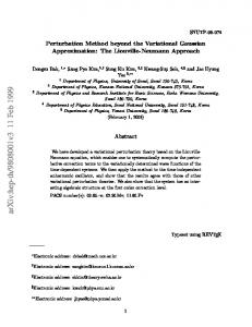
rates chosen adaptively according to the ADADELTA approach (Zeiler, 2012). We use the gradient estimators in Roeder et al. (2017), i.e. (16), (18), (21) and (23), although we found no noticeable difference compared to (15), (17), (20) and (22), which is likely due to the small number of factors as described in Sections 2 and 4. Our choice was motivated by computational efficiency as some terms cancel out using the approach in Roeder et al. (2017). We initialize B and C as unit diagonals and, for parity, µ and D are chosen to match the starting values of the Gibbs sampler in Wikle and Hooten (2006). Figure 1 monitors the convergence via the estimated value of L(λ) using a single Monte Carlo sample. Table 1 presents estimates of L(λ) at the final iteration using 100 Monte Carlo samples. The results suggest that the best VB parametrization in terms of ELBO is the lowrank state algorithm (LR-SA) with, importantly, a high-dimensional state-mean (HD-SM) (otherwise the poorest VB approximation is achieved, see Table 1). However, Table S1 shows that this parametrization is about three times as CPU intensive. The fastest VB parametrizations are both Low-Rank State (LR-S) algorithms, and modeling the state mean separately for these does not seem to improve L(λ) (Table 1) and is also slightly more computationally expensive (Table S1). Taking these considerations into account, the final choice of VB parametrization we use for this model is the low-rank state with low-dimensional state mean (LR-S + LD-SM). We show in Section 5.5 that this parametrization gives accurate approximations for our analysis. For the rest of this example we benchmark the VB posterior from
−10000 −15000 −20000
LR−S + LD−SM LR−S + HD−SM LR−SA + LD−SM LR−SA + HD−SM
−30000
−25000
Evidence lower bound
−5000
0
LR-S + LD-SM against the MCMC approach in Wikle and Hooten (2006).
0
2000
4000
6000
8000
10000
Iteration
Figure 1: L(λ) for the variational approximations for the spatio-temporal example. The figure shows the estimated value of L(λ) vs iteration number for the four different parametrizations, see Section 5.3 or Table 1 for abbreviations.
18
Table 1: L(λ) and CPU time for the VB parametrizations in the spatio-temporal and Wishart process example. The table shows the estimated value of L(λ) for the different VB parametrizations by combining low-rank state / low-rank state and auxiliary (LR-S / LR-SA) with either of low-dimensional state mean / highdimensional state mean (LD-SM / HD-SM). The estimate and its 95% confidence interval are computed at the final iteration using 100 Monte Carlo samples. The figure also show the relative CPU (R-CPU) time, where the reference is LD-SM. Parametrization Spatio-temporal
R-CPU
L(λopt )
Confidence interval
LR-S + LD-SM
1
−1, 996
[−2, 004; −1, 988]
LR-S + HD-SM
1.005
−2, 024
[−2, 032; −2, 016]
LR-SA + LD-SM
3.189
−2, 158
[−2, 167; −2, 148]
LR-SA + HD-SM
3.017
−1, 909
[−1, 918; −1, 900]
LR-S + LD-SM
1
−1, 588
[−1, 593; −1, 583]
LR-S + HD-SM
1.0004
−1, 501
[−1, 506; −1, 495]
Wishart process
5.4
Settings for MCMC
Before evaluating VB against MCMC, we need to determine a reasonable burn-in and number of iterations for the Gibbs sampler in Wikle and Hooten (2006). It is clear that it is not feasible to monitor convergence for every single parameter in such a large scale model as (24), and therefore we focus on ψ, u18 and v19 , which are among the variables considered in the analysis in Section 5.5. Wikle and Hooten (2006) use 50, 000 iterations of which 20, 000 are discarded as burnin. We generate 4 sampling chains with these settings and inspect convergence using the coda package (Plummer et al., 2006) in R. We compute the Scale Reduction Factors (SRF) (Gelman and Rubin, 1992) for ψ, u18 and v19 as a function of the number of Gibbs iterations. The adequate number of iterations in MCMC depends on what functionals of the parameters are of interest; here we monitor convergence for these quantities since we report marginal posterior distributions for these quantities later. The scale reduction factor of a parameter measures if there is a significant difference between the variance within the four chains and the
19
variance between the four chains of that parameter. We use the rule of thumb that concludes convergence when SRF < 1.1, which gives a burn-in period of approximately 40, 000 here, for these functionals. After discarding these samples and applying a thinning of 10 we are left with 1, 000 posterior samples for inference. However, as the draws are auto-correlated, this does not correspond to 1, 000 independent draws used in the analysis in Section 5.5 (note that we obtain independent samples from our variational posterior). To decide how many Gibbs samples are equivalent to 1, 000 independent samples for ψ, u18 and v19 , we compute the Effective Sample Size (ESS) which takes into account the auto-correlation of the samples. We find that the smallest is ESS = 5 and hence we require 200, 000 iterations after a thinning of 10, which makes a total of 2, 000, 000 Gibbs iterations, excluding the burn-in of 40, 000. Thinning is advisable here due to memory issues.
5.5
Analysis and results
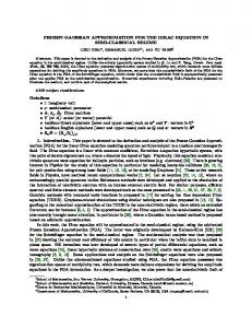
We first consider inference on the diffusion coefficient ψi for location i. Figure 2 shows the “true” posterior (represented by MCMC) together with the variational approximation for six locations described in the caption of the figure. The figure shows that the posterior distribution is highly skewed for locations with zero dove counts and approaches normality as the dove counts increase. Consequently, the accuracy of the variational posterior (which is Gaussian) improves with increasing dove counts.
20
Location i = 96
Location i = 35
Location i = 1 Algorithm Density of ψi
MCMC VB
−0.2
0.0
0.2
0.4
−0.2
0.0
0.2
0.4
−0.2
Location i = 46
0.2
0.4
Location i = 105
Density of ψi
Location i = 5
0.0
−0.2
0.0
0.2
0.4
−0.2
0.0
0.2
0.4
0.6
−0.2 −0.1
0.0
0.1
0.2
0.3
Figure 2: Distribution of the diffusion coefficients. The figure shows the posterior distribution of ψi obtained by MCMC and VB. The locations are divided into three categories (total doves over time within brackets): zero count locations (Idaho, i = 1 [0] , Arizona i = 5 [0], left panels), low count locations (Texas, i = 35 [16], 46 [21], middle panels) and high count locations (Florida, i = 96 [1, 566], 105 [1, 453], right panels). Draws from VB posterior of ϕt
Draws from MCMC posterior of ϕt 1200
1200
1000
1000
800
800
ϕt
1400
ϕt
1400
400
200
200
0
0 1986 1987 1988 1989 1990 1991 1992 1993 1994 1995 1996 1997 1998 1999 2000 2001 2002 2003
600
400
1986 1987 1988 1989 1990 1991 1992 1993 1994 1995 1996 1997 1998 1999 2000 2001 2002 2003
600
Year t
Year t
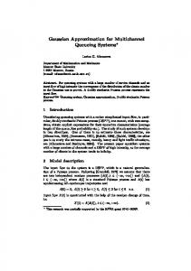
Figure 3: Samples from the posterior sum of dove intensity over the spatial grid for each year. The figure shows 100 samples from the posterior distribution of P ϕt = i exp(vit ) obtained by MCMC (left panel) and VB (right panel). Figure 3 shows 100 VB and MCMC posterior samples of the dove intensity for each year P summed over the spatial locations, i.e. ϕt = i exp(vit ). Both posteriors are very similar and, in particular, show an exponential increase of doves until year 2002 followed by a steep decline for year 2003. In the interest of analyzing the spatial dimension of the model, Figure 4 shows a heat map of the MCMC and VB posterior mean of the dove intensity ϕit = exp(vit ) for the last five years of the data, overlaid on a map of the United States of America. We draw the 21
following conclusions from the analysis using the MCMC and VB posteriors (which are nearly identical). First, the dove intensity is most pronounced in the South East states, in particular Florida (Figure 4). Second, the decline of doves for year 2003 in Figure 3 is likely attributed to a drop in the intensity (Figure 4) at two areas of Florida: Central Florida (i = 96) and South East Florida (i = 105). Figure 5 illustrates the whole posterior distribution of the logintensity for these locations at year 2003 and, moreover, an out-of-sample posterior predictive distribution for year 2004. The estimates are obtained by kernel density estimates using approximately 1, 000 effective samples. The posterior distributions for the VB and MCMC are similar, and it is evident that using this large scale model for forecasting future values is
maplocs_extend
associated with a large uncertainty.
maplocs_extend maplocs_extend
maplocs[, 1]
maplocs_extend
1999 maplocs[, 1]
maplocs[, 1]
2002
2002
maplocs[, 1]
maplocs_extend
1999 maplocs[, 1]
maplocs[, 1]
2000
2000
maplocs[, 1]
2001
2001
maplocs[, 1]
2003
2003
Figure 4: Posterior dove intensity for the years 1999-2003. The figure shows the posterior mean of ϕit = exp(vit ) computed by MCMC (left panels) and VB (right panels) for i = 1, . . . , p = 111, and the last 5 years of the data (t = 14, 15, 16, 17, 18). The results are illustrated with a spatial grid plotted together with a map of the United States, where the colors vary between low intensity (yellow) and high intensity (red). The light blue color is for aesthetic reasons and does not correspond to observed locations. We conclude this example by investigating the spatial functions and their reweighting over 22
time to produce the variational approximation. Figure 6 illustrates this and shows that the correlation among the states is mostly driven by spatial locations outside the southern east part of North America. This is reasonable as the data contains mostly zero or near zero counts outside the southern east region. Location i = 105
Density of vt = log(ϕt) at year 2003 (t=18)
Location i = 96
Algorithm
MCMC VB
5.2
5.4
4.25
4.50
4.75
Density of vt = log(ϕt) at year 2004 (t=19)
5.0
−10
0
10
20
−10
0
10
20
Figure 5: Forecasting the log intensity of the spatial process. The figure shows an in-sample forecast of the log-intensity vit for year 2003 (t = 18, upper panels) and out-of-sample forecast for year 2004 (t = 19, lower panels) for Central Florida (i = 96, left panels) and South East Florida (i = 105, right panels). The analysis in this section shows that similar inferential conclusions are drawn with the VB posterior and the “true” posterior (approximated by the Gibbs sampler). One advantage with the VB posterior is that it is more efficient for performing posterior predictive analysis because independent samples are easily obtained, in contrast to MCMC samples that may have a prohibitively large auto-correlation, resulting in imprecise estimators. Perhaps the main advantage of the VB posterior is that it is faster to obtain: in this particular application VB was 7.3 times faster than MCMC. The speed up in computing time relative to MCMC is model specific and depends on how expensive the different sampling steps in the Gibbs sampler are. This spatial temporal model is computationally cheap on a per iteration basis, however, many iterations are needed for accurate inference as demonstrated. In the next section, we consider a model which is both computationally expensive and mixes poorly. For that model the computational gains are much more pronounced. 23
Weight of spatial basis 1 t(weights_basis)
Spatial basis 1
Spatial basis 2
Weight of spatial basis 2 t(matrix(rep(0:18, 4), ncol = 4))
t(weights_basis)
1 3
Spatial basis 3
Weight of spatial basis 3 t(matrix(rep(0:18, 4), ncol = 4))
t(weights_basis)
1 3
Spatial basis 4
Weight of spatial basis 4 t(matrix(rep(0:18, 4), ncol = 4))
t(weights_basis)
1 3
Figure 6: Spatial basis representation of the state vector. The figure shows the Spatial basis functions (left panel), i.e. the jth column of B, j = 1, . . . , q = 4 and the corresponding weights µt (right panel) through t = 0, . . . , 18, that forms E(Xt ) = Bµt .
6
Application 2: Stochastic volatility modeling
6.1
Industry portfolios data
Our second example considers the Multivariate stochastic volatility model via Wishart processes in Philipov and Glickman (2006b) used for modeling the time-varying dependence of a portfolio of k assets over T time periods. We follow Philipov and Glickman (2006b) and use k = 5 (manufacturing, utilities, retail/wholesale, finance, other) which results in a state-vector (the lower-triangular part of the covariance matrix) of dimension p = 15. This is far from a high-dimensional setting, but allows us to implement an MCMC method to compare against the variational approximation. In fact, for k = 12, which gives p = 78, Philipov and Glickman (2006b) use a Metropolis-Hastings within Gibbs sampler and reported that some of the blocks updated by the Metropolis-Hastings sampler have acceptance probabilities close to zero. We discuss this further in Section 6.4 and note at the outset that our variational approach does not have this limitation as we demonstrate in Section 6.5. Philipov and Glickman (2006b) made a mistake in the derivation of the Gibbs sampler which affects all full conditionals (Rinnergschwentner et al., 2012). Implementing the corrected 24
version results in a highly inefficient sampler and we take T = 100 instead of T = 240 so that the MCMC can finish in a reasonable amount of time. Hence we have T = 100 montly observations on value-weighted portfolios from the 201709 CRSP database, covering a period from 2009-06 to 2017-09. We follow Philipov and Glickman (2006b) and prefilter each series using an AR(1) process.
6.2
Model
We assume that the return at time period t, t = 1, . . . , T , is the vector yt = (yt1 , . . . , ytk )> , yt ∼ N (0, Σt ),
Σt ∈ Rp×p
1 d > p×p , ν > k, 0 < d < 1, H(Σ−1 t ) H , St ∈ R ν H is a lower triangular Cholesky factor of a positive definite matrix A, A = HH > ∈ Rp×p and ∼ Wishart(ν, St−1 ), Σ−1 t
St =
Σ0 is assumed known. Philipov and Glickman (2006b) use an inverse Wishart prior for A, A−1 ∼ Wishart(γ0 , Q0 ), γ0 = k + 1, Q0 = I, a uniform prior for d, d ∼ U [0, 1], and a shifted gamma prior for ν, ν − k ∼ Gamma(α0 , β0 ). The joint posterior density for (Σ, A, ν − k, d) is p(Σ, A, ν − k, d|y) ∝ p(A, d, ν − k)
T Y
p(Σt |ν, St−1 )p(yt |Σt ),
(25)
t=1
where p(A, d, ν − k) denotes the joint prior density for (A, d, ν − k), p(Σt |ν, St−1 , d) denotes the conditional inverse Wishart prior for Σt given ν, St−1 and d, and p(yt |Σt ) is the normal density for yt given Σt . We reparametrize the posterior in terms of the unconstrained parameter θ = (vech(H 0 )> , d0 , ν 0 , vech(C10 )> , . . . , vech(CT0 )> )> , where Ct0 ∈ Rk×k ,
0 0 Ct,ij = Ct,ij , i 6= j, and Ct,ii = log Ct,ii ,
H 0 ∈ Rk×k ,
Hij0 = Hij , i 6= j, and Hii = log Hii,
and d0 = log d/(1 − d), and ν 0 = log(ν − k). Then, as shown in Section S1.3, (T ) Y > > |Lk (Ik2 + Kk,k )(Ct ⊗ Ik )Lk | × (ν − k) p(θ|y) ∝|Lk (Ik2 + Kk,k )(H ⊗ Ik )Lk |× × d(1 − d) ×
( Y i
Hii
t=1 )( T k YY
)
Ct,ii
t=1 i=1
× p(A, d, ν − k)
(T Y
(26) )
p(Σt |ν, St−1 , d)p(yt |Σt ) ,
t=1
where Lk denotes the elimination matrix, which for a k × k matrix A satisfies vech(A) = Lk vec(A), and as before K is the commutation matrix. Evaluation of the gradient of the log posterior is described in the Section S1.4. 25
6.3
Variational approximations of the posterior distribution
Since this example does not include a high-dimensional auxiliary variable, we use the low-rank state (LR-S) parametrization combined with both a low-dimensional state mean (LD-SM) and a high-dimensional state mean (HD-SM). As in the previous example, it is straightforward to deduce conditional independence relationships in (26) to build the Cholesky factor C2 of the precision matrix Ω2 of ζ in Section 4. Moreover, construction of the Cholesky factor C1 of the precision matrix Ω1 of z is outlined in Section 4. Massive parsimony is achieved in this application, in particular for k = 12 assets in which the saturated Gaussian variational approximation has 31, 059, 020 parameters, while our parametrization gives 10, 813. For k = 5, the saturated case has 1, 152, 920 parameters and our parametrizations give 4, 009-5, 109; see Section S3 for more details. For all variational approximations we let q = 4 and run 10, 000 iterations of a stochastic optimization algorithm with learning rates chosen adaptively according to the ADADELTA approach (Zeiler, 2012). We initialize B and C as unit diagonals and choose µ and D randomly. Figure 7 monitors the estimated ELBO for both parametrizations, using both the gradient estimators in Roeder et al. (2017) and the alternative standard ones which do not cancel terms that have zero expectation. For k = 5, the figure shows that the different gradient estimators perform equally well. Moreover, slightly more variable estimates are observed in the beginning for the low-dimensional state mean parametrization compared to that of the high-dimensional mean. Table 1 presents estimates of L(λ) at the final iteration using 100 Monte Carlo samples and also presents the relative CPU times of the algorithms. In this example the separate state mean present in the high-dimensional state mean seems to improve the ELBO considerably.
0
2000
6000
10000
Stochastic VB iteration
2000
6000
10000
Stochastic VB iteration
−5000 −20000
Evidence lower bound 0
LD−SM for k = 12
−35000
−4000 −8000
Standard Roeder et al.
−12000
−8000
−4000
Evidence lower bound
HD−SM for k = 5
−12000
Evidence lower bound
LD−SM for k = 5
0
2000
6000
10000
Stochastic VB iteration
Figure 7: L(λ) for the variational approximations in the Wishart process example. The figure shows the estimated value of L(λ) vs iteration number using a lowdimensional state mean / high-dimensional state mean (LD-SM / HD-SM) with the gradient estimator in Roeder et al. (2017) or the standard estimator. The results are shown for k = 5 (left and middle panel) and k = 12 (right panel).
26
6.4
Settings for MCMC
While we can do a thorough analysis to determine the burn-in and number of iterations for the Gibbs sampler in Wikle and Hooten (2006), this task becomes much more complicated here for the following reasons. First, Philipov and Glickman (2006b) use the inverse cdf method on a grid to sample ν and d, which increases the computational burden compared to Wikle and Hooten (2006). Second, due to an erroneous step in the derivation of the full conditional of A−1 (Rinnergschwentner et al., 2012), it cannot be directly sampled from a Wishart distribution as in Philipov and Glickman (2006b). We instead implement a random-walk MetropolisHastings update for A−1 with a mean equal to the current value in the MCMC. Third, the erroneous step results in changes for all the full conditionals. The latter two reasons might explain why we do not observe the same sampling efficiency as Philipov and Glickman (2006b). Consequently, we obtain poor values for the effective sample size and therefore, if combined with the first reason explained above, we would have to wait for several months to obtain an effective sample size of 1, 000 as in our previous example, even when reducing T = 240 to T = 100 as explained in Section 6.1. We conclude that this application is very difficult for our Metropolis-Hastings within Gibbs sampler when k = 5 (and impossible for k = 12) and settle for 100, 000 iterations and discard 20, 000 for burn-in, which arguably are numbers many practitioners would think are sufficient. After thinning the draws, we obtain 1, 000 posterior samples and the effective sample sizes are 10 for d, 78 for ν, 45 (average) for A and 503 (average) for Σ. Note the low values for d, ν and A, whose chains exhibit a very persistent behavior (not shown here), whereas the effective sample size is higher for Σ (because of the independent proposal). We stress that because MCMC convergence is questionable (in particular for d, ν and A), so is the MCMC posterior produced and we cannot, unfortunately, know if discrepancies between the methods is due to a poor variational approximation or a poorly estimated MCMC posterior. Nevertheless, the VB posterior seems to give a reasonable predictive distribution for the data and is therefore considered to produce sensible results. The main reasons that the sampler in Philipov and Glickman (2006b) fails when k = 12 is due to an independent Wishart proposal within Gibbs for t < T (at t = T perfect sampling from a Wishart can be applied) and for updating Σ−1 t the random-walk proposal within Gibbs for A−1 . It is well-known that these proposals fail in a high-dimensional setting: the random-walk explores the sampling space extremely slowly while independent samplers get stuck, i.e. reject nearly all attempts to move the Markov chain. We remark that other MCMC approaches for estimating this model more efficiently might be possible, but it is outside the scope of this paper to pursue this. As an example, Hamiltonian 27
Monte Carlo on the Riemannian manifold (Girolami and Calderhead, 2011) has proven to be effective in sampling models with 500-1, 000 parameters. However, the computational burden relative to standard MCMC is increased and, moreover, tuning the algorithm becomes more difficult.
6.5
Analysis and results
Section 5 considered a thorough example on how the variational posterior can be used to conduct a wide range of inferential tasks in a serious application. For brevity, we now only study the accuracy of the variational posterior compared to that of MCMC (although we need to be skeptical about the MCMC posterior as explained in Section 6.4) and also check if the predictive distribution gives reasonable results. Figure 8 shows kernel density estimates of the MCMC and VB posterior of the distinct elements of A, ν and d based on 1, 000 samples. The marginal posteriors are very similar for some parameters of A (for example A15 , A25 and A35 ) but not for others (for example A11 , A33 and A55 ). For ν and δ the difference is considerable, but recall that MCMC convergence is questionable. To assess the approximation of Σt , t = 1, . . . , T , we inspect the in-sample predictive distribution for the data, i.e p(˜ yt |y1:T ) for t = 1, . . . , T, obtained by averaging over the posterior of Σt using simulation. Figure 9 shows the results together with the observed data, which confirms that both estimation approaches yield predictions consistent with the data. We argued that our variational approximation can handle very large dimensions in this model and discussed that MCMC fails, see Section 6.4. Indeed, Figure 7 also shows the estimated ELBO on a variational optimization using all assets, which corresponds to k = 12 with p = 78. While it is more variable than the k = 5 case, it settles down eventually. At the last iteration, we use the variational approximation (which has a low-dimensional state mean) and compute the predictive distribution and compare it do the data to ensure the results are sensible (not shown here). Note that we choose to use the low-dimensional state-mean here since we know that the richer model high-dimensional state provides a better approximation. The speed up for VB vs MCMC when k = 5 was 29 times in this application, which is likely a very loose lower bound because the convergence of MCMC is questionable as discussed in Section 6.4. For k = 12, we demonstrate that the variational optimization converges and hence the variational approximation allows for inference, as opposed to MCMC which, in practice, does not produce a single effective draw due to the poor mixing.
28
−0.2
0.0
−0.2 −0.1 0.0
−1.0
−0.8
0.1
−0.6
0.2
0.2
−0.4
−0.3 −0.2 −0.1 0.0
−0.1
0.0
0.1
Dens of A35
0.5
0.1
0.2
Dens of A44
0.4
Dens of A45
Dens of A23
0.2
0.3
0.2
−0.6
−0.4
0.2
0.3
−0.6
−0.4 −0.3 −0.2 −0.1 0.0
0.4
−0.2
0.5
−0.4
Dens of A55
0.0
0.2
0.0
0.6
−0.2
1.0
1.5
Dens of ν
−0.4
1.2
Dens of A24
−0.2
0.9
Dens of A25
0.6
Dens of A33
0.3
Dens of A34
Dens of A15
Dens of A14
Dens of A13
Dens of A12
Dens of A11
MCMC VB
0.4
0.6
0.8
1.0
10
30
50
Dens of d
Dens of A22
Algorithm
−0.2 −0.1 0.0
0.1
0.2
0.3
0.0
0.2
0.4
0.6
Figure 8: Kernel density estimates for A, ν and d. The figure shows the posterior distribution of A, ν and d obtained by MCMC and VB.
7
Discussion
We have considered an approach to Gaussian variational approximation for high-dimensional state space models where dimension reduction in the variational approximation is achieved through a dynamic factor structure for the variational covariance matrix. The factor structure reduces the dimension in the description of the states, whereas the Markov dynamic structure for the factors achieves parsimony in describing the temporal dependence. We have shown that the method works well in two challenging models. The first is an extended example for a spatio-temporal data set describing the spread of the Eurasian collared-dove throughout North America. The second is a multivariate stochastic volatility model in which the statevector, which is the half vectorization of the Cholesky factor of the covariance matrix, is high-dimensional. Perhaps the most obvious limitation of our current work is the restriction to a Gaussian approximation, which does not allow capturing skewness or heavy tails in the posterior distribution. However, Gaussian variational approximations can be used as building blocks for more complex approximations based on normal mixtures or copulas for example (Han et al., 2016; Miller et al., 2016) and these more complex variational families can overcome some of
29
Manufacturing 20
Utilities
Retail / Wholesale
20
VB MCMC
20
●
−10
10
●
● ● ● ● ●● ● ●● ● ● ● ● ● ●● ● ● ● ● ● ● ● ● ●●● ● ● ● ●● ● ●● ● ●● ●● ●● ●● ● ● ● ●● ● ● ● ● ● ● ● ● ●● ● ● ● ●● ● ●● ●● ● ● ● ● ●● ● ● ● ● ● ● ● ● ● ● ● ● ● ● ● ● ● ● ● ● ●
10 ●● ● ● ● ● ● ● ●● ● ● ● ●●● ● ● ● ● ●● ● ● ● ● ● ●● ● ● ● ●● ● ●● ● ● ●● ● ● ● ●● ●● ●● ● ● ● ● ●● ● ● ● ● ● ● ● ● ● ● ● ● ●● ● ● ● ● ● ●● ● ● ● ● ● ● ● ● ● ● ●● ● ● ● ● ● ●
● ●
0
● ●
●
~ y t3
0
●
~ y t2
~ y t1
10
0
−10
−10
−20
−20
● ● ● ● ● ● ● ● ●● ● ●● ● ●● ●●● ● ● ●● ● ● ● ● ●● ● ●● ● ● ●● ●● ● ● ● ●● ● ●● ● ● ● ● ●● ● ●● ●● ● ●● ● ● ● ● ● ● ● ●● ● ● ● ●● ●● ● ● ●● ● ● ● ● ●● ● ●● ● ● ● ● ● ● ● ● ● ● ●
2009−06 2010−03 2011−01 2011−11 2012−09 2013−07 2014−05 2015−03 2016−01 2016−11 2017−09
2009−06 2010−03 2011−01 2011−11 2012−09 2013−07 2014−05 2015−03 2016−01 2016−11 2017−09
−20
Finance
Other
20
20
● ●
0
−10
●
10
● ● ●
● ● ● ● ● ● ●● ● ● ● ● ● ● ● ●● ●●● ●● ● ● ● ●●● ● ● ●● ● ● ● ● ● ● ● ● ● ● ● ● ●● ● ●● ● ● ● ● ● ● ● ●● ● ●● ● ● ● ● ● ● ●●● ● ● ●● ●● ● ● ● ● ● ● ● ● ● ● ● ● ● ● ● ● ● ● ● ● ● ●
● ● ●
● ● ●●
● ●
●
● ● ● ● ●● ●● ●● ● ●● ● ●● ● ●●● ● ● ●● ●● ● ● ●● ● ● ● ● ● ● ●● ●● ● ● ● ● ● ● ● ● ● ● ● ● ● ●● ● ● ● ● ● ●●● ● ●●● ● ● ●● ● ● ● ● ●● ● ● ● ● ●
−10
●
●
−20 2009−06 2010−03 2011−01 2011−11 2012−09 2013−07 2014−05 2015−03 2016−01 2016−11 2017−09
−20
0
2009−06 2010−03 2011−01 2011−11 2012−09 2013−07 2014−05 2015−03 2016−01 2016−11 2017−09
~ y t4
● ●
~ y t5
10
2009−06 2010−03 2011−01 2011−11 2012−09 2013−07 2014−05 2015−03 2016−01 2016−11 2017−09
●
Figure 9: Posterior predictive distribution of the data. The figure shows the posterior predictive distribution together with the data (black circles) for each time period obtained by MCMC and VB for the different portfolios. the limitations of the simple Gaussian approximation. We intend to consider this in future work.
Acknowledgements We thank Mevin Hooten for his help with the Eurasian collared-dove data. We thank Linda Tan for her comments on an early version of this manuscript. Matias Quiroz and Robert Kohn were partially supported by Australian Research Council Center of Excellence grant CE140100049. David Nott was supported by a Singapore Ministry of Education Academic Research Fund Tier 2 grant (MOE2016-T2-2-135).
References Aguilar, O. and West, M. (2000). Bayesian dynamic factor models and portfolio allocation. Journal of Business & Economic Statistics, 18(3):338–357.
30
Andrieu, C., Doucet, A., and Holenstein, R. (2010). Particle Markov chain Monte Carlo methods. Journal of the Royal Statistical Society, Series B, 72:1–33. Andrieu, C. and Roberts, G. (2009). The pseudo-marginal approach for efficient Monte Carlo computations. The Annals of Statistics, 37:697–725. Archer, E., Park, I. M., Buesing, L., Cunningham, J., and Paninski, L. (2016). Black box variational inference for state space models. arXiv:1511.07367. Attias, H. (1999). Inferring parameters and structure of latent variable models by variational Bayes. In Laskey, K. and Prade, H., editors, Proceedings of the 15th Conference on Uncertainty in Artificial Intelligence, pages 21–30. Morgan Kaufmann. Barber, D. and Bishop, C. M. (1998). Ensemble learning for multi-layer networks. In Jordan, M. I., Kearns, M. J., and Solla, S. A., editors, Advances in Neural Information Processing Systems 10, pages 395–401. MIT Press. Bartholomew, D. J., Knott, M., and Moustaki, I. (2011). Latent variable models and factor analysis: A unified approach, 3rd edition. John Wiley & Sons. Beaumont, M. A. (2003). Estimation of population growth or decline in genetically monitored populations. Genetics, 164:1139–1160. Blei, D. M., Kucukelbir, A., and McAuliffe, J. D. (2017). Variational inference: A review for statisticians. Journal of the American Statistical Association, 112(518):859–877. Bottou, L. (2010). Large-scale machine learning with stochastic gradient descent. In Lechevallier, Y. and Saporta, G., editors, Proceedings of the 19th International Conference on Computational Statistics (COMPSTAT’2010), pages 177–187. Springer. Carlin, B. P., Polson, N. G., and Stoffer, D. S. (1992). A Monte Carlo approach to nonnormal and nonlinear state-space modeling. Journal of the American Statistical Association, 87(418):493–500. Carter, C. K. and Kohn, R. (1994). On Gibbs sampling for state space models. Biometrika, 81(3):541–553. Carvalho, C. M., Chang, J., Lucas, J. E., Nevins, J. R., Wang, Q., and West, M. (2008). Highdimensional sparse factor modeling: Applications in gene expression genomics. Journal of the American Statistical Association, 103(484):1438–1456.
31
Caswell, H. and van Daalen, S. F. (2016). A note on the vec operator applied to unbalanced block-structured matrices. Journal of Applied Mathematics, 2016. Article ID 4590817. Challis, E. and Barber, D. (2013). Gaussian Kullback-Leibler approximate inference. Journal of Machine Learning Research, 14:2239–2286. Cressie, N. and Wikle, C. (2011). Statistics for Spatio-Temporal Data. Wiley. Doucet, A., Pitt, M. K., Deligiannidis, G., and Kohn, R. (2015). Efficient implementation of Markov chain Monte Carlo when using an unbiased likelihood estimator. Biometrika, 102:295–313. Gelman, A. and Rubin, D. B. (1992). Inference from iterative simulation using multiple sequences. Statistical Science, pages 457–472. Geweke, J. and Zhou, G. (1996). Measuring the pricing error of the arbitrage pricing theory. Review of Financial Studies, 9(2):557–587. Girolami, M. and Calderhead, B. (2011). Riemann manifold Langevin and Hamiltonian Monte Carlo methods. Journal of the Royal Statistical Society: Series B (Statistical Methodology), 73(2):123–214. Han, S., Liao, X., Dunson, D. B., and Carin, L. C. (2016). Variational Gaussian copula inference. In Gretton, A. and Robert, C. C., editors, Proceedings of the 19th International Conference on Artificial Intelligence and Statistics, volume 51, pages 829–838, Cadiz, Spain. JMLR Workshop and Conference Proceedings. Hoffman, M. D., Blei, D. M., Wang, C., and Paisley, J. (2013). Stochastic variational inference. Journal of Machine Learning Research, 14:1303–1347. Ji, C., Shen, H., and West, M. (2010). Bounded approximations for marginal likelihoods. Technical Report 10-05, Institute of Decision Sciences, Duke University. Jordan, M. I., Ghahramani, Z., Jaakkola, T. S., and Saul, L. K. (1999). An introduction to variational methods for graphical models. Machine Learning, 37:183–233. Kingma, D. P. and Welling, M. (2014). Auto-encoding variational Bayes. In Proceedings of the 2nd International Conference on Learning Representations (ICLR) 2014. https: //arxiv.org/abs/1312.6114.
32
Krishnan, R. G., Shalit, U., and Sontag, D. (2017). Structured inference networks for nonlinear state space models. In Proceedings of the Thirty-First AAAI Conference on Artificial Intelligence, February 4-9, 2017, San Francisco, California, USA., pages 2101–2109. Ku, Y.-C., Bloomfield, P., and Ghosh, S. K. (2014). A flexible observed factor model with separate dynamics for the factor volatilities and their correlation matrix. Statistical Modelling, 14(1):1–20. Kucukelbir, A., Tran, D., Ranganath, R., Gelman, A., and Blei, D. M. (2017). Automatic differentiation variational inference. Journal of Machine Learning Research, 18(14):1–45. Lopes, H. F., Salazar, E., and Gamerman, D. (2008). Spatial dynamic factor analysis. Bayesian Analysis, 3(4):759–792. Magnus, J. R. (1985). On differentiating eigenvalues and eigenvectors. Econometric Theory, 1:179–191. Magnus, J. R. and Neudecker, H. (1985). Matrix differential calculus with applications to simple, Hadamard, and Kronecker products. Journal of Mathematical Psychology, 29:474– 492. Miller, A. C., Foti, N., and Adams, R. P. (2016). Variational boosting: Iteratively refining posterior approximations. arXiv: 1611.06585. Nott, D. J., Tan, S. L., Villani, M., and Kohn, R. (2012). Regression density estimation with variational methods and stochastic approximation. Journal of Computational and Graphical Statistics, 21:797–820. Ong, V. M.-H., Nott, D. J., and Smith, M. (2017). Gaussian variational approximation with factor covariance structure. arXiv:1701.03208. Opper, M. and Archambeau, C. (2009). The variational Gaussian approximation revisited. Neural Computation, 21:786–792. Ormerod, J. T. and Wand, M. P. (2010). Explaining variational approximations. The American Statistician, 64:140–153. Paisley, J. W., Blei, D. M., and Jordan, M. I. (2012). Variational Bayesian inference with stochastic search. In Langford, J. and Pineau, J., editors, Proceedings of the 29th International Conference on Machine Learning, ICML 2012. http://icml.cc/2012/papers/ 687.pdf. 33
Philipov, A. and Glickman, M. E. (2006a). Factor multivariate stochastic volatility via Wishart processes. Econometric Reviews, 25(2-3):311–334. Philipov, A. and Glickman, M. E. (2006b). Multivariate stochastic volatility via Wishart processes. Journal of Business & Economic Statistics, 24(3):313–328. Pitt, M. K., dos Santos Silva, R., Giordani, P., and Kohn, R. (2012). On some properties of Markov chain Monte Carlo simulation methods based on the particle filter. Journal of Econometrics, 171(2):134–151. Plummer, M., Best, N., Cowles, K., and Vines, K. (2006). CODA: convergence diagnosis and output analysis for MCMC. R News, 6(1):7–11. Ranganath, R., Gerrish, S., and Blei, D. M. (2014). Black box variational inference. In Kaski, S. and Corander, J., editors, Proceedings of the 17th International Conference on Artificial Intelligence and Statistics, volume 33, pages 814–822. JMLR Workshop and Conference Proceedings. Rezende, D. J., Mohamed, S., and Wierstra, D. (2014). Stochastic backpropagation and approximate inference in deep generative models. In Xing, E. P. and Jebara, T., editors, Proceedings of the 29th International Conference on Machine Learning, ICML 2014. proceedings.mlr.press/v32/rezende14.pdf. Rinnergschwentner, W., Tappeiner, G., and Walde, J. (2012). Multivariate stochastic volatility via Wishart processes: A comment. Journal of Business & Economic Statistics, 30(1):164– 164. Robbins, H. and Monro, S. (1951). A stochastic approximation method. The Annals of Mathematical Statistics, 22:400–407. Roeder, G., Wu, Y., and Duvenaud, D. (2017). Sticking the landing: Simple, lower-variance gradient estimators for variational inference. arXiv preprint arXiv:1703.09194. Salimans, T. and Knowles, D. A. (2013). Fixed-form variational posterior approximation through stochastic linear regression. Bayesian Analysis, 8:837–882. Seeger, M. (2000). Bayesian model selection for support vector machines, Gaussian processes and other kernel classifiers. In Solla, S. A., Leen, T. K., and M¨ uller, K., editors, Advances in Neural Information Processing Systems 12, pages 603–609. MIT Press.
34
Tan, L. S. and Nott, D. J. (2017). Gaussian variational approximation with sparse precision matrices. Statistics and Computing, pages 1–17. Titsias, M. and L´azaro-Gredilla, M. (2014). Doubly stochastic variational Bayes for nonconjugate inference. In Xing, E. P. and Jebara, T., editors, Proceedings of the 29th International Conference on Machine Learning, ICML 2014. proceedings.mlr.press/v32/ titsias14.pdf. Titsias, M. and L´azaro-Gredilla, M. (2015). Local expectation gradients for black box variational inference. In Cortes, C., Lawrence, N., Lee, D., Sugiyama, M., and Garnett, R., editors, Advances in Neural Information Processing Systems 28 (NIPS 2015), pages 2638– 2646. Curran Associates, Inc. Wikle, C. and Cressie, N. (1999). A dimension-reduced approach to space-time Kalman filtering. Biometrika, 86(4):815–829. Wikle, C. K. and Hooten, M. B. (2006). Hierarchical Bayesian spatio-temporal models for population spread. In Clark, J. S. and Gelfand, A., editors, Applications of computational statistics in the environmental sciences: hierarchical Bayes and MCMC methods, pages 145–169. Oxford University Press: Oxford. Winn, J. and Bishop, C. M. (2005). Variational message passing. Journal of Machine Learning Research, 6:661–694. Woodbury, M. A. (1950). Inverting modified matrices. Memorandum report, 42(106):336. Zeiler, M. D. (2012). ADADELTA: An adaptive learning rate method. arXiv: 1212.5701.
35
Supplement to ‘Gaussian variational approximation for high-dimensional state-space models’. We refer to equations, sections, etc in the main paper as (1), Section 1, etc, and in the supplement as (S1), Section S1, etc.
S1 S1.1
Derivations Gradients of the variational approximation
This section derives the gradient expressions stated in Section 4. The following result about the vec and Kronecker product is useful. For conformably dimensioned matrices A, B and C, vec(ABC) = (C > ⊗ A)vec(B). First, note that if θ ∼ qλ (θ), then we have θ = W µ + W C −> ω + Ze (where the notation is the same as in Section 4) and p(T + 1) + P 1 log 2π − log|W ΣW > + Z 2 | 2 2 1 −> > − (W C ω + Ze) (W ΣW > + Z 2 )−1 (W C −> ω + Ze). 2
log qλ (θ) = −
(S1)
Since the above does not depend on µ, ∇µ L(λ) =∇µ Ef (log h(W µ + W C −> ω + Ze)) =Ef (W > ∇θ log h(W µ + W C −> ω + Ze)). Next, consider ∇vec(B) L(λ). For the parametrization outlined in Section 3.3, we use the derivation in Ong et al. (2017), � � 1 > 2 ∇vec(B) Ef log|BB + D | =vec((BB > + D2 )−1 B), 2
(S2)
� � 1 ∇B Ef − tr((Bω + δ ◦ κ)> (BB > + D2 )−1 (Bω + δ ◦ κ)) = Ef (−(BB > + D2 )−1 (Bω + δ ◦ κ)ω > 2 + (BB > + D2 )−1 (Bω + δ ◦ κ)(Bδ + δ ◦ κ)> (BB > + D2 )−1 B), (S3)
∇δ L(λ) =Ef (diag(∇θ h(µ + Bω + δ ◦ κ)κ> + (BB > + D2 )−1 (Bω + δ ◦ κ)κ> ).
(S4)
In deriving an expression for ∇vec(B) L(λ), it is helpful to have an explicit expression for dvec(W )/dvec(B). To do so, note that we can write W = W1 + W2 , where " # " # IT +1 ⊗ B 0p(T +1)×P 0p(T +1)×q(T +1) 0p(T +1)×P W1 = , W2 = . 0P ×q(T +1) 0P ×P 0P ×q(T +1) IP S1
Using Theorem 1 of Caswell and van Daalen (2016), vec(W ) = vec(W1 ) + vec(W2 ) where vec(W1 ) = (Q> 1 ⊗ P1 )vec(IT +1 ⊗ B), with " # Ip(T +1) P1 = , 0P ×p(T +1)
Q1 =
h
Iq(T +1) 0q(T +1)×P
i
.
vec(W2 ) can be written similarly, but its expression is not needed since W2 does not depend on B. Differentiating, dvec(W ) dvec(IT +1 ⊗ B) =(Q> , 1 ⊗ P1 ) dvec(B) dvec(B) which, using standard results concerning differentiation of Kronecker products, gives �� � dvec(W ) =(Q> (IT +1 ⊗ Kq(T +1) )(vec(IT +1 ) ⊗ Iq ) ⊗ Ip . 1 ⊗ P1 ) dvec(B)
(S5)
(S6)
Then, ∇vec(B) L(λ) =T1B + T2B + T3B , where T1B =Ef (∇vec(B) log h(W µ + W C −> ω + Ze)) ! � �> dvec(W ) = Ef ((µ + C −> ω) ⊗ Ip(T +1)+P )∇θ log h(W µ + W C −> ω + Ze) . dvec(B) (S7) Using (S2), dvec(W ) dvec(B)
�> �
�
dvec(W ) dvec(B)
�>
�
dvec(W ) dvec(B)
�>
� T2B = = =
dvec(W C −> ) dvec(W )
�>
� ∇vecW C −>
� 1 −T −1 > 2 log|W C C W + Z | 2
(C −> ⊗ Ip(T +1)+P )vec((W C −> C −1 W > + Z 2 )−1 W C −> ) vec((W C −> C −1 W > + Z 2 )−1 W C −> C −1 ),
(S8)
and making use of (S3) �
T3B
� 1 −> > > 2 −1 −> (W C ω + Ze) (W ΣW + Z ) (W C ω + Ze) =∇vec(B) Ef 2 � � � �> � 1 dvec(W ) > dvec(W C −> ) = ∇vec(W C −> ) Ef (W C −> ω + Ze)> (W ΣW > + Z 2 )−1 dvec(B) dvec(W ) 2 � (W C −> ω + Ze) � � � n dvec(W ) > −> = (C ⊗ Ip(T +1)+P )vec Ef (W ΣW > + Z 2 )−1 (W C −> ω + Ze)ω > dvec(B) o� − (W ΣW > + Z 2 )−1 (W C −> ω + Ze)(W C −> ω + Ze)> (W ΣW > + Z 2 )−1 W C −> . (S9)
S2
Combining (S7), (S8) and (S9) gives (17). Turning to δ, the derivation of the gradient is identical to that of (S4), giving (20) directly. Finally, consider ∇C L(λ). We can write ∇vec(C) L(λ) =T1C + T2C + T3C , where T1C =∇vec(C) Ef (log h(W µ + W C −> ω + Ze)) �> � �> � �> � dvec(W C −> ω) dvec(C −> ) dvec(C −1 ) = Ef (∇θ log h(W µ + W C −> ω + Ze)) dvec(C) dvec(C −1 ) dW C −> � =Ef −(C −1 ⊗ C −> )Kq(T +1)+P,q(T +1)+P (Iq(T +1)+P ⊗ W > )(ω ⊗ Iq(T +1)+P ) � ∇θ log h(W µ + W C −> ω + Ze) = − Ef (vec(C −> ω∇θ log h(W µ + W C −> ω + Ze)> W C −> )),
(S10)
1 T2C =∇vec(C) log|W C −> C −1 W > + Z 2 | 2 �> � �> � �> � dvec(C −1 ) dvec(C −> ) dvec(W C −> ) 1 ∇vec(W C −> ) log|W C −> C −1 W > + Z 2 | = −1 −> dvec(C) dvec(C ) 2 dvecC > > −> −1 = − (C −1 ⊗ C −> )Kq(T C W > + Z 2 )−1 W C −> +1)+P,q(T +1)+P (Iq(T +1)+P ⊗ W )vec((W C > > −> −1 = − (C −1 ⊗ C −> )Kq(T C W > + Z 2 )−1 W C −> ) +1)+P,q(T +1)+P vec(W (W C
= − (C −1 ⊗ C −> )vec(C −1 W > (W C −> C −1 W > + Z 2 )−1 W ) = − vec(C −> C −1 W > (W C −> C −1 W > + Z 2 )−1 W C −> ),
S3
(S11)
and T3C = Ef (R3C ), where 1 R3C =∇vec(C) (W C −> ω + Ze)> (W C −T C −1 W > + Z 2 )−1 (W C −> ω + Ze) 2 �> � �> � �> � dvec(C −> ) dvec(−W C −> ) dvec(C −1 ) = dvec(C) dvec(C −1 ) dvecC −> 1 ∇vec(W C −> ) (W C −> ω + Ze)> (W C −T C −1 W > + Z 2 )−1 (W C −> ω + Ze) 2 �
> −> −1 > C W > + Z 2 )−1 = − (C −1 ⊗ C −> )Kq(T +1)+P,q(T +1)+P (Iq(T +1)+P ⊗ W )vec (W C
(W C −> + D�)ω > − (W C −> C −1 W > + Z 2 )−1 (W C −> ω + Ze)(W C −> ω + Ze)> � (W C −> C −1 W > + Z 2 )−1 W C −> � = − (C −1 ⊗ C −> )Kq(T +1)+P,q(T +1)+P vec W > (W Σ−1 W > + Z 2 )−1 (W C −> ω + Ze)ω > −W > (W Σ−1 W > + Z 2 )−1 (W C −> ω + Ze)(W C −> ω + Ze)> (W C −> C −1 W > + Z 2 )−1 W C −> � = − (C −1 ⊗ C −> )vec ω(W C −> ω + Ze)> (W ΣW > + Z 2 )−1 W � −C −1 W > (W ΣW > + Z 2 )−1 (W C −> ω + Ze)(W C −> ω + Ze)> (W ΣW > + Z 2 )−1 W C −> � =vec −C −> ω(W C −> ω + Ze)> (W ΣW > + Z 2 )−1 W C −> +C −> C −1 W > (W C −> C −1 W > + Z 2 )−1 (W C −> ω + Ze)(W C −> ω + Ze)> � (W ΣW > + Z 2 )−1 W C −> .
�
(S12)
Combining (S10), (S11) and (S12) gives (22).
S1.2
Gradient of the log-posterior for the collared-dove data model
Let p(x|a, b) denote a probability density with argument x and parameters a, b. The logposterior of (24), with φo = log σo2 for symbols o = �, η, ψ, α, is log p(θ|y) = const + φ� + φη + φψ + φα + log IG(exp(φ� )|q� , r� ) + log IG(exp(φη )|qη , rη ) + log IG(exp(φψ )|qψ , rψ ) + log IG(exp(φα )|qα , rα ) + log N (α|0, exp(φα )Rα ) + log N (ψ|Φα, exp(φψ )Ip ) + log N (u0 |0, 10Ip ) +
T X
log N (ut |Gt−1 ψ + ut−1 , exp(φη )Ip )
t=1
+
T X t=1
log N (vt |ut , exp(φ� )Ip ) +
p T X X t=1 i=1
S4
log Poisson(yit |Nit exp(vit )).
(S13)
We have that (q = shape, r = scale) log IG(x|q, r) = const − (q + 1) log(x) − r/x d log IG(x|q, r) = −(q + 1)/x + r/x2 dx and hence d log IG(exp(φ)|q, r) = (−(q + 1)/exp(φ) + r/exp(2φ)) exp(φ) dφ = −(q + 1) + r/exp(−φ). Moreover, for the following multivariate Gaussian (x, a ∈ Rp×1 , b ∈ R and Ip ∈ Rp×p ) log N (x|a, bIp ) = const −
p 1 log(b) − (x − a)T (x − a), 2 2b
we have that d 1 log N (x|a, bI) = − (x − a) dx b 1 d log N (x|a, bI) = (x − a) da b d p 1 log N (x|a, bI) = − + 2 (x − a)T (x − a). db 2b 2b Finally, for log Poisson(k|N a) = const + k log(N a) − N a we obtain d log Poisson(k|N a) = k/a − N. da Using these derivatives, it is straightforward to compute the gradient of (S13) using the chain rule.
S1.3
Log-posterior for the Wishart process model
To compute the Jacobian term of the transformations in Section 6.2, note that from standard results about the derivative of a covariance matrix with respect to its Cholesky factor dvech(Σt ) = Lk (Ik2 + Kk,k )(Ct ⊗ Ik )L> k, dvech(Ct )
S5
where Lk and Kk,k denote the elimination matrix and the commutation matrix defined in Section 6.2. Similarly, dvech(A) = Lk (Ik2 + Kk,k )(H ⊗ Ik )L> k. dvech(H) We also have d(ν − k) = ν − k, dν 0
dHii dCt,ii = Ct,ii and = Hii , 0 dCt,ii dHii0
dd = d(1 − d), dd0
so that (T ) Y p(θ|y) ∝|Lk (Ik2 + Kk,k )(H ⊗ Ik )L> |Lk (Ik2 + Kk,k )(Ct ⊗ Ik )L> × (ν − k) k |× k| t=1
× d(1 − d) ×
( Y i
S1.4
Hii
)( T k YY
) Ct,ii
× p(A, d, ν − k)
t=1 i=1
(T Y
) p(Σt |ν, St−1 , d)p(yt |Σt ) .
t=1
Gradient of the log-posterior for the Wishart process model
In what follows, we write Dk for the duplication matrix, which for a k×k symmetric A satisfies vec(A) = Dk vech(A). Let h(θ) ≡ p(θ|y), with p(θ|y) in (26). First, for t = 1, . . . , T − 1 we consider ∇vech(Ct0 ) log h(θ) =∇vech(Ct0 ) log|Lk (Ik2 + Kk,k )(Ct ⊗
Ik )L> k |+
k X
∇vech(Ct0 ) log Ct,ii
i=1
+ ∇vech(Ct0 ) log p(Σt |ν, St−1 , d) + ∇vech(Ct0 ) log p(Σt+1 |ν, St , d) + ∇vech(Ct0 ) log p(yt |Σt ) =Tt1 + Tt2 + Tt3 + Tt4 + Tt5 .
(S14)
For the case t = T , the expression is the same, with the fourth term Tt4 omitted. We give expressions for the terms in (S14). Tt1 =∇vech(Ct0 ) log|Lk (Ik2 + Kk,k )(Ct ⊗ Ik )L> k| =vech(D(Ct )) ◦ Lk (Ik ⊗ {(Ik ⊗ vec(Ik )> )(Kk,k ⊗ Ik )}) > > −> ), × (L> k ⊗ (Ik2 + Kk,k )Lk )vec({Lk (Ik2 + Kk,k )(Ct ⊗ Ik )Lk }
where D(A) for a square matrix A is a matrix having all entries 1, except for the diagonal entries which are equal to the corresponding diagonal entries of A. The derivation of the above expression follows from the chain rule, the standard results (using the notation of Section 3) ∇vec(A) log|A|= vec(A−> ),
dAXB =B > ⊗ A, dX S6
dvech(Ct ) = L> k, dvec(Ct )
as well as the observation that dvech(Ct )/dvech(Ct0 ) is the diagonal matrix with diagonal entries vech(D(Ct )) and dCt ⊗ Ik = (Ik ⊗ {(Kk,k ⊗ Ik )(Ik ⊗ vecIk ))} dCt (see, for example, Theorem 11 of Magnus and Neudecker (1985)). These results, together with the identities dA−1 = −(A−> ⊗ A−1 ) dA
dtr(AB) = vec(A> )> , dB
and
are used repeatedly in the derivations below. Next, Tt2 =
k X
∇vech(Ct0 ) log Ct,ii = vech(Ik ),
i=1
Tt3 =∇vech(Ct0 ) log p(Σt |ν, St−1 , d) � � 1 ν+k+1 −1 −1 =∇vech(Ct0 ) − log|Σt |− tr(St−1 Σt ) 2 2 � � o> n ν+k+1 1 −1 −1 −1 −1 > > Dk − =vech(D(Ct )) ◦ Lk (Ik2 + Kk,k )(Ct ⊗ Ik )Lk vec(Σt ) + (Σt ⊗ Σt )vec(St−1 ) 2 2 � � n o ν+k+1 1 −1 −1 −1 −1 > > > =vech(D(Ct )) ◦ Lk (Ct ⊗ Ik )(Ik2 + Kk,k )Lk Dk − vec(Σt ) + (Σt ⊗ Σt )vec(St−1 ) , 2 2 and Tt4 =∇vech(Ct0 ) log p(Σt+1 |ν, St , d) � � ν 1 −1 −1 =∇vech(Ct0 ) − log|St |− tr(St Σt+1 ) 2 2 =vech(D(Ct )) ◦
{Lk (Ct>
⊗ Ik )(Ik2 +
> Kk,k )L> k }Dk
�
dSt dΣt
�> �
� ν 1 −> −1 −1 −1 − vec(St ) + (St ⊗ St )vec(Σt+1 ) . 2 2
Here �
dSt dΣt
�
1 = (H ⊗ H) ν
(
dΣ−d t dΣt
) .
The definition of Σ−d is t −d > Σ−d t =Pt Λt Pt ,
(S15)
where Σt = Pt Λt Pt> is the eigen decomposition of Σt in which Pt is the orthonormal matrix of the eigenvectors and Λt is the diagonal matrix of the eigenvalues; we denote the jth column of Pt (the jth eigenvector) as ptj , and the jth diagonal element of Λt (the jth eigenvalue) as λtj , where
S7
−d λt1 > · · · > λtk > 0 and Λ−d is the diagonal matrix with jth diagonal entry λ−d t tj . We can write Σt Pk −d > as Σ−d t = i=1 (λti Ik )pti pti , and then using the product rule ) ( k −d > X dλ I dp p dΣ−d ti k t ti ti = + (Ik ⊗ λ−d , (pti p> ti ⊗ Ik ) ti Ik ) dΣt dΣt dΣt i=1
where dλ−d dλti ti Ik = − dλ−d−1 vec(Ik ) ti dΣt dΣt > = − dλ−d−1 vec(Ik )(p> ti ⊗ pti ), ti
and the last line follows from Theorem 1 of Magnus (1985). Moreover, dpti p> dpti p> ti dpti ti = dΣt dpti dΣt n o > − = {pti ⊗ Ik + Ik ⊗ pti } × pti ⊗ (λti Ik − Σt ) where A− denotes the Moore-Penrose inverse of A and using Theorem 1 in Magnus (1985). Finally, Tt5 =∇vech(Ct0 ) log p(yt |Σt ) � � 1 1 > −1 =∇vech(Ct0 ) − log|Σt |− yt Σt yt 2 2 � � o> n 1 1 −1 −1 −1 > > Dk − vec(Σt ) + (Σt ⊗ Σt )(yt ⊗ yt ) =vech(D(Ct )) ◦ Lk (Ik2 + Kk,k )(Ct ⊗ Ik )Lk 2 2 � � n o 1 1 −1 −1 −1 > > > =vech(D(Ct )) ◦ Lk (Ct ⊗ Ik )(Ik2 + Kk,k )Lk Dk − vec(Σt ) + (Σt yt ⊗ Σt yt ) . 2 2 Next, consider ∇vech(H 0 ) log h(θ) =∇vech(H 0 ) log p(A) + ∇vech(H 0 )
T X
log p(Σt |ν, St−1 , d)
t=1
+ ∇vech(H 0 )
k X
log Hii + ∇vech(H 0 ) log|Lk (Ik2 + Kk,k )(H ⊗ Ik )L> k|
i=1
=TH1 + TH2 + TH3 + TH4 . Here, TH1 =∇vech(H 0 ) log p(A) >
=vech(D(H)) ◦ Lk (H ⊗ Ik )(Ik2 +
Kk,k )L> k
×
Dk>
� � γ0 + k + 1 1 −1 −1 −1 −1 vec(A ) + (A ⊗ A )vec(Q0 ) , − 2 2
where the derivation is very similar to that of Tt3 . Next, TH2 =
=
T X
∇vech(H 0 ) log p(Σt |ν, St−1 , d)
t=1 T � X t=1
� ν 1 −1 −1 − ∇vech(H 0 ) log|St−1 |− ∇vech(H 0 ) tr(St−1 Σt ) , 2 2
S8
where 1 > ∇vech(H 0 ) log|St−1 |=∇vech(H 0 ) log| HΣ−d t−1 H | ν =2∇vech(H 0 ) log|H| =2vech(D(H)) ◦ Lk vec(H −> ), and )> −1 −1 dtr(St−1 Σt ) dSt−1 dH dvech(H) = dSt−1 dH dvech(H) dvech(H 0 ) � � dSt−1 > −> −1 = − vech(D(H)) ◦ Lk (St−1 ⊗ St−1 )vec(Σ−1 t ), dH (
−1 −1 ∇vech(H 0 ) tr(St−1 Σt )
where −d/2
−d/2
−d/2
> dSt−1 1 dHΣ−d 1 d(HΣt−1 Σt−1 H > ) dHΣt−1 t−1 H = = −d/2 dH ν dH ν dH dHΣ t−1
1 1 −d/2 −d/2 = (Ik2 + Kk,k )(HΣt−1 ⊗ Ik )(Σt−1 ⊗ Ik ) = (Ik2 + Kk,k )(HΣ−d t−1 ⊗ Ik ). ν ν
TH3 =
k X
∇vech(H 0 ) log Hii = vech(Ik ).
i=1
TH4 =∇vech(H 0 ) log|Lk (Ik2 + Kk,k )(H ⊗ Ik )L> k| which, following the similar derivation for Tt1 , is TH4 =vech(D(H)) ◦ Lk (Ik ⊗ {(Ik ⊗ vec(Ik )> )(Kk,k ⊗ Ik )}) > −> > ). × (L> k ⊗ (Ik2 + Kk,k )Lk )vec({Lk (Ik2 + Kk,k )(H ⊗ Ik )Lk }
Next, consider the gradient for d0 . T d log h(θ) d dd d log p(d) d X = log d(1 − d) 0 + + 0 log p(Σt |ν, St−1 , d) = dd0 dd dd dd0 dd
Td1 + Td2 + Td3 .
t=1
Here Td1 = 1 − 2d, Td2 = 0 and Td3
T X
� � d ν 1 dSt−1 dd −1 −1 − log|St−1 |− tr(St−1 Σt ) × = dSt−1 2 2 dd dd0 t=1 �> T � X ν 1 −> −1 −1 −1 = − vec(St−1 ) + (St−1 ⊗ St−1 )vec(Σt ) 2 2 t=1 ) ( k X 1 −d > × − (H ⊗ H) log λt−1,i (λt−1,i )vec(pt−1,i pt−1,i ) × d(1 − d). ν i=1
S9
Finally, consider the gradient for ν 0 , T
X d d log(ν − k) d d log h(θ) = + 0 log p(ν − k) + log p(Σt |ν, St−1 , d) 0 0 dν dν dν dν 0 t=1
=Tν1 + Tν2 + Tν3 , where Tν1 = 1, d {(α0 − 1) log(ν − k) − β0 (ν − k)} dν =(α0 − 1) − β0 (ν − k)
Tν2 =(ν − k)
and T X d log p(Σt |ν, St−1 , d) dν t=1 ) ( � � T k X X d νk ν+1−i ν ν+k+1 1 −1 −1 Σt ) =(ν − k) − log 2 − log Γ − log|St−1 |− log|Σt |− tr(St−1 dν 2 2 2 2 2 t=1 i=1 ( � � k Tk T X ν+1−i =(ν − k) − log 2 − ψ 2 2 2 i=1 �) T � X 1 � > −1 −d −1 −1 � k 1 . − − + log|St−1 Σt |+ tr (H ) Σt−1 H Σt 2 2 2
Tν3 =(ν − k)
t=1
S2
Low-Rank State and Auxiliary variable (LR-SA): Including the auxiliary variable in the low rank approximation
We now describe the use of the LR-SA parametrization in the model of Section 5. Following Section (1)
(2)
4, we model the p dimensional vectors ut and vt using the low-dimensional zt , zt following factor models (1) Xt (2)
Xt
=
(1) B1 zt (2)
= B2 zt
+
(1) �t , (2)
+ �t ,
(1) �t (2)
�t
� � � � (1) 2 ∼ N 0, Dt � � � � (2) 2 ∼ N 0, Dt ,
where B1 , B2 ∈ Rp×q and both Dt are diagonal matrices of dimension p × p. Let (1)>
z (1) = (z0
(1)> >
, . . . , zT
(2)>
) and z (2) = (z1
S10
(2)> >
, . . . , zT
) ,
∈ Rq , by the
and define ρ = (z (1) , z (2) , ζ)
with ζ = (ψ, α, φ� , φη , φψ , φα ).
Let µ be a column vector with µ1 = E(z (1) ), µ2 = E(z (2) ) and µ3 = E(ζ) stacked on top of each other. (1)
Let C1 (1)
C1
(2)
and C1
denote the variational parameters that model the precision matrix of (z (1) , z (2) ).
is then identical to C1 described in Section 4 (which gives a band-structure for Ωz (1) ). We then (2)
(2)
let C1 be block-diagonal with T blocks, where each block models the precision matrix of zt (1) C1
t = 1, . . . , T . We form C1 by putting together
and
(2) C1
at time
as a block-diagonal matrix, however, we
let it be non-zero for the part corresponding to the correlation between ut and vt at time t (and zero otherwise since we have conditional independence of ui and vj for i 6= j). The Cholesky factor of the precision matrix for ρ = (z (1) , z (2) , ζ) is then C = block(C1 , C2 ), where C2 is specified similarly to Section 4, but omitting the dependencies that include v since it is now in the z-block and our derivations in Section 4 assume that z is independent of ζ. The reparametrization trick is then applied using the transformation f ρ + Ze e =W fµ + W f C −1 ω + Ze, e θ = W where " e=
#
�
0P ×1
,
ω1 � � ∼ N 0, Iq(T +1)+qT +P , � ∼ N 0, Ip(T +1)+pT , ω = ω 2 ω3
and
IT +1 ⊗ B1
f = 0 W pT ×q(T +1) 0P ×q(T +1)
0p(T +1)×qT IT ⊗ B2 0P ×qT
0p(T +1)×P
(1)
Dt
0p(T +1)×pT (2)
e 0pT ×P and Z = 0pT ×p(T +1) IP ×P 0P ×p(T +1)
Dt
0P ×pT
0p(T +1)×P
0pT ×P . 0P ×P
It is clear that the gradients for µ, C and D follow immediately from the previous derivations. However, this does not apply to the gradient for B because z (2) has T observations and not T + 1. f = W1 + W2 + W3 with We can write W
IT +1 ⊗ B1
W1 = 0pT ×q(T +1) 0P ×q(T +1) and
0p(T +1)×qT
0p(T +1)×P
0pT ×qT
0pT ×P
0P ×qT
0P ×P
0 0 p(T +1)×q(T +1) p(T +1)×qT , W2 = 0 IT ⊗ B2 pT ×q(T +1) 0P ×q(T +1) 0P ×qT
0 0 p(T +1)×q(T +1) p(T +1)×qT W3 = 0pT ×qT 0pT ×q(T +1) 0P ×q(T +1) 0P ×qT
0p(T +1)×P
0p(T +1)×P
0pT ×P . IP ×P
We can get dvec(W1 )/dvec(B1 ) using (S6), dvec(W1 ) dvec(B1 )
(1)>
= (Q1
(1)
⊗ P1 )
�� � (IT +1 ⊗ Kq(T +1) )(vec(IT +1 ) ⊗ Iq ) ⊗ Ip ,
S11
0pT ×P 0P ×P
with
(1)
P1
Ip(T +1)
= 0pT ×p(T +1)
h (1) and Q1 = Iq(T +1) 0q(T +1)×qT
i 0q(T +1)×P .
0P ×p(T +1) f )/dvec(B1 ) = dvec(W1 )/dvec(B1 ). Note that W2 and W3 do not depend on B1 and thus dvec(W f )/dvec(B2 ) = dvec(W2 )/dvec(B2 ), Similarly, W1 and W3 do not depend on B2 and hence dvec(W which is dvec(W2 ) dvec(B2 ) with (2) P1
S3
(2)>
= (Q1
(2)
⊗ P1 )
0p(T +1)×pT = I pT 0P ×pT
�� � (IT +1 ⊗ Kq(T +1) )(vec(IT +1 ) ⊗ Iq ) ⊗ Ip ,
and
(2) Q1
h
= 0qT ×q(T +1) IqT
i
0qT ×P .
Details on the sparsity in the applications
This section gives more details of the number of Gaussian variational parameters in the different parts of the variational structure assumed in Section 4. Table S1 and S2 show the details for the spatio-temporal model and the Wishart process example, respectively.
Table S1: Sparsity of different VB parametrizations in the spatio-temporal model. The table shows the number of variational parameters in the different VB parametrizations obtained by combining either low-rank state / low-rank state and auxiliary (LR-S / LR-SA) with either of low-dimensional state mean / highdimensional state mean (LD-SM / HD-SM). The variational parameters for the different VB parametrizations (with T = 18) are divided into µ, B, D, C1 and C2 defined in Section 4. The saturated Gaussian variational approximation when θ ∈ R4223 has 8, 923, 199 parameters. Parametrization
µ
B
D
C1
C2
Total
LR-S + LD-SM
2, 190
438
2, 109
370
4, 447
9, 554
LR-S + HD-SM
4, 223
438
2, 109
370
4, 447
11, 587
LR-SA + LD-SM
264
876
4, 107
730
451
6, 428
LR-SA + HD-SM
4, 223
876
4, 107
730
451
10, 387
S12
Table S2: Sparsity of different VB parametrizations in the Wishart process example. The table shows the number of variational parameters in the different VB parametrizations obtained by the low-dimensional state mean / high-dimensional state mean (LD-SM / HD-SM). The variational parameters for the different VB parametrizations (with T = 100) are divided into µ, B, D, C1 and C2 defined in Section 4 for two different examples. The first example, M1 , is the model benchmarked against MCMC which has k = 5 (p = 15). The second example, M2 , is the model that has k = 12 (p = 78), with only the LD-SM parametrization considered. The saturated Gaussian variational approximation for the first model M1 with θ ∈ R1517 has 1, 152, 920 variational parameters. For the second model M2 , with θ ∈ R7880 , the corresponding number of variational parameters is 31, 059, 020. Parametrization
µ
B
D
C1
C2
Total
M1 - LD-SM
417
54
1, 500
1, 990
48
4, 009
M1 - HD-SM
1, 517
54
1, 500
1, 990
48
5, 109
M2 - LD-SM
480
306
7, 800
1, 990
237
10, 813
S13