static and moving rigid targets. The objective is to move the image projections of certain feature points of the target to effect a vision-guided reach and grasp.
Grasping of Static and Moving Objects Using a Vision-Based Control Approach
CHRISTOPHER E. SMITH Department of Computer Science and Engineering, University of Colorado at Denver, Campus Box 109, P.O. Box 173364, Denver, CO, U.S.A. NIKOLAOS P. PAPANIKOLOPOULOS Department of Computer Science, University of Minnesota, 200 Union St. SE, Minneapolis, MN 55455, U.S.A. (Received: ; accepted May 12, 1996)
Abstract. Robotic systems require the use of sensing to enable flexible operation in uncalibrated or partially calibrated environments. Recent work combining robotics with vision has emphasized an active vision paradigm where the system changes the pose of the camera to improve environmental knowledge or to establish and preserve a desired relationship between the robot and objects in the environment. Much of this work has concentrated upon the active observation of objects by the robotic agent. We address the problem of robotic visual grasping (eye-in-hand configuration) of static and moving rigid targets. The objective is to move the image projections of certain feature points of the target to effect a vision-guided reach and grasp. An adaptive control algorithm for repositioning a camera compensates for the servoing errors and the computational delays that are introduced by the vision algorithms. Stability issues along with issues concerning the minimum number of required feature points are discussed. Experimental results are presented to verify the validity and the efficacy of the proposed control algorithms. We then address an adaptation to the control paradigm that focuses upon the autonomous grasping of a static or moving object in the manipulator’s workspace. Our work extends the capabilities of an eye-in-hand system beyond those as a “pointer” or a “camera orienter” to provide the flexibility required to robustly interact with the environment in the presence of uncertainty. The proposed work is experimentally verified using the Minnesota Robotic Visual Tracker (MRVT) [7] to automatically select object features, to derive estimates of unknown environmental parameters, and to supply a control vector based upon these estimates to guide the manipulator in the grasping of a static or moving object.
Key words: active and real-time vision, experimental computer vision, systems and applications, vision-guided robotics.
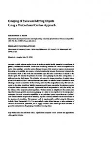
1. Introduction Current industrial manipulators suffer from ineffectiveness due to their inability to perform satisfactorily in a variety of situations. Current systems are often very brittle and fail due to changes in the environment, the manipulator, or the sensors. Typically, objects to be manipulated are required to appear in distinguished positions and at pre-defined orientations (often through the aid of fixtures), or are required to maintain stringent speed, location, and orientation restrictions. If these restrictions are not adhered to, then the system fails with no hope of recovery via sensing. Flexible manipulation of objects requires the use of sensors in order to determine salient properties of the object of interest and the robot’s workspace. Vision sensors (e.g., CCD cameras) have revolutionized the area of sensor-based robotics by introducing flexibility to conventional robotic systems [42]. The recent introduction of inexpensive and fast real-time image processing systems allows for the efficient integration of the visual sensory information in the feedback loop of a robotic system. Even though the robotic visual control area has drastically expanded in the recent years, its main focus has remained the visual tracking of objects by using the information gathered by static- or robot-mounted cameras [2][11][12][15][31][39][40][45]. This work, while important in its results and implications, has concentrated upon the active observation of the environment, leaving interaction as an issue for future research. In particular, only a small number of researchers [1][24][26][38] have proposed vision-based robotic systems that interact with the environment. We propose a flexible system based upon a camera repositioning controller operating under the Controlled Active Vision framework [31][34]. The controller permits the manipulator to robustly grasp objects in the workspace (see Figure 1). The system operates in an uncalibrated space with an uncalibrated camera. Moreover, the proposed scheme allows automatic planning and execution of all the necessary actions in order to grasp an object. The object of interest is not required Image
CCD Camera and Gripper
A
B C
Target D Image A´
B´
D´
C´
CCD Camera and Gripper Target Fig. 1.Experimental setup.
to appear in a specific location, orientation, or depth, nor is it required to remain motionless during the grasp. In this paper, we first present the previous work related to both the camera repositioning problem and the vision-based grasping problem. Next, we briefly discuss the visual measurements we have applied to this problem, elaborate on the use of “coarse” and “fine” features for guiding grasping, and discuss feature selection and reselection. We then describe the application of the Controlled Active Vision framework to the problem of servoing and repositioning around a target including a analysis regarding the stability of the controller. Next, an adaptation of this control paradigm to vision-based grasping of objects is given. We verify the operation of the system by presenting experimental results using the MRVT [7] system. The validity of the control paradigm is first validated in experiments where the camera is repositioned with respect to a static target. We then present results from experiments where the manipulator successfully grasps static objects using a vision-based, closed loop control strategy throughout the grasping task. We then extend this work to moving objects and present preliminary results of using the vision-based control approach to effect moving object grasping. Finally, we discuss the strengths and weaknesses of our approach, suggest required future work, and summarize our results. 2. Previous Work In the next sections, we present the previous work in the areas related to this paper. First, we discuss related research efforts on the camera repositioning problem. We then review the prior work regarding grasping using vision sensors, including relevant background in visually-guided robotics. 2.1. CAMERA REPOSITIONING The problem of robotic visual servoing around a target has been addressed by various researchers. Weiss et al. [44] have used a model reference adaptive control scheme in order to solve the problem. Their scheme has been verified by several simulations. Chaumette et al. [9][10] have proposed a method that combines a pre-computed Jacobian (from the target frame to the camera frame) with a simple adaptive control law. Four features are tracked by using simple line scanning techniques. The objective of their research is to make the robot-camera system reach a certain pose with respect to the static target. Hashimoto et al. [21] have presented a neural network based approach to the problem. The neural network learns the inverse perspective transformation after several trials using four feature points. The approach has been tested by running several simulations.
2.2. VISION-BASED GRASPING Several research efforts have focused on the problem of using vision information in the execution of several robot control tasks. Bennett et al. [4] described a system designed to locate a fuel inlet and attach a refueling boom for aircraft refueling. Luo et al. [28] have described a robot conveyor tracking system that incorporates a combination of visual and acoustic sensing. Nelson [30] has proposed a robotic visual tracking scheme that takes into consideration the robot joint limits and the singularities. Dickmanns [14] used vision to guide a vehicle that was driving down a highway. All of these systems applied visual information to the problem of robustly moving a robotic device within a reasonably defined workspace. In contrast, prior work in the use of visual information for grasping has resulted in only a limited number of systems. Many of these systems use a static camera and a calibrated coordinate transformation from the camera frame to the manipulator frame. Additionally, these systems typically use open-loop control, making these systems sensitive to errors in sensing, manipulator control, and calibration of the coordinate transformation. In particular, several efforts use vision only to gather information before performing a blind grasp, resulting in systems that cannot adapt to object motion. Houshangi [24] developed a system to grasp moving targets using a static camera and precalibrated camera-manipulator transform. Koivo [26] proposed a control theory approach for grasping using visual information. Allen et al. [2] presented a system that tracked a target moving in an oval path using calibrated, static stereo cameras and grasped the target when tracking became stable. Schrott [38] proposed a set of actions that an eye-in-hand system should do in order to grasp a static known object. Buttazzo et al. [8] used a calibrated static camera to determine when and where an object would cross a line defined by the intersection of the operating plane of the manipulator and the ground plane of the workspace. This information was used with open-loop control to place a basket mounted on the end-effector over the object when the object crossed the predefined line. Stansfield [41] used structured light to analyze object shape and size before performing a ballistic, unguided grasp. Several researchers have investigated catching and juggling (for example, [25][36][37]); however, these efforts consist mainly of open-loop control [25][36][37] and use vision sensors only to predict the parabolic trajectory of a dropping or tossed object [25][37] that is then used to blindly move the end-effector to a position along the parabola prior to the arrival of the object. 3. Measuring Coarse and Fine Feature Motion We must measure feature motion to visually guide the manipulator during the grasping process. Additionally, we introduce the concept of coarse and fine fea-
tures to compensate for the changes in features’ projections that result from the eye-in-hand robot reaching toward the target. As the reach is executed, coarse features will pass out of the view of the camera and will be replaced by fine feature. This also implies that features will be required to be automatically selected during the grasping process. Automatic reselection of features will also need to occur due to the visual distortion of features caused by the rotation of the camera and the change in depth of the features. This section addresses these issues in the context of vision-based grasping. 3.1. MEASUREMENTS We assume a pinhole camera model with a world frame { R S } fixed with respect to the camera and the Z-axis pointing along the optical axis. A point T P = ( X S, Y S, Z S ) in {RS} projects to a point p in the image plane with image coordinates x and y . For simplicity, we assume that δ x = δ y = f = 1 , where δ x and δ y are the scaling factors for pixel size and camera sampling and f is the camera focal length. By utilizing the derivation presented previously in [31][39][40], we arrive at the following equations describing the motion of p on the image plane due to P moving with translational motion t = ( t x, t y, t z ) T and rotational motion T r = ( r x, r y, r z ) : u = x = x v = y = y
tz t 2 – x + [ xyr x – ( 1 + x )r y + yr z ] ZW ZW
(3.1)
�
tz t 2 – y + [ ( 1 + y )r x – xyr y – xr z ] . ZW ZW
(3.2)
�
�
�
�
�
�
�
�
�
�
�
� �
�
�
�
�
�
�
�
�
�
�
�
�
� �
The continuous extraction of the positions of the features’ projections on the image plane is based on optical flow techniques. The computation of u and v (optical flow components) has been the focus of much research and many algorithms have been proposed [22][23][43]. We use a modified version of the matching based technique [3] also known as the Sum-of-Squared Differences (SSD) optical flow. For every point p A = ( x A, y A ) T in image A , we want to find the point p B = ( x A + u, y A + v ) T to which the point p A moves in image B . It is assumed that the intensity values in the neighborhood N of p A remain almost constant over time, that the point p B is within an area Ω of p A , and that velocities are normalized by the sampling period T to get the displacements. Thus, for the point p A the SSD estimator selects the displacement d = ( u, v )T that minimizes the SSD measure: e ( p A, d ) =
∑
m, n ∈ N
[ I A ( x A + m, y A + n ) – I B ( x A + m + u, y A + n + v ) ]
2
(3.3)
where u, v ∈ Ω , N is an area around the pixel we are interested in, and I A , IB are the intensity functions in images A and B , respectively. Variations of the previous technique are used in our experiments. In the first variation, image A is the first image ( k = 0 ) acquired by the camera while image B is the current image ( k > 0 ). Thus, for the point pA the SSD estimator selects the displacement d = ( u, v )T that minimizes the SSD measure: e ( p A, d ) =
∑
[ I A ( x A + m, y A + n ) – I B ( x A + m + u + ξu, y A + n + v + ξv ) ]
2
(3.4)
m, n ∈ N
where ξu and ξv are the sums of the all the previously measured displacements. They are defined as: ξu =
k–1
k–1
j=1
j=1
∑ u ( j ) and ξv =
∑ v( j) .
(3.5)
This variation of the SSD technique is sensitive to large rotations and changes in the lighting. Another variation of the SSD is the one that updates image A every µ images. This SSD measure is similar to the one previously mentioned (3.4) except that ξu and ξv are defined as: k–1
ξu =
∑
j = µl + 1
k–1
u ( j ), ξv =
∑
v ( j ), and l =
j = µl + 1
�
k . µ �
�
(3.6)
The most efficient variation of the SSD in terms of accuracy and computational complexity proved to be the last one [31]. The continuous computation of the displacement vectors helps us to continually update the coordinates of the image projections of the feature points. Additionally, this variation addresses our need to reselect features, as discussed in the Section 3.3.. The size of the neighborhood N must be carefully selected to ensure proper system performance. Too small an N fails to provide enough contrast while too large an N increases the associated computational overhead and enhances the background. In either case, an algorithm based upon the SSD technique may fail due to inaccurate displacements. To counter this, the system utilizes a technique called “dynamic pyramiding” as described in [39]. 3.2. COARSE AND FINE FEATURES We decompose the motion into coarse and fine segments by using two different classes of object features during operation. We use the idea of “coarse” and “fine” features during the operation of the system to guide the manipulator’s movements. Consider approaching a building that you wish to enter. At long distances, you use the building as a whole to guide your approach. This is analogous to the use of coarse features in our system to guide the early, coarse movements. Once you are near enough to the building to identify the entrance, the entrance itself becomes the guiding feature, while the entirety of the building is ignored. This is analogous
to the use of fine features in our system. When the object dominates the field of view of the camera, fine features are used to guide the manipulator motion. Coarse features are selected while the object is at relatively far distances from the end-effector. The system automatically aligns the gripper with the object and forces the optical axis of the camera to pass through the centroid of the object. It then drives the manipulator toward the object while maintaining proper gripper and optical axis alignment. When the object is in motion, these alignment constraints result in the tracking of the object by the manipulator. When the coarse features approach the boundaries of the image plane, fine features are selected. These are used to drive the end-effector the remaining distance to the object and to signal when to grasp the object using a pneumatic, two-fingered hand. Proper orientation is maintained throughout by visual information derived from either the coarse or the fine features, depending upon the type of features being used to guide the manipulator (see Figure 2). 3.3. FEATURE SELECTION/RESELECTION An algorithm based upon the SSD technique may fail due to repeated patterns in the intensity function of the image or due to large areas of uniform intensity in the image. Both cases can provide multiple matches within a feature point’s neighborhood, resulting in incorrect displacement measures. Furthermore, during certain movements of the manipulator (e.g., Z-axis translation and X-, Y-, or Z-axis rotations), the features being tracked will be distorted on the image plane, resulting in loss of tracking. In order to avoid these problems, our system automatically evaluates, selects, and reselects feature points (see Figure 2). Feature points are selected (and reselected) using the SSD measure combined with an auto-correlation technique. This produces an SSD surface that corresponds to an auto-correlation in the area Ω about a potential feature [3][31][40]. Several possible confidence measures can be applied to the surface to measure the suitability of a potential feature point. The selection of a confidence measure is critical since many such measures lack the robustness required by changes in illumination, intensity, etc. We use two-dimensional displacement parabolic fit that attempts to fit the parabola e ( ∆r ) = a∆r 2 + b∆r + c to a cross-section of the surface derived from the SSD measure [31]. The parabola is fit to the surface in several predefined directions. A Camera Alignment
Coarse Reach
Coarse Feature Selection
Fine Reach Fine Feature Selection
Feature reselection Fig. 2. Architecture for grasping.
Feature reselection
Close Gripper and Withdraw
feature point is selected if the minimum directional fit is sufficiently high, as measured by equation (3.4). After the coarse points are selected and the manipulator begins the centering and alignment phase, feature reselection is performed every µ th iteration in a small area Γ about each feature point using the method described above. This prevents loss of feature tracking due to distortions caused by the rotation about the Zaxis required to align the gripper with the graspable dimension of the object and the possible motion of the object. The reselection rate µ is based upon the maximum rate of the rotation about Z, the estimated motion of the object, and the expected velocity of the feature points on the image plane. reselection also takes place during the Z-axis translation that occurs while driving the manipulator toward the object. Once the coarse features are driven to points near the image plane edges, fine features are selected on the object’s surface. Only a small area in the center of the image plane is searched for fine features so that the projection of the points will remain within the bounds of the image plane during the final approach. Again, the features are reselected in a small area Γ about the points during the final approach in order to counter the effect of distortion due to the Z-axis translation and object motion. Since the velocities and distortions of the fine features are expected to be much higher due to the object’s short distance from the image plane (due to the small relative depth of the features), the reselection rate µ is set to force reselection more often during the fine feature approach. 4. Modeling of grasping as a visual servoing problem We address the problem of grasping (eye-in-hand configuration) as a visual servoing problem in this section. The grasping problem can be defined as “find the motion of the manipulator that will grasp a static or slowly moving object.” Since we are dealing with an eye-in-hand robotic system, we have to address the repositioning of the manipulator in order to effect grasping. The specific problem can be stated as “find the motion of the manipulator that will cause the image projections of certain feature points of the rigid target to move to desired image positions.” Contrary to previous research efforts [9][10], only partial knowledge of the inverse perspective transformation is assumed. In other words, vision-based grasping of an object by an eye-in-hand robotic system requires that the robot continuously repositions itself with respect to the object to be grasped. We accomplish this by automatically defining desired positions for the object features such that the robot aligns the end-effector with the object, reaches toward the object (while maintaining gripper/object alignment), and grasps the object.
4.1. MODELING APPROACH According to the derivation given in [35], we produce the following equations written in the state-space form (this model holds for static or slowly moving objects): (4.1) x F ( k + 1 ) = A F ( k )x F ( k )+ J F ( k – + 1 )u con ( k – + 1 )+ H F ( k )v F ( k ) �
�
where A F ( k ) = H F ( k ) = I 2 , x F ( k ) ∈ ℜ 2 , u con ( k ) ∈ ℜ 6 , v F ( k ) ∈ ℜ 2 , and sampling period. The matrix J F ( k ) ∈ ℜ2 × 6 is ( T is the sampling period): �
JF ( k ) = T
–1 Z s(k ) �
�
�
�
�
�
�
�
�
�
�
�
0
x(k ) 2 x ( k )y ( k ) – ( 1 + x ( k ) ) y ( k ) Z s(k ) –1 y ( k ) 2 ( 1 + y ( k ) ) – x ( k )y ( k ) – x ( k ) Z s(k ) Z s(k ) �
0
�
�
�
�
�
�
�
�
�
�
�
�
�
�
�
�
�
�
�
�
�
�
�
�
�
�
�
�
�
�
�
�
�
�
�
�
�
�
�
is the
.
x F ( k ) = ( x ( k ), y ( k ) )T is the state vector, T u con ( k ) = ( t x ( k ), t y ( k ), t z ( k ), r x ( k ), r y ( k ), r z ( k ) ) is the control input vector, and v F ( k ) = ( v 1 ( k ), v 2 ( k ) ) T is the white noise vector. The measurement vector T y F ( k ) = ( y 1 ( k ), y 2 ( k ) ) for this feature is given by:
The
vector
yF ( k ) = CF xF ( k ) + wF ( k )
(4.2)
where w F ( k ) = ( w 1 ( k ), w 2 ( k ) ) is a white noise vector, ( w F ( k ) ∼ N ( 0, W ) ) , and C F = I 2 . The measurement vector is computed using the SSD algorithm described in Section 3.. One feature point is not enough for the calculation of the control input vector u con ( k ) due to the fact that the number of outputs is less than the number of inputs. Thus, we are obliged to consider more points in our model. In order to make the number of inputs equal to the number of outputs, we must consider at least three feature points which are not collinear. The reason for the noncollinearity will be investigated in Section 4.2.. Having more than three feature points will result in a larger number of outputs than inputs. In repositioning, the robot-camera system is not required to take a certain pose with respect to the static rigid target. The only objective is to move a certain number of features to some desired positions on the image plane. Additional objectives such as a predefined pose require at least four feature points [9]. When we introduce grasping based upon this concept (see Section 4.3.), our camera pose will be predefined and the controller will use four feature points. In our formulation the depth parameter of each one of the feature points is estimated on-line by an adaptive estimator, and therefore, the relative position of the object with respect to the robot-camera system can be computed. The state-space model for three feature points is very similar to that found in [35] for m points and can be written as: x ( k + 1 ) = A ( k )x ( k ) + J ( k – + 1 )u con ( k – + 1 ) + H ( k )v ( k ) (4.3) T
�
�
where A ( k ) = H ( k ) = I 6 , and v ( k ) ∈ ℜ 6 . The matrix J ( k ) ∈ ℜ 6 × 6 is:
(1)
JF ( k ) J ( k ) = J (F2 ) ( k ) . (3)
JF ( k )
The superscript ( i ) denotes each one of the feature points ( ( i ) ∈ { ( 1 ) , ( 2 ), (1) (1) (2) (2) (3) (3) ( 3 ) } ) . The vector x ( k ) = ( x ( k ), y ( k ), x ( k ), y ( k ), x ( k ), y ( k ) )T (1) (1) is the new state vector, and v ( k ) = ( v 1 ( k ), v 2 ( k ), (2) (2) (3) (3) T is the new white noise vector. The new v 1 ( k ), v 2 ( k ), v 1 ( k ), v 2 ( k ) ) (1) (1) (2) (2) (3) measurement vector y ( k ) = ( y 1 ( k ), y 2 ( k ), y 1 ( k ), y 2 ( k ), y 1 ( k ), (3) T y 2 ( k ) ) for three features is given by: (4.4) y ( k ) = Cx ( k ) + w ( k ) T (1) (1) (2) (2) (3) (3) where is the w ( k ) = ( w 1 ( k ), w 2 ( k ), w 1 ( k ), w 2 ( k ), w 1 ( k ), w 2 ( k ) ) new white noise vector ( w ( k ) ∼ N ( 0, W ) ) and C = I 6 . More feature points can be integrated in our model by augmenting the block matrix J ( k ) and the measurement, state, and white noise vectors. We can combine equations (4.3)-(4.4) into a MIMO (Multi-Input Multi-Output) ARX (AutoRegressive with auXiliary input) model. This model consists of six MISO (Multi-Input Single-Output) ARX models, and is described by the following equation: A ( k ) ( 1 – q )y ( k ) = J ( k – –1
)u con ( k –
) + n(k )
(4.5) where n ( k ) is the white noise vector and q is the backward shift operator. The new white noise vector n ( k ) corresponds to the measurement noise, modeling errors, and noise introduced by inaccurate robot control. In the next section, we present the control and estimation techniques for the repositioning problem. �
�
–1
4.2. CONTROL, ESTIMATION, AND STABILITY FOR REPOSITIONING The control objective is to move the manipulator in such a way that the projections of the selected features on the image plane move to some desired positions [32]. This section presents the control strategies that realize this motion, the estimation scheme used to estimate the unknown parameters of the model, and the stability analysis of the proposed visual servoing algorithms. Since the depth information is not directly available, adaptive control techniques are used for visually servoing around a object. In particular, adaptive control techniques are used for the recovery of the components of the translational and rotational velocity vectors t ( k ) and r ( k ) , respectively. The rest of the section will be devoted to the detailed description of the control and estimation schemes. 4.2.1.
Control scheme for repositioning
The objective is to move the features’ projections on the image plane to some desired positions. The repositioning of the projections is realized by an appropri-
ate motion of the camera. The design of this controller is similar to the one proposed in [35]. By transforming our objective to a cost function, we can create a mathematical formula that continuously computes the desired motion of the camera. This motion is transformed through a robot control scheme to robot motion. In particular, a simple control law can be derived by the minimization of a cost function that includes the control signal [27]: (k + �
) = [y(k + �
) – y des ( k + �
+u
T con
�
) ] GM [ y ( k + T
�
) – y des ( k + �
)]
( k )G I u con ( k ).
(4.6)
The vector y des ( k ) represents the desired positions of the projections of the three features on the image plane. In our repositioning experiments, the vector y des ( k ) is known a priori and is constant over time. However, during certain stages of the grasping the vector y des ( k ) is known but time-varying. By weighting the control signal, we place some emphasis on the minimization of the control signal in addition to the minimization of the servoing error. The response of the system is slower than having G I = 0 but the control input signal is bounded and feasible. This is in agreement with the structural and operational characteristics of the robotic system and the vision algorithm. A robotic system cannot track signals that command large changes in the features’ image projections during the sampling interval T . The control law which is derived from the minimization of the cost function (4.6) is: –1 T
u con ( k ) = – [ J ( k )G M J ( k ) + G I ] J ( k )G M { [ y ( k ) – y des ( k + T
�
–1
+ ∑ J ( k – m )u con ( k – m ) }.
�
)]
(4.7)
m=1
The design parameters in this control law are the elements of the matrices G M and G I . The matrix G M should be positive definite ( G M > 0 ) while G I should be positive semidefinite ( G I ≥ 0 ). If the matrix J ( k ) is full rank then the matrix T J ( k )G M J ( k ) + G I is invertible. The matrix J ( k ) is singular when the three feature points are collinear (see [16] for a detailed discussion of this case). This is similar to the work presented in [35] that extends the number of points to m . For grasping, we will extend the number of points to four (see Section 4.3.). In addition, J ( k ) becomes singular if Z (s1 ) ( k ) = Z (s2 ) ( k ) = Z (s3 ) ( k ) and at least one of the feature points has a projection on the image plane with coordinates x ( i ) ( k ) = y ( i ) ( k ) = 0 ( ( i ) ∈ { ( 1 ), ( 2 ), ( 3 ) } ). Moreover, J ( k ) becomes singular if the three feature points and the origin of the camera frame O belong to the same cylinder and the following condition is satisfied [13]: (1)
�
(2)
(3)
OO OO OO = = = γ1 . (1) (2) (3) tan ( β ) tan ( β ) tan ( β ) �
�
�
�
�
�
�
�
�
�
�
�
�
�
�
�
�
�
�
�
�
�
�
�
�
�
�
�
�
�
�
�
�
�
�
�
�
�
�
�
�
�
�
�
�
�
�
�
�
�
�
�
�
�
�
�
�
�
�
�
�
�
(4.8)
Each angle β ( i ) ( – π ⁄ 2 < β ( i ) < π ⁄ 2 ) corresponds to the ( i ) feature and is defined as shown in Figure 3. Moreover, OO ( i ) denotes the signed magnitude of the vector (i) OO . If β ( i ) = 0 for every feature point, then γ 1 = ± ∞ . This fact implies that the three feature points and the origin of the camera frame O belong to the same line.
C (i) P (i)
β (i)
β (i) O (i) Fig. 3. Definition of the angle β
(i)
.
Ys C
(2)
C
(1)
Ys (3) C C(2) P (3)
O(2) P (2) P (1)
Zs Xs P (3) C(3)
O(1)
C(1)
O
Zs Xs
O(3)
P (1) P (2) (2) O O O(1)
O(3)
(b)
(a)
Fig. 4. The axis of the cylinder is parallel to the (a) Y axis and (b) X axis of the camera frame.
If β ( i ) = π ⁄ 2 or O = O ( i ) for every feature point, then γ 1 = 0 . The fact that (i) β = π ⁄ 2 for every feature point implies that the three feature points belong to the same line (a case that was examined earlier). Two particular cases of the previous conditions are shown in Figure 4. In the first case (the axis of the cylinder is parallel to the Y axis of the camera frame), the fact that the three feature points and the origin of the camera frame O belong to the same cylinder can be described as: (1)
(1)
2
(2)
(2)
2
[ ( x ( k ) ) + 1 ]Z s ( k ) = [ ( x ( k ) ) + 1 ]Z s ( k ) = (3)
(3)
2
[ ( x ( k ) ) + 1 ]Z s ( k ) = γ 2 .
(4.9)
Moreover, equation (4.8) can be simplified as: (1)
(1)
(2)
(1)
(2)
(2)
x ( k )y ( k )Z s ( k ) = x ( k )y ( k )Z s ( k )= (3)
(3)
(3)
x ( k )y ( k )Z s ( k ) = γ 1 .
(4.10)
In the second case (the axis of the cylinder is parallel to the X axis of the camera frame), the fact that the three feature points and the origin of the camera frame O belong to the same cylinder can be described as: (1)
(2)
(1)
2
2
(2)
[ ( y ( k ) ) + 1 ]Z s ( k ) = [ ( y ( k ) ) + 1 ]Z s ( k ) = (3)
2
(3)
[ ( y ( k ) ) + 1 ]Z s ( k ) = γ 3 .
(4.11)
Moreover, equation (4.8) can again be simplified to equation (4.10). A proof that the above conditions make J ( k ) singular can be found in [13] and in [31]. It should be mentioned that a similar analysis has been performed in [16]. By selecting G I and G M , one can place more or less emphasis on the control input and the servoing error. By following the results in [35], we can select the elements of these matrices. If we want to include the noise of our model and the inaccuracy of the J ( k ) matrix in our control law, the control objective (4.6) will become: �
(k +
) = E {[y(k + �
) – y des ( k + �
+u
�
) ] GM [ y ( k + T
) – y des ( k + �
)] �
(4.12)
( k )G I u con ( k ) F k }
T con
where the symbol E { X } denotes the expected value of the random variable X and F k is the sigma algebra generated by the past measurements and the past control inputs up to time k . The new control law is: –1 T
T
u con ( k ) = – [ J ( k )G M J ( k ) + G I ] J ( k )G M { [ y ( k ) – y des ( k + �
�
�
�
�
)]
(4.13)
–1
+ ∑ J ( k – m )u con ( k – m ) } �
m=1
where J ( k ) is the estimated value of the matrix J ( k ) . The matrix J ( k ) is depen(i) dent on the estimated values of the features’ depth Zs (k) ( ( i ) ∈ { ( 1 ), ( 2 ), ( 3 ) } ) and the coordinates of the features’ image projections. In particular, the matrix J ( k ) is defined as follows: �
�
�
�
(1)
JF ( k ) �
J ( k ) = J (F2 ) ( k ) �
�
(3)
JF ( k ) �
(i )
where J F ( k ) is given by: �
(i )
JF ( k ) = �
(i)
–1 �
�
�
�
�
�
�
�
�
�
�
�
�
�
T Z (k) �
0
x (k)
0
�
(i) s
�
�
�
�
�
�
�
�
�
�
�
�
�
�
�
�
�
�
�
�
�
(i)
–1 �
�
Z (k) �
�
�
(i) s
�
�
�
�
�
�
y (k)
(i)
�
�
�
�
�
�
�
(i)
�
�
�
�
�
�
�
Zs (k) Zs (k) �
(i)
(i)
(i)
2
(i)
x ( k )y ( k ) – [ 1 + ( x ( k ) ) ] y ( k )
. (i)
2
(i)
(i)
(i)
[ 1 + ( y ( k ) ) ] – x ( k )y ( k ) – x ( k )
�
(i )
(i)
This matrix uses the estimated depth ( 1 ⁄ Z s ( k ) ) in the calculation of J F ( k ) . In the next section, we present estimation techniques for estimating the depth factor. �
�
4.2.2.
(i )
Computation of J F ( k ) through the estimation of 1 ⁄ Z (si ) ( k ) �
The estimation of the feature’s depth Z (si ) ( k ) with respect to the camera frame can be done in multiple ways. In this section, we present one estimation algorithm. Many more similar algorithms can be found in [35]. Let us define the inverse of the depth Z (si ) ( k ) as ζ (si ) ( k ) . Then, the equations (4.1)-(4.2) of each feature point can be rewritten as ( n(Fi ) ( k ) ∼ N ( 0, N ( i ) ( k ) ) ): (i )
(i )
(i )
(i)
y F ( k ) = A F ( k – 1 )y F ( k – 1 ) + ζ s ( k – (i) F2
+J ( k –
)r ( k – �
�
)J (F1i ) ( k –
)t ( k – �
(i ) F
) + n (k) �
�
)
(4.14)
where J (F1i ) ( k ) and J (F2i ) ( k ) are given by: (i)
(i) J F1 ( k ) = T – 1 0 x ( k ) , (i) 0 –1 y ( k )
J (F2i ) ( k ) = T
(i)
(i)
(i)
(i)
2
x ( k )y ( k ) – [ 1 + ( x ( k ) ) ] y ( k ) (i)
(i)
2
(i)
.
(i)
[ 1 + ( y ( k ) ) ] – x ( k )y ( k ) – x ( k )
By following methods in [35], the new form is: (i ) (i) (i) (i ) (4.15) ∆y F ( k ) = ζ s ( k – )u t ( k – ) + n F ( k ) . (i ) (i) The vectors ∆y F ( k ) and u t ( k – ) are known every instant of time, while the (i) scalar ζ s ( k ) is continuously estimated. It is assumed that an initial estimate 2 (i) (i) (i) (i) (i) is a positive ζ s ( 0 ) of ζ s ( 0 ) is given and p ( 0 ) = E { [ ζs ( 0 ) – ζs ( 0 ) ] } scalar p 0 . The term p ( i ) ( 0 ) can be( i )interpreted as a measure of the confidence that we have in the initial estimate ζ s ( 0 ) . Accurate knowledge of the scalar ζ (si ) ( k ) corresponds to a small covariance scalar p 0 . In our examples, N ( i ) ( k ) is a constant predefined matrix. In addition, for simplicity in notation, h ( k ) is used instead of (i) ut ( k ) . The estimation equations are (the superscript ′ – ′ denotes the predicted value of a variable while the superscript ′ + ′ denotes its updated value) [29]: �
�
�
�
�
�
- (i) s
+ (i)
ζ ( k ) = ζs ( k – 1 ) �
(4.16)
�
- (i)
+ (i)
(i)
p (k) = p (k – 1) + s (k – 1) + (i)
- (i)
–1
p (k) = [{ p (k)} + h (k – + (i)
k ( k ) = p ( k )h ( k – T
+ (i) s
- (i) s
T
�
T
(i)
(4.17) �
){N (k )} h(k –
){N (k )} (i )
(i)
–1
–1
)]
–1
(4.18) (4.19)
- (i) s
ζ ( k ) = ζ ( k ) + k ( k ) [ ∆y F ( k ) – ζ ( k )h ( k – T
�
)]
(4.20) where s ( k ) is a covariance scalar which corresponds to the white noise that characterizes the transition between the states. The depth related parameter (i) ζ s ( k ) is a time-varying variable since the camera translates along its optical axis and rotates about the X and Y axis. The estimation scheme of equations (4.16)-(4.20) can compensate for the time-varying nature of ζ s ( i ) ( k ) because it is �
�
(i)
�
�
designed under the assumption that the estimated variable undergoes a random change. Further analysis is given in [18] and [35]. 4.2.3.
Stability analysis
In this section we present an outline of a stability analysis for the proposed algorithms. Our objective is to investigate the conditions under which the servoing error ( e ( k ) = y ( k ) – y des ( k ) ) asymptotically goes to zero while the system input vector u con ( k ) and the system output vector y ( k ) remain bounded. In 1980, Goodwin et al. [19][20] dealt with the stability analysis of adaptive algorithms for discrete-time deterministic time-invariant MIMO systems. Using Goodwin’s work as a base, we outline the stability analysis for our discrete-time stochastic nonlinear slowly time-varying MIMO system. In this analysis, the 2-norm of a matrix L , often called the spectral norm, is used. This norm is defined as follows [46]: 1
Lx 2 2 T = ( maximum eigenvalue of L L ) ( x ≠ 0 ) . x 2 �
L
2
= max �
�
�
�
�
�
�
�
�
�
�
�
�
(4.21)
� �
The minimum and maximum eigenvalues of the matrix L are defined as λ max ( L ) and λ min ( L ) , respectively. For a deterministic version of our model (white noise is ignored) and for a system delay = 1 , the error equation is ( y des ( k ) is known a priori and is constant over time): (4.22) e ( k + 1 ) = [ I 6 – J ( k )M ( k ) ]e ( k ) �
where M ( k ) is defined as: –1 T
T
M ( k ) ≡ [ J ( k )G M J ( k ) + G I ] J ( k )G M �
�
.
�
(4.23)
The servoing error goes asymptotically to zero if the following condition holds: (4.24) I 6 – J ( k )M ( k ) 2 < 1 . The previous condition can be rewritten as: λ max ( I 6 – J ( k )M ( k ) – M ( k )J ( k ) + M ( k )J ( k )J ( k )M ( k ) ) < 1 T
T
T
T
.
(4.25)
After some simple matrix computations, condition (4.25) is transformed to: λ min ( J ( k )M ( k ) + M ( k )J ( k ) – M ( k )J ( k )J ( k )M ( k ) ) > 0 T
T
T
T
.
(4.26)
Therefore, the matrix J ( k )M ( k ) + M ( k )J ( k ) – M ( k )J ( k )J ( k )M ( k ) should be strictly positive definite. In the case that G I = 0 , the following condition should hold: T
–1
T
T
T
T
–1
T
J ( k )J ( k ) + { J ( k ) }–1 J ( k ) – { J ( k ) }–1 J ( k )J ( k )J ( k ) > 0 �
�
T
�
T
�
.
(4.27)
In continuous time, the condition becomes simpler. Chaumette et al. state [10] that –1 the matrix J ( t )J ( t ) should be positive definite. For > 1 , the error equation is more complex than the case of unit delay because previous control input vectors are included. The new error equation is given by: �
�
e ( k + 1 ) = [ I6 – J ( k + 1 – +J ( k + 1 – �
�
�
)M ( k + 1 –
)M ( k + 1 –
�
) ]e ( k )
) �
(4.28)
–1
∑ [J(k + 1 – �
– m) – J(k + 1 – �
�
– m ) ]u con ( k + 1 – �
– m ).
m=1 –1
The M ( k ) is again given by (4.23). For G I = 0 , M ( k ) is equal to J ( k ) . This implies that if J ( k ) asymptotically goes to J ( k ) , then the servoing error asymptotically goes to zero. This can be concluded from the error equation (4.28). In order for J ( k ) to converge to J ( k ) , the input signal u con ( k ) should be Persistently Exciting (PE). Goodwin [18] proposed several methods for creating persistently exciting input signals. In other words, the robot servoing motion can be slightly modified in order for the servoing error e ( k ) = y ( k ) – y des ( k ) to asymptotically go to zero. This issue is currently under investigation. It should be also stated that the problem of parameter convergence was extensively studied in [5][6]. More complete stability proofs can be created by using discrete Lyapunov functions and the properties of the estimation scheme. In this way, we can guarantee stability of the adaptive control algorithms under weaker conditions. The proper selection of initial and target feature points as well as the selection of G I , along with the careful design of the estimation scheme can guarantee continuous T nonsingularity of the matrix J ( k )G M J ( k ) + G I as described in Section 5.. �
�
�
�
4.2.4.
�
Implementation issues
In the experiments, we are forced to bound the input signals in order to avoid saturation of the actuators. Thus, both the translational velocity vector T t ( k ) = ( t x ( k ), t y ( k ) , t z ( k ) ) and the rotational velocity vector T r ( k ) = ( r x ( k ), r y ( k ), r z ( k ) ) are normalized to t′ ( k ) and r′ ( k ) , respectively, after their computation by following the methods in [35]. Thus, our controller design is very similar to the one presented therein. Accordingly, we must use the modified components of the translational and rotational velocity vectors for the computation of the past input signals u (t i ) ( k ) and u (ri ) ( k ) . Thus, instead of using the u (t i ) ( k ) and u (ri ) ( k ) signals in the estimation process, we use the signals u (t i ) ( k ) and u (ri ) ( k ) which are given by: (i)
(i)
(i)
(i)
u t ( k ) = J F1 ( k )t′ ( k ) and u r ( k ) = J F2 ( k )r′ ( k )
.
After the computation of the translational velocity vector t′ ( k ) and the rotational velocity vector r′ ( k ) with respect to the camera frame { R s } , we transform them to the end-effector frame { R e } with the use of the transformation e T s . The transformed signals are fed to the robot controller. The selection of the appropriate robot control method is essential to the success of our algorithms because small oscillations can blur the acquired images. Blurring reduces the accuracy of the visual measurements and as a result the system cannot accurately servo around the object.
4.3. MANIPULATOR CONTROL FOR GRASPING Manipulator motions are effected by a control law similar to that in the previous sections: –1 T
T
u con ( k ) = – [ J ( k )G M J ( k ) + G I ] J ( k )G M { [ y ( k ) – y des ( k + �
�
�
�
�
)] +
–1
∑ J ( k – m )u �
con
( k – m ) }.
m=1
We use this control law during both the object centering and gripper alignment phase, and the object approach and grasping phase. We also extend the use of the controller to the grasping of moving objects since we consider slowly moving targets. If the speeds of the object increase, the control law can be easily modified to include the motion of the object as a disturbance term. The values of y des ( k ) are held constant during the centering and alignment phase and are timevarying during the approach phase. During approach, several intermediate values of the desired feature point locations are automatically calculated. These intermediate values are used to smoothly guide the gripper to the object and to maintain gripper alignment throughout the approach and grasping phase (see Figure 5). Even when the object is in motion, the alignment and centering requirements of the controller cause the manipulator to track the motion, resulting in a system that can grasp objects inspite of the motion of those objects. 5. Experimental Results 5.1. THE MRVT HARDWARE We have implemented our system using the Minnesota Robotic Visual Tracker (MRVT) (see Figure 6) [7]. The MRVT is a multi-architectural system which con-
Tracking Windows
Target
Successive ydes(k)’s
Fig. 5. Desired feature positions.
Sun 4/330
RCS
B I T 3
VPS
VME I B V B I 3 I T 2 T 3 3 3 0
Datacube M a MBM a 1 I x x 4 T 2 8 7 3 0 6 0
CCD Camera Unimation Controller
Arm/Controller Cable Gripper Control Line
Fig. 6. MRVT system architecture.
sists of two main parts: the Robot/Control Subsystem (RCS) and the Vision Processing Subsystem (VPS). The RCS consists of a PUMA 560 manipulator, its associated Unimate Computer/Controller, and a VME-based Single Board Computer (SBC). The manipulator’s trajectory is controlled via the Unimate controller’s Alter line and requires path control updates once every 28 msec. Those updates are provided by an Ironics 68030 VME SBC running Carnegie Mellon University’s CHIMERA real-time environment. A Sun SparcStation 330 serves as the CHIMERA host and shares its VME bus with the Ironics SBC via BIT-3 VME-to-VME bus extenders. The VPS receives input from a Panasonic GP-KS102 miniature camera that is mounted parallel to the end-effector of the PUMA and provides a video signal to a Datacube system for processing. The Datacube is the main component of the VPS and consists of a Motorola MVME-147 SBC running OS-9, a Datacube MaxVideo20 video processor, a Datacube Max860 vector processor, and a BIT-3 VME-to-VME bus extender. The bus extender allows the VPS and the RCS to communicate via shared memory, eliminating the need for expensive serial communication. The VPS performs the optical flow, calculates the desired control input, and supplies the input vector via shared memory to the Ironics processor for inclusion as an input into the control software. The video processing and calculations required to produce the desired control input are performed under a pipeline programming model using Datacube’s Imageflow libraries. Additionally, a serial port on the MVME-147 is dedicated to gripper control. When the VPS identifies that the conditions required for grasping have been met, it signals the Unimate Controller to close the gripper via an inexpensive, custom hardware interface. 5.2. CAMERA REPOSITIONING The theory was verified by performing a number of experiments. The focal length of the camera is 7.5 mm and the objects are static (the initial depth of the objects’
center of mass with respect to the camera frame Z s is varying from 400 mm to 1000 mm). The camera’s pixel dimensions are: δ x = 0.01278 mm/pixel and δ y = 0.00986 mm/pixel. The maximum permissible translational velocity of the end-effector is 10 cm/sec and each one of the components (roll, pitch, yaw) of the end-effector’s rotational velocity must not exceed 0.05 rad/sec. Our objective is to move the manipulator so that the image projections of features of the object move to desired positions in the image. The objects used in the servoing examples include books, pencils, and in general items with distinct features Figure 7. The user, with the use of the mouse, proposes to the system some of the object’s features. Then, the system evaluates on-line the quality of the features based on the confidence measures described in [33]. The same operation can be done automatically by a computer process that runs once for approximately 0.5 to 3 seconds, depending on the size of the interest operators which are used. The three (minimum number of required features for full motion of the manipulator) best features are selected and used for the robotic visual servoing task. The size of the windows is 10x10. The experimental results are presented in Figures 9 through 14. The gains for the controllers are and GM = I6 G I = diag { 0.025, 0.025, 0.25, 5 5 5 2 × 10 , 2 × 10 , 2 × 10 } . The delay factor d is 2. The computation of the T –1 matrix is done on a MVME-147 68030 board. We use two [ J ( k )G M J ( k ) + G I ] different techniques for its computation. The first technique performs a Singular Value Decomposition (SVD) of the 6x6 matrix based on a routine given by Forsythe [17] and has a computational time of 30 ms. This routine uses techniques such as the Householder reduction to bidiagonal form and diagonalization by the QR method. The computation of the inverse is based on the results of the SVD routine. The second technique is based on the partition of the matrix T K ( k ) = J ( k )G M J ( k ) + G I into four submatrices [16][18]: �
�
�
K(k ) =
�
K 11 ( k ) K 12 ( k ) K 21 ( k ) K 22 ( k )
.
Goodwin [18] shows that the inverse of K ( k ) is given by: K (k) =
N2 ( k )
– N 2 ( k )K 12 ( k )K 22 ( k )
–1
–1
–1
– N 1 ( k )K 21 ( k )K 11 ( k ) –1
–1
–1
N1 ( k ) –1
(5.1)
where
N 1 ( k ) = K 22 ( k ) – K 21 ( k )K 11 ( k )K 12 ( k ) –1
and
N 2 ( k ) = K 11 ( k ) – K 12 ( k )K 22 ( k )K 21 ( k ) . –1
We can reduce the complexity of matrix inversions by using simple matrix algebra and the matrix inversion lemma [18]. Therefore, we can derive a new form for K –1 ( k ) that requires only the inversion of two 3x3 matrices [16]:
K (k) = –1
K 11 ( k ) { I 3 + K 12 ( k )N 1 ( k )K 21 ( k )K 11 ( k ) } K 11 ( k )K 12 ( k )N 1 ( k ) –1
–1
–1
–1
–1
– N 1 ( k )K 21 ( k )K 11 ( k ) –1
N1 ( k )
–1
–1
.
By using the previous form, we are able to reduce the computational time of the 6x6 matrix inversion to 10 ms. Thus, the total computation time (image processing and control calculations) of t′ ( k ) and r′ ( k ) is approximately 50 ms. The inversion of the two 3x3 submatrices is done based on the assumption that the submatrices are invertible. Thus, the singularity of the submatrices should be checked every period T . The initial and the estimated values of the coefficients of the ARX models are given in the Table I and Table II. In the first example (Figures 9 through 11), we check the efficiency of the proposed estimation scheme (plotted as errors in X and Y on the image plane). In Figures 12 through 14, one can observe the results from the application of our method in another servoing example. TABLE I. Initial and estimated values of the parameters for the first example of servoing. (1)
(2)
(3)
(1)
(2)
(3)
ζs ( k )
ζs ( k )
ζs ( k )
p (k)
p (k)
p (k)
Initial
0.4175
0.4175
0.4175
0.1
0.1
0.1
Estimated
0.9435
0.9389
0.8594
0.0015
0.0014
0.0014
TABLE II. Initial and estimated values of the parameters for the second example of servoing. (1)
(2)
(3)
(1)
(2)
(3)
ζs ( k )
ζs ( k )
ζs ( k )
p (k)
p (k)
p (k)
Initial
0.4175
0.4175
0.4175
0.1
0.1
0.1
Estimated
0.7876
0.8298
0.7715
0.0010
0.0011
0.0011
(b)
(a)
Fig. 7. Initial (a) and final (b) images of the target in the first example.
(a)
(b)
Fig. 8. Initial (a) and final (b) images of the target in the second example.
Error (Pixels)
�
250 �
X component Y component
200 �
150 100 50 �
0 �
10
20
30
40
50
60
70
80
90
100
Time (Seconds) Fig. 9. Servoing errors for the first feature (A) in the first example. The depth related parameter -50
(i)
ζ s ( k ) of each feature point is estimated by taking into consideration both the measurements in the X and Y directions.
Error (Pixels)
�
250 �
X component Y component
200 �
150 100 50 �
0 �
10
20 �
30
40
50 �
60 �
70 �
80 �
90 �
100 �
Time (Seconds) -50 Fig. 10. Servoing errors for the second feature (B) in the first example. The depth related parameter
(i)
ζ s ( k ) of each feature point is estimated by taking into consideration both the measurements in the X and Y directions.
Error (Pixels)
�
250
X component Y component
200 �
150 100 �
50 0 �
10
20 �
30 �
40 �
50 �
60 �
70 �
80 �
90 �
100 �
Time (Seconds) -50 Fig. 11. Servoing errors for the third feature (C) in the first example. The depth related parameter �
(i)
ζ s ( k ) of each feature point is estimated by taking into consideration both the measurements in the X and Y directions.
Error (Pixels)
�
150
X component Y component
�
100 50 0 �
10
-50
20
30 !
40 "
50 #
60 $
70 %
80 &
90 '
100 �
Time (Seconds) (
�
-100 -150
Fig. 12. Servoing errors for the first feature (A) in the second example. The depth related parameter (i)
ζ s ( k ) of each feature point is estimated by taking into consideration both the measurements in the X and Y directions.
Error (Pixels)
�
150
X component Y component
�
100 �
50 0
10
20
30
40
50
60
70
80
90
100
Time (Seconds)
-50
(
�
-100 �
-150
Fig. 13. Servoing errors for the second feature (B) in the second example. The depth related (i)
parameter ζ s ( k ) of each feature point is estimated by taking into consideration both the measurements in the X and Y directions.
Error (Pixels)
�
100
X component Y component
50 �
0 �
10
20
30 !
-50
40 "
50 #
60 $
70 %
80 &
90 '
100 �
Time (Seconds) (
-100 -150 �
-200 �
Fig. 14. Servoing errors for the third feature (C) in the second example. The depth related parameter (i)
ζ s ( k ) of each feature point is estimated by taking into consideration both the measurements in the X and Y directions.
5.3. STATIC OBJECT GRASPING For grasping tasks, we assume that the object of interest is a rectangular prism with at least one linear dimension that fits into the span of the gripper fingers. We also assume that there are some surface markings that provide suitable fine features for the approach and grasping phase. We conducted several sets of experiments using the MRVT [7] by varying object’s beginning position, orientation, depth, and motion. The results from three of these sets of experiments are included. The first sets of experiments were conducted using a static object. Once we were satisfied with the system’s performance in these static tests, we allowed the object to exhibit translational motion throughout both the object centering and gripper alignment phase, and the object approach and grasping phase.
Fig. 15. Initial object position, camera view.
The first set of experiments was conducted by placing the object approximately 380 mm in depth, 18 mm from the optical axis of the camera, and at a rotation of 30° about the object’s Z-axis (see Figure 15). The system first aligns the gripper with the minimal linear dimension of the object and forces the optical axis to pass through the centroid of the object. Figures 16 and 17 show the manipulator’s X- and Y-axis translation with respect to the original camera coordinate frame, demonstrating the alignment of optical axis and the object centroid during the early potions of the plots, while Figure 18 clearly shows the manipulator’s rotation needed to align the gripper with the minimal linear dimension of the
Distance (mm)
20 15 10 5
1000
2000
3000
4000
5000
Distance (mm)
Time (cycles) Fig. 16. X-axis translation. 20 15 10 5
1000
2000
3000
4000
5000
Time (cycles) Fig. 17. Y-axis translation.
Rotation (deg)
Time (cycles) 1000
2000
3000
4000
5000
-5 -10 -15 -20 -25 -30
Fig. 18. Z-axis rotation.
object. In these plots, the time axis is given in cycles that correspond to the cycle time of the robot’s controller (28 msec) while the distance axis is given in mm of displacement or degrees of rotation relative to the original end-effector coordinate frame of the Puma. Figure 17 shows a significant overshoot in Y due to the unfinished rotation about the Z-axis. As the rotation proceeds, both X and Y translations show camera drift that is corrected when the rotation is near completion. During the remainder of these plots, object alignment (both with the gripper and the optical axis) are updated as the system is able to measure the position of the features more accurately. The plots reflect the minor adjustments made during the approach along the Z-axis. It is precisely this type of adjustment that visual sensing enables, leading to more accurate approaches and more robust grasping. These adjustments cannot be made by either a system without sensing or a system using sensing only to determine pose and then executing a blind grasp. It should be noted that the system must assume that the coarse feature points are the corners of the object in order to identify the minimal linear dimension and perform the alignment. The system then calculates several intermediate points ( y des ( k ) ’s) to guide the manipulator toward the object (see Figure 5). When the calculated positions for the desired points (the y des ( k ) ’s) near the image boundary, fine features are automatically selected and used to guide the continued approach of the manipulator. Figure 19 shows the approach of the manipulator along the Z-axis (approximated by the optical axis). Distance (mm)
Grasping occurs
300 200 100 1000
2000
3000
4000
5000
Time (cycles) Fig. 19. Z-axis translation.
In this preliminary version of the system, the size of the colored square that supplies the fine features is known, thereby allowing the system to predict the final positions of the fine features in order to allow grasping. However, the system selects these fine features automatically and their initial positions are unknown and are dependent upon the movements of the manipulator during the coarse guidance. Once the system has identified that the conditions required for grasping have been met and the gripper has been closed, the manipulator withdraws along the Zaxis, as shown near the end of the plot in Figure 19. Figure 20 shows the view from the end-effector when the system has determined that grasping should take place. An oblique view from outside the manipulator’s workspace (see Figure 21) clearly shows that the minimal dimension of the object falls within the span of the gripper fingers with only a small tolerance on each side for control error and noise. Had the system simply relied upon the gripper and optical axis alignment of the first stage, the accuracy needed to grasp a wide object such as this box would not have been available and the failure rate of the system would have been much higher. The second set of experiments we present was conducted using an initial configuration significantly different from the first set. A different object was placed
Fig. 20. Manipulator view at grasping.
Fig. 21. Oblique view at grasping.
Fig. 22. Initial object position, camera view.
approximately 81 mm off the optical axis and at a rotation of – 6° about the object’s Z-axis (see Figure 22). The manipulator was approximately 600 mm above the object.
Distance (mm)
Again, the gripper alignment and the alignment of the object centroid with the optical axis were performed during the initial stage of the process, as exhibited in Figures 23 through 26. The overshoot in Y-axis translation is still present due to the Z-axis rotation in the initial configuration. Also, the staged descent to the object using intermediate points is more clearly identifiable in Figure 26 than was the case in the previous experiment. Figure 26 has also been annotated to indicated the point in the approach where the fine features are selected and the point at which grasping occurs. 17.5 15 12.5 10 7.5 5 2.5
Time (cycles) 1000 2000 3000 4000 5000 6000
Distance (mm)
Fig. 23. X-axis translation. Time (cycles) 1000 2000 3000 4000 5000 6000 -20 -40 -60 -80
Fig. 24. Y-axis translation.
5.4. MOVING OBJECT GRASPING Once we were satisfied with the system’s performance during the grasping of static objects, we performed further experiments in which the objects to be grasped were in motion. Since we consider slowly moving targets, we can use the same controller as was used in the static experiments. If higher speed objects are used, the control law can be easily modified to include the motion of the object as a disturbances term. Before these experiments were conducted, system performance was enhanced through a reimplementation of the control software in order to achieve the speed necessary to consider objects in motion. The results of this increase in performance are demonstrated by comparing the number of controller cycles required in the earlier static grasps (Figures 16 through 19) to the number required during the moving object grasp (Figures 28 through 31). This initial work concentrated upon objects that exhibited translational motion throughout the period of the experimental trials. In these experiments, the box to be grasped is placed upon a motor driven cart (see Figure 27) that transports the box through the manipulator’s workspace at a constant velocity. The target is similar to those used in the previous experiments and narrowly fits within the grasp range of the Puma manipulator.
Rotation (deg)
This set of experiments was conducted with the initial object position approximately 450 mm in depth, 35 mm off the optical axis, and at a rotation of – 1.2° 8 6 4 2 1000 2000 3000 4000 5000 6000 -2
Time (cycles)
-4
Fig. 25. Z-axis rotation. Distance (mm)
Grasping occurs 600 500 400 300
Fine features selected
200 100 1000 2000 3000 4000 5000 6000
Time (cycles) Fig. 26. Z-axis translation.
Fig. 27. Object transport.
about the object’s Z-axis. As before, the system aligns the gripper with the minimal dimension of the object and forces the optical axis to pass through the centroid of the object. However, in these experiments, the object is in motion and in order for the system to maintain the requirement of the optical axis passing through the object centroid, the object must be tracked by the manipulator as it moves.
Distance (mm)
As in the static experiments, the initial alignment of the gripper and optical axis with the object is clearly demonstrated in the X- and Y-axis translations (Figures 28 and 29) and the Z-axis rotation (Figure 30) of the manipulator endeffector. However, in this set of experiments, the object is translating nearly paralTime (cycles) 500
1000
1500
2000
-2 -4 -6 -8
-10
Distance (mm)
Fig. 28. X-axis translation.
100 80 60 40 20 500 -20
1000
1500
2000
Time (cycles) Fig. 29. Y-axis translation.
Rotation (deg)
1 0.5
Time (cycles) 500
1000
1500
2000
-0.5 -1 -1.5
Distance (mm)
Fig. 30. Z-axis rotation.
400 300
Grasping occurs
200 100 500
1000
1500
2000
Time (cycles) Fig. 31. Z-axis translation.
lel to the Y-axis of the end-effector coordinate frame. The tracking motion of the manipulator is evident in the Y-axis translation and is exhibited by the positive slope of the plot. The Z-axis translation is shown in Figure 31 and, as was the case in the static experiments, shows the staged approach of the object and the smooth linear extraction of the gripper once the object has been grasped. 6. Contributions This work presents a novel method for combining control with visual sensing to guide camera repositioning and applies this method to guide manipulator movements during all phases of the grasping of an object. Earlier work in vision-guided grasping [2][8][24][25] and robotic juggling [36][37] used static cameras and assumed a calibrated workspace. Our method does not require calibration to attain the precision required to grasp objects. Our system also includes visual guidance throughout the arm transport and grasp. Many of the prior efforts in this area have only used vision as an off-line planning tool [41] or in open loop control [8]. In contrast, we use vision to close the control loop in a dynamic fashion. Additionally, we introduce the concept of coarse and fine features to the grasping problem. This allows the method to overcome the problem of features passing out of the view of the camera as the manipulator executes its reach. Moreover, our method introduces feature selection and reselection to account for the focus changes and scaling problems inherent to an eye-in-hand system.
7. Conclusion In this paper, we have presented a method of incorporating visual sensing during basic grasping tasks. This allows a robotic system to achieve a high level of accuracy while grasping objects that are near in size to the gripper opening. The method is based on the Controlled Active Vision framework [31][34] and is implemented using the Minnesota Robotic Visual Tracker [7]. The system successfully grasps rectangular prisms regardless of the initial placement and orientation, even though the objects used have only a single graspable dimension that requires extremely tight tolerances to fit within the gripper’s fingers. It also does not require a calibrated camera nor accurate measurements of other environmental parameters (e.g., focal length, tool transformation, object dimensions, etc.). Furthermore, the flexibility of this approach has been demonstrated by extending the approach to include the grasping of objects that do not remain at rest. A preliminary version of the system can grasp a slowly moving object by using visual feedback to maintain gripper alignment during unknown object motions. Several limitations exist in this preliminary system. The system uses a priori knowledge about the fine feature points and is currently restricted to a single geometric class of objects. The implementation is also conservative in the magnitude of the commanded motions and the timing of the calculations, yielding a system with extended run times. Furthermore, the feature reselection occurs without considering the geometric constraints between the features, yielding less than optimal feature reselection. These limitations provide the basis for future work and refinements to the system. Acknowledgments This work has been supported by the Department of Energy (Sandia National Laboratories) through Contracts #AC-3752D and #AL-3021, the National Science Foundation through Contracts #IRI-9410003 and #CDA-9222922, the Center for Transportation Studies through Contract #USDOT/DTRS 93-G-0017-1, the Army High Performance Computing Center and the Army Research Office through Contract #DAAH04-95-C-0008, the 3M Corporation, the McKnight Land-Grant Professorship Program, the Graduate School of the University of Minnesota, and the Department of Computer Science of the University of Minnesota. We would also like to thank John Fischer for the design of the hardware interface to allow computer control of the Puma’s gripper under Val II’s Alter facility.
References 1. P. Allen, A. Timcenko, B. Yoshimi, and P. Michelman, “Automated tracking and grasping of a moving object with a robotics hand-eye system,” IEEE Transactions on Robotics and Automation, 9(2):152-165, 1993. 2. P. Allen, B. Yoshimi, and A. Timcenko, “Real-time visual servoing,” Proceedings of the IEEE International Conference on Robotics and Automation, 851-856, April, 1991. 3. P. Anandan, “A computational framework and an algorithm for the measurement of visual motion,” International Journal of Computer Vision, 2(3):283-310, 1988. 4. R.A. Bennett, Y.C. Shiu, and M.B. Leahy Jr., “A robust light invariant system for aircraft refueling,” Proceedings of the IEEE International Conference on Robotics and Automation, 138143, 1991. 5. S. Boyd and S. Sastry, “On parameter convergence in adaptive control,” Systems and Control Letters, 3:311-319, 1983. 6. S. Boyd and S. Sastry, “Necessary and sufficient conditions for parameter convergence in adaptive control,” Automatica, 22(6):629-639, 1986. 7. S. Brandt, C. Smith, and N. Papanikolopoulos, “The Minnesota robotic visual tracker: a flexible testbed for vision-guided robotic research,” Proceedings of the IEEE International Conference on Systems, Man, and Cybernetics, 1363-1368, 1994. 8. G. Buttazzo, B. Allotta, and F. Fanizza, “Mousebuster: a robot system for catching fast moving objects by vision,” Proceedings of the IEEE International Conference on Robotics and Automation, 3:932-937, 1993. 9. F. Chaumette and P. Rives, “Vision-based-control for robotic tasks,” Proceedings of the IEEE International Workshop on Intelligent Motion Control, 395-400, 1990. 10. F. Chaumette, P. Rives and B. Espiau, “Positioning of a robot with respect to an object, tracking it and estimating its velocity by visual servoing,” Proceedings of the IEEE International Conference on Robotics and Automation, 2248-2253, 1991. 11. P.I. Corke, “High-performance visual servoing for robot end-point control,” Proceedings of the SPIE - The International Society for Optical Engineering, 2056:378-387, 1993. 12. P.I. Corke, and R.P. Paul, “Video-rate visual servoing for robots,” Technical Report MS-CIS89-18, Grasp Lab, Department of Computer and Information Science, University of Pennsylvania, 1989. 13. P.A. Couvignou, N. Papanikolopoulos, and P. Khosla, “Recovering rigid body motions from optical flow data,” Technical Report, Carnegie Mellon University, The Robotics Institute, 1992. 14. E.D. Dickmanns and A. Zapp, “Autonomous high speed road vehicle guidance by computer vision,” Proceedings of the 10th IFAC World Congress, 1987. 15. J.T. Feddema and C.S.G. Lee, “Adaptive image feature prediction and control for visual tracking with a hand-eye coordinated camera,” IEEE Transactions on Systems, Man, and Cybernetics, 20(5):1172-1183, 1990. 16. J.T. Feddema, C.S.G. Lee, and O.R. Mitchell, ““Weighted selection of image features for resolved rate visual feedback control,” IEEE Transactions on Robotics and Automation, 7(1):31-47, 1991. 17. G.E. Forsythe, M.A. Malcolm, and C.B. Moler, Computer methods for mathematical computations, Prentice-Hall, Englewood Cliffs, N.J., 1977. 18. G.C. Goodwin and K.S. Sin, Adaptive filtering, prediction and control, Prentice-Hall, Inc., Englewood Cliffs, New Jersey, 1984. 19. G.C. Goodwin and R.S. Long, “Generalization of results on multivariable adaptive control,” IEEE Transactions on Automatic Control, 25(6):1241-1245, 1980. 20. G.C. Goodwin, P.J. Ramadge, and P.E. Caines, “Discrete time multivariable adaptive control,” IEEE Transactions on Automatic Control, 25(3):449-456, 1980. 21. K. Hashimoto, T. Ebine, and H. Kimura, “Dynamic visual feedback control for a hand-eye manipulator,” Proceedings of the 1992 IEEE/RSJ International Conference on Intelligent Robots and Systems, 1863-1868, 1992. 22. D.J. Heeger, “Depth and flow from motion energy,” Science, 86:657-663, 1986.
23. B.K.P. Horn and B.G. Schunck, “Determining optical flow,” Artificial Intelligence, 19:185-204, 1981. 24. N. Houshangi, “Control of a robotic manipulator to grasp a moving target using vision,” Proceedings of the IEEE International Conference on Robotics and Automation, 604-609, 1990. 25. H. Kimura, N. Mukai, and J. Slotine, “Adaptive visual tracking and Gaussian network algorithms for robotic catching,” Winter Annual Meeting of the American Society of Mechanical Engineers, 43:67-74, 1992. 26. A. Koivo, “On adaptive vision feedback control of robotic manipulators,” Proceedings of the IEEE Conference on Decision and Control, 2:1883-1888, 1991. 27. F.L. Lewis, Optimal control, John Wiley & Sons, New York, 1986. 28. R.C. Luo, R.E. Mullen Jr., and D.E. Wessel, “An adaptive robotic tracking system using optical flow,” Proceedings of the IEEE International Conference on Robotics and Automation, 568573, 1988. 29. P.S. Maybeck, Stochastic models, estimation, and control, Academic Press, London, 1979. 30. B.J. Nelson and P.K. Khosla, “Increasing the tracking region of an eye-in-hand system by singularity and joint limit avoidance,” Proceedings of the IEEE International Conference on Robotics and Automation, 418-423, 1993. 31. N. Papanikolopoulos, “Controlled active vision,” Ph.D. Thesis, Department of Electrical and Computer Engineering, Carnegie Mellon University, 1992. 32. N. Papanikolopoulos and P. Khosla, “Robotic visual servoing around a static target: an example of controlled active vision,” Proceedings of the 1992 American Control Conference, 14891494, 1992. 33. N. Papanikolopoulos, P.K. Khosla, and T. Kanade, “Vision and control techniques for robotic visual tracking,” Proceedings of the IEEE International Conference on Robotics and Automation, 857-864, 1991. 34. N. Papanikolopoulos, P.K. Khosla, and T. Kanade, “Adaptive robotic visual tracking,” Proceedings of the American Control Conference, 962-967, 1991. 35. N. Papanikolopoulos, B. Nelson, and P. Khosla, “Six degree-of-freedom hand/eye visual tracking with uncertain parameters,” To appear, IEEE Transactions on Robotics and Automation, 1995. 36. A.A. Rizzi and D.E. Koditschek, “Further progress in robot juggling: the spatial two-juggle,” Proceedings of the IEEE International Conference on Robotics and Automation, 919-924, 1993. 37. T. Sakaguchi, M. Fujita, H. Watanabe, and F. Miyazaki, “Motion planning and control for a robot performer,” Proceedings of the IEEE International Conference on Robotics and Automation, 925-931, 1993. 38. A. Schrott, “Feature-based camera-guided grasping by an eye-in-hand robot,” Proceedings of the IEEE International Conference on Robotics and Automation, 1832-1837, 1992. 39. C. Smith, S. Brandt, and N. Papanikolopoulos, “Controlled active exploration of uncalibrated environments,” Proceedings of the IEEE International Conference on Computer Vision and Pattern Recognition, 792-795, 1994. 40. C. Smith and N. Papanikolopoulos, “Computation of shape through controlled active exploration,” Proceedings of the IEEE International Conference on Robotics and Automation, 25162521, 1994. 41. S. Stansfield, “Robotic grasping of unknown objects: a knowledge-based approach,” International Journal of Robotics Research, 10(4):314-326, 1991. 42. M.M. Trivedi, C. Chen, and S.B. Marapane, “A vision system for robotic inspection and manipulation,” Computer, 22(6):91-97, 1989. 43. S. Ullman, The interpretation of visual motion, MIT Press, 1979. 44. L.E. Weiss, A.C. Sanderson, and C.P. Neuman, “Dynamic sensor-based control of robots with visual feedback,” IEEE Journal of Robotics and Automation, 3(5):404-417, 1987. 45. D.B. Westmore and W.J. Wilson, “Direct dynamic control of a robot using an end-point mounted camera and Kalman filter position estimation,” Proceedings of the IEEE International Conference on Robotics and Automation, 2376-2384, 1991. 46. J.H. Wilkinson, The algebraic eigenvalue problem, Claredon Press, Oxford, 1965.