Histogram Thresholding in Image Segmentation: A Joint Level Set Method and Lattice Boltzmann. Method based Approach. Abstract: The level set method ...
Histogram Thresholding in Image Segmentation: A Joint Level Set Method and Lattice Boltzmann Method based Approach Abstract: The level set method (LSM) has been widely utilized in image segmentation due to its intrinsic nature which sanctions to handle intricate shapes and topological changes facilely. The current work proposed an incipient level set algorithm, which uses histogram analysis in order to efficiently segmenting images. The computational intricacy of the proposed LSM is greatly reduced by utilizing the highly parallelizable lattice Boltzmann method (LBM). The incipient algorithm is efficacious and highly parallelizable. Recently, with the development of high dimensional astronomically an immense-scale images contrivance, the desideratum of expeditious and precise segmentation methods is incrementing. The present work suggested a histogram analysis based level set approach for image segmentation. Experimental results on real images demonstrated the performance of the proposed method. It is established that the proposed segmentation methods using Level set methods for image segmentation achieved 0.92 average similarity value and average 1.35 seconds to run the algorithm, which outperformed Li method for segmentation. Keywords: Histogram, Image Segmentation, Lattice Boltzmann Method (LBM), Level set method (LSM).
1 Introduction magehistogram is defined as a graphical representation of tonal/ intensity distribution in digital images. It is used to plot a graph between the number of pixels for each tonal/intensity value. Image histogram helps the viewer to estimate the entire tonal/ intensity distribution through careful examination of it. In computer vision, image histograms could be used as a tool for thresholding. It could be very much useful in analyzing for peaks and/or valleys in intensity values. The identified threshold value can then be used for edge detection, image segmentation, and co-occurrence matrices. Image segmentation is defined as a process of partitioning a digital image into multiple smaller segments called regions. Image segmentation is a process of dividing an image into a set of homogeneous and consequential regions so that the pixels in each partitioned region possess an identical set of properties or attributes Regions are defined as collection of picture elements or pixels. The goal of segmentation is to simplify and/or transmute the representation of an image into smaller regions which further makes processing or analysis much easier. Image segmentation is very essential to image processing and pattern apperception. It leads to final result of analysis with high quality. Image segmentation is a
I
2
process of dividing an image into a set of homogeneous and consequential regions so that the pixels in each partitioned region possess an identical set of properties or attributes. One of the special kinds of segmentation is thresholding, which endeavors to relegate image pixels into one of two categories (e.g. foreground and background). At the terminus of such thresholding, each object of the image, represented by a set of pixels, is isolated from the rest of the scene. In this case, the aim is to find a critical value or threshold. Segmentation algorithms are predicated on different parameters of an image like gray-level, color, texture, depth or kineticism. In the domain of biomedical image processing, correct image segmentation would avail medicos greatly in providing visual designates for inspection of anatomic structures, identification of disease and tracking of its progress, and even for surgical orchestrating and simulation. Recently, medical image processing is utilized to identify the brain tumor. Various extensive works was conducted for medical image segmentation and thresholding [1- 7]. The most straightforward approach is to pick up a fine-tuned gray scale value as the threshold and relegate each gray scale by checking whether it lies above or below this value. In general, the threshold should be located at the conspicuous and deep valley of the histogram. Especially for a well-defined image, its histogram has a deep valley between two peaks. Therefore, the optimum threshold value can be found in the valley region. One prodigiously simple way to find an opportune threshold is to find each of the modes (local maxima) and then find the valley (minimum) between them [8]. Theoretically, the optimal threshold value can be set according to the Bayes rule by practicing the pixel distribution of both classes. However, is not to separate distributions, but to a mixture both distributions as indicated in the histogram. Hence, it requires some assumptions about the contours of both distributions to simplify the problem. Evaluation techniques are suggested in order to judge it. One of them approximates in the least square sense by a summation of Gaussian distribution, which is estimated from the histogram. A set of parameters to fit the image histogram to the probability models by minimizing the Mean Square Error (MSE) between the authentic probability density function and the mannequin can be obtained. An iterative cull method is utilized and predicated on the one of nonlinear optimizations [9]. As Such a method, nevertheless, uses as iterative computation, the final solution heavily depends on the initial value. Many thresholding techniques utilized the criterion-predicated concept to cull the most opportune gray scale as the threshold value. One of the previous methods is Otsu’s thresholding method that utilizes discriminant analysis to find the maximum separability of classes [10]. For every possibility of threshold value, Otsu (1979) evaluated the integrity of this value if utilized as the threshold. This evaluation includes the heterogeneity of both classes and the homogeneity of every class. Kittler and Illingworth (1986) have used the criterion-based concept to obtain the minimum error threshold between Gaussian distribution used in the background and foreground [11]. Measure-based methods are efficient and efficient for determining a threshold value. The computation complexity increases exponential by increasing the number of threshold values. In addition, the methods
3
work very well for bimodal or nearly bimodal histogram [12]. For uni-modal and multimodal histogram, however, the separation between both classes is not welldefined. In earlier days, segmentations are carried out using two rudimental approaches namely edge-based and region-based. Both of them are complementary to each other based on feature used. Therefore, most recent methods, such as the Deformable Contour Methods (DCM) include both edge-predicated and regionpredicated approaches. The DCMs additionally categorized into snakes and level set methods for carrying out the contour deformation process. These different methods are utilized for different dedicated quandaries and provide the desired features to efficaciously segment target contours from the image data. The snake method used curve evolution that based on minimization of the contour energy, which includes the internal energy from the contour and the external energy from the image. Snake is explicit in nature, thus it is unable to work on topological changes and time complexity. To evade this problem, Level set method, which considered a new concept is introduced. The level set method is a general framework for tracking dynamic interfaces and shapes. In computer vision and pattern recognition the level set method (LSM) had been widely used for image segmentation [13]. The attractive advantage of the LSM is its ability to extract complex contours and to automatically handle topological changes [14], such as splitting and merging. Balla-Arabe et al. [13] presented the edge, region, and 2D gray histogram based level set model. A level set framework for segmentation and bias field correction of images with intensity in-homogeneity was discussed in [14].Chan and Vese [15] proposed active contours to detect the region of interest (ROI) in a given image. The authors suggested method was based on techniques of curve evolution, Mumford- Shah functional for segmentation and LSM. Zhang et al. (2010) [16] designed an Unsigned Pressure Force (UPF) using the image characteristics inside and outside the contour. This procedure can effectively stop the evolving curve when segmenting object with weak edges or even without edges. It is suitable for parallel programming due to the local and explicit nature of the LBM solver. Balla-Arabé et al. (2011) [17] employed the LBM solver to solve the LSE by using a region based approach to stop the evolving curve. A multiphase LSM with LBM was discussed in [18].This parallel programming will help to implementation in FPGA [19-20] which results high speed automated segmentation [21]. The main objective is to stop the evolving contour when the entropy is minimum. Application of level set methods in image processing is discussed in [22, 23]. Balla-Arabe and Gao [24] conducted an adaptive and fast level set based multi-thresholding method for image segmentation. The authors used the advantages of thresholding methods, localized level set method and the lattice Boltzmann model, which are speed, effectiveness and high parallelizability; respectively. Balla-Arabé1 et al. (2014) [25] derived a method that combined the advantages of the LSM and the image thresholding technique in terms of the global segmentation, to be easily handle complex convergence towards the global minimum. From the preceding related work, it is clear that LSM with LBM has been used in the field of fast image segmentation application. But no work has been taken
4
place in image segmentation considering histogram thresholding based level set method with LBM. The remaining sections are organized as follows. Section 2 introduced the level set method concept followed by section 3 that described the proposed model formulation. The experimental results are presented in section 4. Finally, the work is concluded in section 5. 2 The Level Set Method The LSM belongs to the active contours model (ACMs) which based on the geometric representation of the active contour instead of the parametric representation which is based on the Lagrangian framework. The basic idea of the LSM is to evolve the zero level of the level set function (LSF) in the image domain until it reaches the boundaries of the regions of interest [15]. The active curve evolution is governed by the level set equation (LSE). It is a partial differential equation expressed as |
|.
|
|
/
(1)
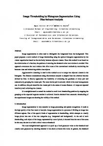
Where, is the level set function, is the speed function, which drives and attracts the active contour towards the region boundaries. The second term of the right hand represents the curvature, which is used to smooth the contour. It is nonlinear and computational expansive α and β user-controlling parameters. For solving the LSE, most classical methods such as the upwind scheme are based on some finite difference, finite volume or finite element approximations and an explicit computation of the curvature [13]. These methods requires a lot of CPU time. Recently, the lattice Boltzmann method (LBM) has been used as solver for accelerating the PDE (partial differential equation) [12]. The LBM at first designed to simulate Navier-Stokes equations for an incompressible fluid [26]. Figure 1 illustrated the D2Q5 (two dimensions and five lattice speeds)LBM lattice structure.
Fig.1. Spatial Structure of D2Q5 LBM Lattice
The evolution equation of LBM is
5
(⃗
)
⃗⃗⃗⃗ ,
(⃗ )
(⃗ )
(2)
(3)
⃗⃗⃗⃗ ⃗
( ⃗ )-
To model the typical diffusion phenomenon, the following local equilibrium particle distribution is to be used [27-28],
( )
with
(4)
3 Designed Level Set Method In general, Level Set Methods could be categorized into two major classes’ namely region-based methods and edge-based methods. In region-based models each region of interest is identified using a region descriptor to guide the motion of the active contour [29-30]. In this section, the conception of the proposed fast convex level set algorithm is described in detail. In the current work, energy functional has been designed for minimization is as ( ) Where rameters.
( )
( )
(5)
( )
the set isfunction level, while and
are the positive controlling pa-
( )
A. Design of
( ) is the histogram based link with the image data, The energy term which defined as follows: ( )
(
)
* (
)+
(6)
Here, H is the Heaviside function; Im is the mean value and is level set function which is defined as the signed distance function [13]. The mean values and are defined as: (
) ( )
(7)
( ) (
)( (
With
( )) ( ))
(8)
6
B. Design of
( )
The energy term is texture based, which is defined as follows with the image domain[25], where and are the inside and outside evolving curve of the image domain; respectively. The energy term is given by: ( )
(
, (
)
)
)-
( )(
(
(9)
)
Where, H is the Heaviside function.
( )
B. Design of
The regularization term used as a constraint on the evolving contour, can be expressed as: ( ) | ( )| (10) Therefore, the proposed energy functional in equation (5) can be rewritten as: (
( ) )) ( )
( (
(
) ( ) ))(
( ( ))
)(
( )) ( )
(
(11) Using the gradient descent method, the level set equation can be recovered from the above defined energy functional
⁄ Where
⁄
(12)
⁄
is the Gateaux derivative of . ⁄
(
( ),(
(
(
))
))
⁄
(
* (
))
) (13)
The gradient projection method allowed replacing φ is a signed distance function (SDF), thus | φ| = 1.
by | φ|. In addition, since
The body force F can be expressed as: (
)
* (
))
(
(
))
(14)
7
Where, and are the controlling parameters used to adjust the impact of F on the active contour motion. The principal implementation steps of the proposed method are provided in the following algorithm. _______________________________________________________ Algorithm: Level set methods for image segmentation with LBM _______________________________________________________ Start Initialize the distance function signed distance function Compute the body force F in equation (14) Resolve the LSE using LBM Accumulate ( ⃗ ) the values at each grid point which generates updated values and find the contour Check convergence Ifthe evolving curve has not converged go back to step Else End End ______________________________________________________
4
Experimental Results and Analysis
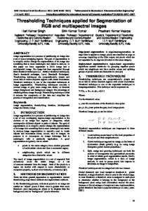
Several experiments were carried out using various kinds of images in order to demonstrate the performance of the proposed method. Figure 2 demonstrated sample of the tested images, where the original images in (a), while (b) the segmented images and (c) the gray representation for the segmented images.
Image (2.1)
Image (2.2)
Image (2.3)
8
(a)
(b)
(c)
Fig. 2.Segmentation of different images (a) represent original images, (b) represent the evolution of the contour and (c) represents result of proposed method.
To evaluate the performance of the proposed method, the Dice’s coefficient and Jaccards’ coefficient measures set agreement was calculated. The Dice’s coefficient is one of the measurementsto measure the extent of spatial overlap between the two binary images. This coefficient is commonly used in reporting the performance of segmentation. A value of 0 indicates no overlap, while a value of 1 indicates perfect agreement (similarity). Higher numbers indicate better agreement. Table 1 demonstrated comparing the designed method to Li method [14] in terms of the Dice’s coefficient values.
Image index
Table 1 Dice’s coefficient (D) Proposed method Li method [14]
Image2.1
0.94
0.53
Image 2.2
0.92
0.22
Image2.3
0.89
0.42
Average
0.92
0.39
9
It is established from Table 1 that the proposed method is outperformed Li method in terms of the Dice’s coefficient values for all compared images. The average value of agreement achieved by the designed method is 0.92. The special overlap between the pair of segmentations can be measured by using Jaccards coefficient. Table 2 Jaccard’coefficient (D) Image index Proposed method Li method[14] Image 2.1
0.84
0.28
Image 2.2
0.73
0.39
Image 2.3
0.79
0.26
Average
0.78
0.31
It is established from Table 2 that the designed method is outperformed Li method in terms of the Jaccards ‘coefficient values for all compared images. The average value of agreement achieved by the designed method is 0.78. Comparing both algorithms with respect to the computational time was conducted in Table 3. Table 3 Total time taken to run the algorithm in seconds Image index Proposed method Li method[14] Image 2.1
1.54
92.65
Image 2.2
1.28
82.527
Image 2.3
1.23
76.72
Average
1.35
83.97
Table 3 proved that the proposed method is superior to Li method in terms of the computational time taken to run the segmentation process. The proposed method has been taken 1.35 seconds, while running Li method has been taken 83.97 seconds. Researchers are interested with different image and signal processing applications [31-33]. In the current work, the preceding results established that the proposed segmentation methods using Level set methods for image segmentation achieved 0.92 average similarity value and average 1.35 seconds to run the algorithm. The results established that the proposed method is outperformed the segmentation method using Li method for segmentation.
10
5 Conclusion The current work proposed a histogram and thresholding based level set model. The use of the lattice Boltzmann method to solve the level set equation enables the algorithm to be highly parallelizable. The designedmethod is effective for segmenting objects with and without edges. Experimental results of different kinds of real images have been demonstrated the effectiveness of the designed model. The proposed method achieved 0.92 average similarity value with average 1.35 seconds running time, which outperform Li method in [14] that used the level set method for image segmentation.
References [1] N. Dey, A. B. Roy, M. Pal and A. Das, ”FCM Based Blood Vessel Segmentation Method For Retinal Images,” International Journal of Computer Science and Network, Vol. 1, No. 3, 2012. [2] S. Samanta, N. Dey, P. Das, S. Acharjee and S. S. Chaudhuri, “Multilevel Threshold Based Gray Scale Image Segmentation using Cuckoo Search,” International Conference on Emerging Trends in Electrical, Communication And Information Technologies -ICECIT, Dec 12-23, 2012. [3] S. Samanta, S. Acharjee, A. Mukherjee, D. Das and N. Dey, “Ant Weight Lifting Algorithm for Image Segmentation”, 2013 IEEE International Conference on Computational Intelligence and Computing Research, Madurai, Dec 26-28 2013. [4] S. Bose, A. Mukherjee, Madhulika, S. Chakraborty, S. Samanta and N. Dey, “Parallel Image Segmentation using Multi-Threading and K-Means Algorithm,” 2013 IEEE International Conference on Computational Intelligence and Computing Research, Madurai, Dec 26-28 2013. [5] P. Roy, S. Chakraborty, N. Dey, G. Dey, R. Ray and S. Dutta, “Adaptive Thresholding: A comparative study,” International Conference on Control, Instrumentation, Communication and Computational Technologies-2014, 10-11 July 2014. [6] P. Roy, S. Goswami, S. Chakraborty, A. T. Azar and N. Dey, “Image Segmentation using Rough Set theory: A Review,” International Journal of Rough Sets and Data Analysis, Vol. 1, No. 2, pp.62-74, 2014. [7] G. Pal, S. Acharjee, D. Rudrapaul, A. S. Ashour and N. Dey, Video Segmentation using Minimum Ratio Similarity Measurement, International Journal of Image Mining, Vol. 1, No. 1, 2015. [8] R. C. Gonzalez and R. E. Woods, Digital Image Processing. Addison-Wesley Publishing Company, 1993. [9] Z. Chi, H. Yan, T. Pham, Fuzzy Algorithms: with applications to images processing and pattern recognition. Word Scientific, 1996. [10] N. Otsu, “A threshold selection method from gray-level histograms”, IEEE Trans. Systems, Man, and Cybernetics, vol. SMC-9, no. 1, pp. 62-66, 1979.
11 [11] J. Kittler and J. Illingworth, “Minimum error thresholding”, Pattern Recognition, vol. 19, pp. 41-47, 1986. [12] O. J. Tobias and R. Seara, “Image segmentation by histogram thresholding using fuzzy sets”, IEEE Trans. On Image Processing, vol. 11, pp. 1457-1465, 2002. [13] S. Balla-Arabe, X. Gao and B. Wang, “GPU Accelerated Edge-Region Based Level Set Evolution Constrained By 2D Gray-scale Histogram,”IEEE Transactions on Image Processing, Vol. 10, No. 1, 2013, pp. 1-11. [14] C. Li, R. Huang, Z. Ding, J. Chris, D. N. Metaxas, and J.C. Gore, “A level set method for image segmentation in the presence of intensity inhomogeneities with application to MRI,” IEEE Trans. Image Process., Vol. 20, No. 7,July2011, pp. 2007–2016 [15] T. Chan and L. Vese, “Active contours without edges,” IEEE Trans. Image Processing, Vol. 10, No. 2, Feb. 2001,pp. 266– 277. [16] K. Zhang, L. Zhang, H. Song, and W. Zhou, “Active contours with selective local or global segmentation: A new formulation and level set method,” Image Vis. Comput., Vol. 28, No. 4, Apr. 2010, pp. 668–676. [17] S. Balla-Arabé, B. Wang, and X.-B. Gao, “Level set region based image segmentation using lattice Boltzmann method,” In Proc. 7th Int. Conf. Comput. Intell. Security, Dec. 2011, pp. 1159–1163. [18] S. Balla-Arabé and X. Gao, “A multiphase entropy-based level set algorithm for MR breast image segmentation using lattice boltzmann model,” In Proc. Sino, Foreign, Interchange Workshop Intell. Sci. Intell. Data Eng., Oct. 2013, pp. 8–16. [19] Lie, I., Beschiu, C., Nanu, S. FPGA Based Signal Processing Structures,Saci 2011 6th IEEE International Symposium on Applied Computtional Intelligence and Informatics, Proceedings, 5873043, pp. 439-444. [20] NanuSorin, Lie Ioan, Belgiu George, MusuroiSorin, High Speed Digital Controller Implemented with FPGA, BuletinulStiintific al UPT, seria Electronica siTelecomunicatii, 2010, vol55(69), pag.17-22. [21] Belgiu, G., Nanu, S., Silea, I. Arificial Intelligence in Machine Tools Design Based on Genetic Algorithms Application, Sofa 2010 - 4th International Workshop on Soft Computing Applications, Proceedings, 5565623, pp. 57-60 [22] S. Balla-Arabé, X. Gao, and B.Wang, “A fast and robust level set method for image segmentation using fuzzy clustering and lattice Boltzmann method,” IEEE Trans. Syst. Man, Cybern. Part B, Cybern. Vol. 99, 2012, pp. 1–11. [23] R. TsaiI and S. Osher, “Level Set Methods And Their Applications In Image Science,” Communication Mathematical Science, Vol. 1, No. 4, 2003, pp. 1-20. [24] S. Balla-Arabe and XinboGao, “Image multi thresholding by combining the lattice Boltzman model and localized level set algorithm,” Neurocomputing, Vol. 93, 2012, pp. 106-114. [25] S. Balla-Arabé1, XinboGao and Lai Xu, “Texture-Aware Fast Global Level Set Evolution,” 2014. [26] S. Balla-Arabe and XinboGao, “Geometric active curve for selective entropy optimization,” Neurocomputing, Vol. 139, 2014, pp. 65-76. [27] M Y. Zhao, “Lattice Boltzmann based PDE solver on the GPU,” Vis. Comput., Vol. 24, No. 5, May 2007, pp. 323–333. [28] P. Bhatnager, E. Gross and M.Krook, Phys. Rev. 94, 511 (1954).
12 [29] C. Li, C. Xu, C. Gui and M. Fox: Distance regularized level set evolution and its application to image segmentation,” IEEE Transactions on Image Processing, Vol. 19, No. 12, 2010, pp. 3243-3254. [30] S. Osher and R. Fedkiw, Level Set Methods and Dynamic Implicit Surfaces, New York, Springer-Verlag, 2003. [31] V. K. Sudha, R. Sudhakar and V. E. Balas, “Fuzzy rule-based segmentation of CT brain images of hemorrhage for compression,” International Journal of Advanced Intelligence Paradigms, Vol. 4, pp. 256-267, 2012. [32] S. Senthilkumar and A. R. M. Piah, “An improved fuzzy cellular neural network (IFCNN) for an edge detection based on parallel RK (5, 6) approach,” International Journal of Computational Systems Engineering, Vol.1, No.1, pp. 70-78, 2012. [33] S. Bharathi, R. Sudhakar and V. E. Balas, “Biometric recognition using fuzzy score level fusion,” International Journal of Advanced Intelligence Paradigms, Vol. 6, No.2, pp. 81-94, 2014.