Improved Algorithms and Hardware Designs for Division by ...

Copyright by Inwook Kong 2009

The Dissertation Committee for Inwook Kong certifies that this is the approved version of the following dissertation:

Improved Algorithms and Hardware Designs for Division by Convergence

Committee:

Earl E. Swartzlander, Jr., Supervisor Anthony P. Ambler Mircea D. Driga Mohamed G. Gouda Nur A. Touba

Improved Algorithms and Hardware Designs for Division by Convergence

by Inwook Kong, B.S.E.E., M.E.E.E.

DISSERTATION Presented to the Faculty of the Graduate School of The University of Texas at Austin in Partial Fulfillment of the Requirements for the Degree of DOCTOR OF PHILOSOPHY

THE UNIVERSITY OF TEXAS AT AUSTIN December 2009

Dedicated to my wife, Youngsook Park, for her love and support.

Acknowledgments

I wish to thank all the people who have helped me accomplish this research. This research would not be possible without their help and support. First of all, I would like to thank my supervisor, Dr. Earl E. Swartzlander, Jr. for his invaluable guidance, support, and expertise in this field. He has guided me throughout my research with remarkable insight and profound knowledge. Without his guidance and support, this research could not have been achieved. I am also grateful to the members of my dissertation committee, Dr. Anthony P. Ambler, Dr. Mircea D. Driga, Dr. Mohamed G. Gouda, and Dr. Nur A. Touba. Their helpful advices on my research and their knowledge have guided me in my quest to do quality work. I would like to thank my friends in Austin and the colleagues in the application specific processor group for their help and cheering up. I am also indebted to many people in Samsung for their support and concern for me. Finally, I would like to thank my wife Youngsook Park, who always supports and encourages me with great love, my daughter Junghyun, who always cheers me up, and my parents and parents-in-law for their love throughout my life.

v

Improved Algorithms and Hardware Designs for Division by Convergence Publication No. Inwook Kong, Ph.D. The University of Texas at Austin, 2009 Supervisor: Earl E. Swartzlander, Jr.

This dissertation focuses on improving the division-by-convergence algorithm. While the division by convergence algorithm has many advantages, it has some drawbacks, such as a need for extra bits in the multiplier and a large ROM table for the initial approximation. To mitigate these problems, two new methods are proposed here. In addition, the research scope is extended to seek an efficient architecture for implementing a divider with Quantum-dot Cellular Automata (QCA), an emerging technology. For the first proposed approach, a new rounding method to reduce the required precision of the multiplier for division by convergence is presented. It allows twice the error tolerance of conventional methods and inclusive error bounds. The proposed method further reduces the required precision of the multiplier by considering the asymmetric error bounds of Goldschmidt dividers. vi

The second proposed approach is a method to increase the speed of convergence for Goldschmidt division using simple logic circuits. The proposed method achieves nearly cubic convergence. It reduces the logic complexity and delay by using an approximate squarer with a simple logic implementation and a redundant binary Booth recoder. Finally, a new architecture for division-by-convergence in QCA is proposed. State machines for QCA often have synchronization problems due to the long wire delays. To resolve this problem, a data tag method is proposed. It also increases the throughput significantly since multiple division computations can be performed in a time skewed manner using one iterative divider.

vii

Table of Contents

Acknowledgments

v

Abstract

vi

List of Tables

xi

List of Figures

xii

Chapter 1. Introduction 1.1 Background and Motivation . . . . . . . . . . . . . . . . . . . 1.2 Research Direction . . . . . . . . . . . . . . . . . . . . . . . . 1.3 Dissertation Organization . . . . . . . . . . . . . . . . . . . . . Chapter 2. Division by Convergence 2.1 Goldschmidt Division . . . . . . . . . . . . . . . . . . . . . . . 2.2 Previous Works . . . . . . . . . . . . . . . . . . . . . . . . . . 2.2.1 Rounding Methods for Division by Convergence . . . . . 2.2.2 Reduction of the Required Multiplier Precision . . . . . 2.2.3 Computation Time Reduction of Division by Convergence A New Rounding Method with Improved Error Tolerance 3.1 Overview . . . . . . . . . . . . . . . . . . . . . . . . . . . . . . 3.2 Current Rounding Method . . . . . . . . . . . . . . . . . . . . 3.3 New Rounding Method . . . . . . . . . . . . . . . . . . . . . . 3.3.1 Inclusive Error Bounds . . . . . . . . . . . . . . . . . . 3.3.2 Twice the Error Bounds with Inclusive Endpoints . . . . 3.3.3 Extension for Asymmetric Error Bounds . . . . . . . . . 3.3.4 Details of the New Rounding Method . . . . . . . . . .

1 1 3 5 7 7 10 10 12 12

Chapter 3.

viii

15 15 16 19 19 21 23 26

3.4 Approximation Error Bounds of Goldschmidt Dividers . . . . . 3.4.1 Goldschmidt Divider . . . . . . . . . . . . . . . . . . . . 3.4.2 Error Bounds for the Goldschmidt Divider . . . . . . . . 3.4.3 Error Bounds Comparison by the Fi Computation Methods 3.4.4 Parameters for the New Rounding Method . . . . . . . 3.4.5 Comparison with Other Methods . . . . . . . . . . . . . 3.5 Verification and Simulation Results . . . . . . . . . . . . . . . 3.5.1 Implementation and Verification . . . . . . . . . . . . . 3.5.2 Simulation Results . . . . . . . . . . . . . . . . . . . . . 3.6 Summary . . . . . . . . . . . . . . . . . . . . . . . . . . . . . . Chapter 4. Division with Faster than Quadratic Convergence 4.1 Overview . . . . . . . . . . . . . . . . . . . . . . . . . . . . . . 4.2 Division with Faster Convergence . . . . . . . . . . . . . . . . 4.2.1 Quadratic Convergence . . . . . . . . . . . . . . . . . . 4.2.2 Division with Faster Convergence . . . . . . . . . . . . . 4.3 The DFQC Method . . . . . . . . . . . . . . . . . . . . . . . . 4.3.1 Division Method with Faster than Quadratic Convergence 4.3.2 Performance Analysis of the DFQC Method . . . . . . . 4.4 Implementation Details of the DFQC Method . . . . . . . . . 4.4.1 Squarer . . . . . . . . . . . . . . . . . . . . . . . . . . . 4.4.2 Limitation of the DFQC Method in Radix-4 Multiplier . 4.4.3 Radix-8 Redundant Binary Booth Recoder for CarrySave Representation . . . . . . . . . . . . . . . . . . . . 4.4.4 Special RBBRs to interface with NBBRs . . . . . . . . . 4.5 Simulation and Results . . . . . . . . . . . . . . . . . . . . . . 4.5.1 Simulation Environment . . . . . . . . . . . . . . . . . . 4.5.2 Implementation of an Example Goldschmidt Divider . . 4.5.3 Simulation for the DFQC Performance Analysis . . . . . 4.5.4 Verification of Division by the DFQC Method . . . . . . 4.5.5 Delay for the DFQC Method . . . . . . . . . . . . . . . 4.5.6 Area of the DFQC Method . . . . . . . . . . . . . . . . 4.6 Summary . . . . . . . . . . . . . . . . . . . . . . . . . . . . . . ix

27 27 28 32 33 34 35 35 37 38 40 40 41 42 42 45 45 48 53 53 54 55 57 59 59 59 61 63 64 66 68

Chapter 5. 5.1 5.2

5.3

5.4

5.5 5.6

Goldschmidt Iterative Divider for Quantum-dot Cellular Automata Overview . . . . . . . . . . . . . . . . . . . . . . . . . . . . . . Quantum-dot Cellular Automata . . . . . . . . . . . . . . . . . 5.2.1 QCA Cell . . . . . . . . . . . . . . . . . . . . . . . . . . 5.2.2 Logic Gates in QCA . . . . . . . . . . . . . . . . . . . . 5.2.3 Clock Zones . . . . . . . . . . . . . . . . . . . . . . . . 5.2.4 Coplanar Wire Crossing . . . . . . . . . . . . . . . . . . 5.2.5 Conventional Goldschmidt Divider Architecture in QCA Data Tag Method for Iterative Computation . . . . . . . . . . 5.3.1 Problems in Using State Machines for QCA . . . . . . . 5.3.2 Data Tag Method . . . . . . . . . . . . . . . . . . . . . 5.3.3 Goldschmidt Divider with the Data Tag Method . . . . Details of Implementation . . . . . . . . . . . . . . . . . . . . 5.4.1 Design Guidelines for Robust QCA Circuits . . . . . . . 5.4.2 Implementation of Goldschmidt Divider . . . . . . . . . 5.4.2.1 Tag Generator . . . . . . . . . . . . . . . . . . 5.4.2.2 Tag Decoder and Multiplexers for {Di , Ni } . . . 5.4.2.3 Multiplexers for Fi . . . . . . . . . . . . . . . . 5.4.2.4 23 × 3-bit ROM Table . . . . . . . . . . . . . . 5.4.2.5 12-bit Array Multiplier . . . . . . . . . . . . . . Simulation Results . . . . . . . . . . . . . . . . . . . . . . . . Summary . . . . . . . . . . . . . . . . . . . . . . . . . . . . . .

Chapter 6. Conclusions 6.1 Conclusions . . . . 6.2 Published Results . 6.3 Future Work . . . .

and . . . . . . . . .

Future Work . . . . . . . . . . . . . . . . . . . . . . . . . . . . . . . . . . . . . . . . . . . . . . . . . . . . . . . . . . . . . . .

Bibliography

70 70 71 71 72 74 75 76 77 77 77 79 81 81 81 82 82 84 84 88 89 92 94 94 96 96 98

Vita

106

x

List of Tables

3.1 3.2

Conventional method rounding rule details . . . . . . . . . . . New rounding rules . . . . . . . . . . . . . . . . . . . . . . . .

3.3 3.4

3.6

Conversion from QA to QT . . . . . . . . . . . . . . . . . . . . Maximum error bounds of the approximate quotient for the Goldschmidt divider as implemented . . . . . . . . . . . . . . Maximum error bounds of the approximate quotient when Fi is computed by a two’s complement operation . . . . . . . . . . Required extra bits for each rounding method . . . . . . . . .

3.7

Maximum error bounds of E during the simulation . . . . . .

38

4.1 4.2

52

4.5

Maximum errors of the conventional and the DFQC method . Maximum approximation errors of the final quotients during the simulation . . . . . . . . . . . . . . . . . . . . . . . . . . . Critical path delays for the DFQC method and a 3X adder . . Initial errors and the required table sizes for double precision floating-point . . . . . . . . . . . . . . . . . . . . . . . . . . . Area costs of the DFQC method and the quadratic method . .

5.1 5.2

Throughput of the divider using the data tag method . . . . . Delays of the functional units in the Goldschmidt divider . . .

3.5

4.3 4.4

′′

′′

xi

19 23 26 30 31 35

64 65 66 67 80 92

List of Figures

2.1

Block diagram of a typical Goldschmidt divider. . . . . . . . .

9

3.1 3.2

QA , Q, and QT in the conventional rounding method. . . . . . RI rounding mode with inclusive error bounds. . . . . . . . . .

18 20

3.3

Q, QA , and QT in the new rounding method. . . . . . . . . . .

3.4 3.5 3.6 3.7 4.1

′′

22

′′

Q, QA , and QT in the new rounding method for unidirectional errors. . . . . . . . . . . . . . . . . . . . . . . . . . . . . . . . Histogram of E for 109 random divisions. . . . . . . . . . . . . Goldschmidt divider and verification environment. . . . . . . . ′′ Histogram of E by 1010 random input vectors. . . . . . . . .

25 32 35 37

A floating-point Goldschmidt divider implemented using the DFQC method with two squaring units. . . . . . . . . . . . .

46

′

4.2 4.3 4.4 4.5

Fi computation using m × m squaring for near cubic convergence. Modified radix-8 carry-save Booth recoder. . . . . . . . . . . . 4-bit squarer and radix-8 redundant binary Booth recoders. . . Error histograms of the DFQC method and the quadratic convergence. . . . . . . . . . . . . . . . . . . . . . . . . . . . . . .

47 56 57

5.1 5.2 5.3 5.4 5.5 5.6 5.7 5.8 5.9 5.10

Basic QCA cells with two possible polarizations. . . . . . . . . Layout and schematic symbol of a conventional inverter in QCA. Layout of various inverters in QCA. . . . . . . . . . . . . . . . Layout and schematic symbol of a majority gate in QCA. . . . QCA clock signals for four clock zones. . . . . . . . . . . . . . QCA wire with clock zones. . . . . . . . . . . . . . . . . . . . Layout of an example for coplanar wire crossovers. . . . . . . . Goldschmidt divider block diagram for CMOS. . . . . . . . . . Computation unit implementations using a state machine. . . Computation unit implementations using the data tag method.

71 72 73 74 75 75 76 77 78 78

xii

62

5.11 Block diagram of the Goldschmidt divider with the data tag method. . . . . . . . . . . . . . . . . . . . . . . . . . . . . . . 5.12 Schematic and layout of the tag generator. . . . . . . . . . . . 5.13 Tag decoder for multiplexers for {Di , Ni }. . . . . . . . . . . . 5.14 Tag decoder for multiplexers and latches for Fi . . . . . . . . . 5.15 Layout of the 3-bit reciprocal ROM. . . . . . . . . . . . . . . . 5.16 Layout of a cell for the array multiplier. . . . . . . . . . . . . 5.17 Schematic of a 4×4-bit multiplier using the multiplier cell. . . 5.18 Layout of the Goldschmidt divider with a 12-bit multiplier. . . 5.19 Simulation results of the implemented divider. . . . . . . . . .

xiii

80 83 85 86 87 88 89 90 91

Chapter 1 Introduction

1.1

Background and Motivation Division is a basic operation in many scientific and engineering ap-

plications, and two categories of division algorithms have been developed by researchers. Although division is typically an infrequent operation compared to addition and multiplication, it has been shown that if division is ignored, many applications will experience performance degradation [1]. Division algorithms can be categorized into two kinds: digit recurrent division and division by convergence. While these two kinds of algorithms have their own advantages [2], division by convergence has several advantages, such as quadratic convergence, a pipeline friendly algorithm, and a small size if the system includes a multiplier [3]. Goldschmidt division [2, 4] is a representative algorithm for the hardware implementations of division by convergence. While division by convergence algorithms have some advantages, such as quadratic convergence and small size if the system includes a multiplier [3], they have several drawbacks. First, they do not provide an exact remainder that is necessary for correct rounding. In addition, they require extra bits in the multiplier for a correctly rounded quotient and the mitigation of the trun-

1

cation errors. Due to these extra bits, the precision of the multiplier should be larger than the required target precision. Second, the computation time of division by convergence heavily depends on the precision of the initial approximation to the reciprocal of denominator. Typically, the initial approximation is computed using a table look-up method, and the accuracy of the initial approximation determines the number of iterations to obtain a target precision. Although a high precision initial reciprocal table can reduce the number of iterations, it requires a large silicon area. If these drawbacks can be mitigated, the performance of the division by convergence algorithms will be improved. In addition to improving algorithms for division by convergence in CMOS technology, a new architecture for a promising emerging nanotechnology also needs to be explored. The continued scale down of transistors confronts many challenges, such as leakage current caused by quantum mechanical tunneling of electrons. Quantum-dot Cellular Automata (QCA) [5, 6] is one of the promising emerging nanotechnologies, which may solve the problems due to the shrink of transistors. QCA has many advantages, such as low power consumption, high density, ultra fast computing, and an inherent pipeline structure by implicit D flip-flops. Due to the unique characteristics of the QCA technology, many arithmetic circuits, such as adders and multipliers, show interesting performance characteristics in the QCA technology [7, 8]. It means that an arithmetic algorithm that shows the best performance in the CMOS technology may not be the best in the QCA technology. Therefore, new arithmetic algorithms specialized for the QCA technology need to

2

be developed.

1.2

Research Direction Although division by convergence has many advantages, it requires ex-

tra bits for a multiplier (more than the target precision) and a large silicon area for a high precision initial reciprocal approximation. In addition, a new architecture for an emerging nanotechnology, quantum-dot cellular automata, needs to be developed. To improve the division by convergence algorithm, three approaches are proposed in this dissertation. The approximate quotients have to be computed with extra precision due to both truncation errors during iterations and IEEE-754 compliant rounding operations. The truncation error occurs on every iteration since multiplication results are rounded to the precision of the multiplier. The final approximate quotient always has a bounded small error due to these truncation errors. Another reason for the extra precision requirement is IEEE-754 compliant rounding. The conventional rounding method [3, 9–11] requires that the total error of the final approximate quotient should be less than 14 ulp. In other words, the number of extra bits in the multiplier has to be large enough so that the total error of the final approximate quotient is less than 41 ulp. In order to reduce the required extra precision for the approximate quotient, a new rounding method for division by convergence is proposed. The proposed rounding method applies special truncation methods at the final iteration step. This requires a minor modification to the rounding constants of the multiplier. 3

It allows twice the error tolerance of conventional methods and inclusive error bounds. The proposed method further reduces the required precision of the multiplier by considering the asymmetric error bounds of Goldschmidt dividers where the factors are computed using a one’s complement operations. Since the accuracy of the initial reciprocal approximation determines the number of iterations in division by convergence, an efficient reciprocal approximation method is crucial to reduce the computation time. Although a reciprocal ROM table with large precision reduces the number of iterations, it also requires a large silicon area. Therefore, many researchers have focused on implementations of efficient reciprocal approximation methods. In contrast, if the rate of convergence becomes higher than quadratic in division by convergence, the accuracy requirement for an initial reciprocal approximation can be mitigated. In other words, the target precision of a final approximate quotient can be computed from a less accurate reciprocal approximation if the speed of convergence is faster. In order to reduce the silicon area for the ROM table, a new method to speed the convergence rate using near cubic convergence is proposed. Although division with cubic convergence, the simplest higher order convergence, has been regarded as impractical due to its complexity, the new method reduces the logic complexity and delay by using an approximate squarer with a simple logic implementation and a redundant binary Booth recoder. Although Quantum-dot Cellular Automata (QCA) [5, 6] has many advantages, there is a problem in implementing conventional sequential circuits 4

based on state machines. Wires in QCA have a long delay since they are implemented by QCA cells like those used to construct gates. Therefore, state machines for QCA often have synchronization problems due to the long delays between the state machines and the units (i.e., the computational circuits) to be controlled. Due to this difficulty in designing sequential circuits, it appears that a division circuit has not been researched yet while many adders and multipliers have been designed in QCA [7, 8, 12–15]. To resolve this problem, an architecture for division by convergence using a data tag method is proposed. In the new architecture for QCA, data tags are used instead of state machines, and they are associated with the data and local tag decoders generate control signals. Since each datum has a tag in the new architecture, it is possible to issue a new division command at any iteration stage of a previous issued operation, which increases the throughput of division significantly.

1.3

Dissertation Organization The proposed research focuses on improving the division by conver-

gence algorithms. The rest of this dissertation is organized as a total of five chapters. In Chapter 2, the conventional algorithm for division by convergence is explained with its detailed operation. In addition, the previous works to mitigate the drawbacks of division by convergence are summarized. As the first approach, a new rounding method to reduce the required multiplier precision for division by convergence is presented in Chapter 3. In Chapter 4, an approach to increase the speed of convergence for Goldschmidt division using

5

simple logic circuits is presented. In Chapter 5, an architecture for division by convergence in QCA is presented Finally, the summary of the research work in this dissertation and suggestions for the future research are provided in Chapter 6.

6

Chapter 2 Division by Convergence

The concept of division by convergence and its previous researches are shown in this chapter. In Section 2.1, the concept of Goldschmidt division is explained. Goldschmidt division is a representative division-by-convergence algorithm that is usually used for hardware implementations. In the other sections, previous researches to solve the problems shown in Section 1.2 are reviewed.

2.1

Goldschmidt Division In this section, the concept of Goldschmidt division and its implemen-

tation are explained. The division-by-convergence algorithms explored in this dissertation are various forms of Goldschmidt division, sometimes called a series expansion method [10]. Goldschmidt dividers compute the approximate quotient by parallel multiplications. Division can be written as Q=

N D

where Q is the quotient, N is the numerator, and D is the denominator. Before the first iteration of the Goldschmidt division, both N and D are multiplied by F0 (the approximate reciprocal of D) to make the denominator close to 7

1. Since F0 is produced by a reciprocal table with a limited precision, the resulting denominator has an error, ǫ. Therefore, the normalized quotient, Q0 , is Q0 =

N × F0 N0 N0 = = . D × F0 D0 1−ǫ

At the first Goldschmidt iteration, N0 and D0 are multiplied by F1 . While F0 is usually computed by a table look-up, the approximation for the reciprocal of D0 , F1 , is computed by an addition. This simple arithmetic computation for the approximate reciprocal is one of the advantages of Goldschmidt division. In this case, F1 and Q1 are computed as follows: F1 = (2 − D0 ) = 1 + ǫ N0 × F1 N1 = D1 D0 × F1 N0 (1 + ǫ) N0 (1 + ǫ) = = (1 − ǫ)(1 + ǫ) (1 − ǫ2 )

Q1 =

At the i-th iteration, Fi and Qi are computed as follows: i−1

Fi = (2 − Di−1 ) = 1 + ǫ2

for i > 0

(2.1)

2i−1

Qi =

Ni Ni−1 × Fi Ni−1 (1 + ǫ ) = = Di Di−1 × Fi (1 − ǫ2i )

(2.2)

As the iteration continues, Ni will converge toward Q with ever-greater precii

sion. Since the error decreases by ǫ2 as shown in Equation (2.2), the convergence order of the Goldschmidt division is quadratic. A less than 8-bit reciprocal table [16] can make the initial error ǫ accurate enough for double precision floating-point division to be computed in three Goldschmidt iterations. In addition, the Goldschmidt division is attractive for hardware implementation 8

since the independent parallel multiplications can be implemented efficiently in a pipelined multiplier. Fi for quadratic convergence is usually computed using simple logic without a real addition. If the two’s complement operation used to compute Fi in Equation (2.1), it requires a carry propagating adder, which introduces a long delay. Therefore, Fi is usually computed by one’s complement [3, 17] to reduce the delay although one’s complement introduces a small error, 2−lsb, as

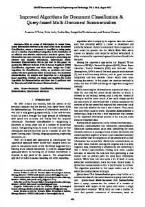
Unpack N

D FF

2-D

Table

FF

MUX

MUX

MUX Rounding constatnts &N

Multiplier Round Q T,R

Exponent

Round & Normalization Pack

Figure 2.1: Block diagram of a typical Goldschmidt divider.

9

follows: Fi = 2 − Di−1 = comp2(Di−1 ) = comp1(Di−1 ) + 2−lsb ≈ comp1(Di−1 )

(2.3)

Since Fi can be computed by one’s complement, many Goldschmidt division applications have adopted the quadratic convergence algorithm. A typical floating point Goldschmidt divider consists of a multiplier, a reciprocal table, a computation unit for Fi , and rounding unit as shown in Figure 2.1.

2.2 2.2.1

Previous Works Rounding Methods for Division by Convergence Since a correction stage to compute the exact remainder is required

for correct rounding in division-by-convergence, several efficient methods have been suggested for the IEEE-754 compliant rounding. The first approach is to use more than twice the precision for intermediate computation [18]. A method using a double precision accumulator was suggested to compute correctly rounded results of the Newton-Raphson iterations in the IBM RS/6000 processor [19], but the method has two drawbacks. One is that the accumulator for a multiply-and-add instruction requires twice the precision of other methods. The other is that the method needs one additional regular iteration step before the final rounding stage although the result has already reached the target precision. However, the method is very efficient for the fused multiply10

and-add architecture, and it utilizes the floating-point pipeline architecture successfully without any conditional branches for the rounding stage. Another approach is to compute the direction of the remainder in lieu of an explicit calculation. Because this method requires only the direction of the remainder for the rounding operation, more efficient rounding circuits can be implemented. A method that computes the sign of the difference between the dividend and the product of an approximate quotient and the divisor was implemented in the TI-8847 processor [2, 20]. In this processor, quotients are computed with extra bits of precision. An enhanced method that removes the necessity of comparing the remainder in some cases using one additional correct bit [9] was developed. Furthermore, it has been shown that a reduction in the frequency of remainder comparisons is possible if several additional bits are computed [10, 21]. Although there have been improvements in the frequency of the remainder comparisons, the error tolerance of inputs to the rounding stage has not improved. Truncation of the numerator and denominator in division by convergence introduces a small amount of error at each iteration step. In the Goldschmidt division algorithm [4], this kind of error accumulates, and the total error for the approximate quotient is proportional to the number of iterations. For correct operation at the rounding stage, the absolute value of the total error has to be less than ± 14 ulp in current rounding methods. If this error tolerance can be increased, the intermediate precision required for iterations can be relaxed, or an iteration algorithm can be implemented with more error 11

margin. 2.2.2

Reduction of the Required Multiplier Precision Goldschmidt division requires a high precision multiplier due to the

extra bits required for correct rounding. To reduce the multiplier precision, several approaches have been suggested. One approach is to determine the required minimum extra bits of the multiplier by error analysis. For the AMD K-7 microprocessor, 7 extra bits were used for a 2-iteration 68-bit division after a conservative error analysis [3]. Tighter error analyses show that the required number of extra bits can be reduced further [22, 23]. Another recent approach to reduce the required multiplier precision is a method using a rectangular m × n multiplier [11], which uses a property of Goldschmidt division that the multiplicative factors are close to 1. 2.2.3

Computation Time Reduction of Division by Convergence Many researchers have tried to reduce the computation time of division

by convergence, and the most prevalent approach is to reduce the number of iterations by increasing the precision of the initial approximation to the reciprocal. It is used to compute the initial quotient value in Goldschmidt division. The number of iterations and the computation time are heavily dependent on the accuracy of the initial reciprocal approximation. Although a high precision initial reciprocal table can reduce the number of iterations, it requires a large silicon area.

12

Several methods have been suggested to increase the accuracy of the reciprocal approximation. The efficient implementation of the reciprocal approximation is crucial for the performance of division by convergence. Although the minimum size of the reciprocal ROM table with a certain error margin can be determined [16], a naive implementation still requires a large silicon area. One approach to reduce the area for the reciprocal table is the faithful bipartite ROM reciprocal table method [24, 25], which employs two independent parallel table look-ups and then adds the output values of the two tables to compute the final value. Since the addition can be computed at the Booth recoding part of a multiplier without a real addition, the bipartite table method has been effective and practical enough to be adopted in many division-byconvergence applications including the AMD-K7 microprocessor [3]. On the other hand, linear function approximation methods based on small piecewiseconstant tables have been suggested [26, 27]. The precision of this reciprocal approximation method is high enough for a double-precision floating-point division to be computed in only one Goldschmidt iteration [28]. Although linear function approximation methods can be implemented efficiently, the computation still requires heavy use of arithmetic operations, such as multiplication, addition, and squaring. While reciprocal approximation methods play an important role at the first stage of division by convergence, a method for removing the last iteration step has been suggested [29]. In this method, the step before the last iteration includes the amount of error reduction of the last iteration step by a table

13

look-up. Although this requires a table look-up and an addition, it reduces the total computation time. While Newton-Raphson division methods typically have quadratic convergence, a cubic convergence algorithm [30] has been suggested to reduce the number of instructions.

This algorithm shows that a combination of

quadratic convergence and cubic convergence gives better performance than only quadratic convergence in a processor that includes a fused multiply-andadd (FMA) instruction. This algorithm is based on an assumption that the cubic convergence requires three FMA instructions and the quadratic convergence requires two instructions, which is not valid for a pipelined hardware architecture. Therefore, it is difficult to apply this algorithm to hardware implementations although the algorithm is an effective acceleration method for a system with a FMA instruction.

14

Chapter 3 A New Rounding Method with Improved Error Tolerance

3.1

Overview While division-by-convergence algorithms have some advantages, such

as quadratic convergence and small size if the system includes a multiplier [3], they have some drawbacks. One of the drawbacks is that they do not provide the exact remainder that is necessary for correct rounding. Therefore, a correction stage using extra bits is required for correct rounding. In order to achieve correct rounding in division-by-convergence, several efficient methods have been suggested as shown in Section 2.2.1. Another drawback is that the division by convergence algorithms require a large precision multiplier due to both the extra bits required for correct rounding and the truncation errors in the multiplier. To reduce the multiplier precision, several approaches have been suggested as shown in Section 2.2.2. A rounding method to enlarge the allowable error tolerance is another approach to reduce the required precision of the multiplier. The truncation of the numerator and denominator in Goldschmidt division introduces a small amount of error at each iteration step. This kind of error accumulates, and

15

the total error of the approximate quotient is proportional to the number of iterations. For correct operation at the rounding stage with conventional rounding methods, the absolute value of the total error has to be less than

1 4

of

a unit in the last place ( 14 ulp) in [3, 9–11]. Although a rounding method with a larger error tolerance than the conventional method has been proposed [31], it does not consider the asymmetric error bounds that arise when the factors are computed using one’s complements. The dissertation focuses on a rounding method that reduces the required precision of the multiplier. The scheme, which allows a larger error tolerance than conventional rounding methods, is implemented by applying individual special rounding constants to the final iteration stage for a rounded approximate quotient. The proposed method is further optimized based on an error analysis of the Goldschmidt divider. The conventional rounding method is presented in Section 3.2. In Section 3.3, the new rounding method is presented. Section 3.4 shows an error analysis of a Goldschmidt divider and shows how the new rounding method can be optimized by the error analysis result. Finally, the verification methodology and the implementation are explained in Section 3.5.

3.2

Current Rounding Method The maximum allowable error of the conventional rounding methods for

the Goldschmidt division algorithm is ± 41 ulp [3, 9–11]. This rounding method is based on a remainder comparison using one correct additional bit, and the 16

error tolerance is bounded by −2−(n+2) < Q − QA < +2−(n+2)

(3.1)

where Q is the infinitely precise quotient and QA is the approximate quotient computed by iterations. Before defining n, it is necessary to mention some assumptions and definitions used in this dissertation. First, it is assumed that the intermediate numbers are not normalized to [1, 2), which does not cause loss of generality. Second, the number of bits in a bit string is defined as the number of digits below the binary point. Third, n is the number of bits in a machine representable number, so a unit in the last place (ulp) is 2−n . For the double precision IEEE-754 floating-point format, n is 53 since a guard bit is included. Finally, the internal precision is k-bits. k is larger than n since the intermediate numbers require extra precision to satisfy the error tolerance bounds. The relationships between QA and the range of its corresponding Q are shown in Figure 3.1. QA within a 1-ulp range is divided into four groups that can follow different rounding rules, and these rounding rules are repeated at every ulp. 0 and 1 on the axis in Figure 3.1 mean digits at the (n+1)-th bit, and X, Y, and Z are the digits at the n-th bit, ulp. Three rounding modes (RNE, RI, and RZ) are implemented as shown in Table 3.1 because the four IEEE rounding modes (RNE, RPI, RMI, and RZ) can be realized using the 3 rounding modes [32]. QT is an (n+1)-bit number used for computation of the correctly rounded quotient and the remainder 17

QA Q QA Q QA Q QA Q

X1

Y0

Y1

Z0

Machine representable numbers

Figure 3.1: QA , Q, and QT in the conventional rounding method.

direction. The 12 ulp bit in Table 3.1 is the (n+1)-th bit of QT . T runc, Inc, and Dec in Table 3.1 mean the truncation of QT to n-bits, the increment by 1ulp of the truncated QT , and the decrement by 1ulp of the truncated QT . The QT corresponding to each QA span is indicated by an × mark in Figure 3.1, and is computed as follows: QR = QA + 2−(n+2) QT = truncation of QR to (n + 1)-bits The relationship between Q and QT is −2−(n+1) < Q − QT < +2−(n+1) . 18

Table 3.1: Conventional method rounding rule details 1 ulp 2

bit

Remainder

RNE

RI

RZ

0

>0

Trunc.

Inc.

Trunc.

0

=0

Trunc.

Trunc.

Trunc.

0

0

Inc.

Inc.

Trunc.

1

=0

-

-

-

1

0

Inc.

Inc.

Trunc.

=0

Trunc.

Trunc.

Trunc.

0, the maximum absolute error of QA is B + |Bbias |. However, if ′′

QA is shifted into QA by adding Bbias , the effective error bounds for the new rounding algorithm will be ′′

−B ≤ QA − Q ≤ +B

(3.3)

′′

where QA = QA + Bbias . Since only the error bounds of QA are shifted by Bbias for the rounding algorithm in order to reduce the maximum absolute error, the other procedures ′′

for rounding are the same as those of Section 3.3.2 except for applying QA instead of QA . If the error of an approximate quotient is unidirectional as an instance of asymmetric error bounds, the error tolerance is 0 ≤ Q − QA ≤ +2−(n) .

(3.4)

′′

In this case, QA should be converted into QT as shown in Figure 3.4 according to each rounding mode. Since the error bounds of the unidirectional errors in 24

QA Q QA Q QA Q QA Q

X1

Y0

Y1

Z0

Z1

Z0

Z1

Z0

Z1

Machine representable numbers

(a) QA Q QA Q QA Q QA Q

X1

Y0

Y1 Machine representable numbers

(b) QA Q QA Q QA Q QA Q

X1

Y0

Y1 Machine representable numbers

(c) ′′

Figure 3.4: Q, QA , and QT in the new rounding method for unidirectional errors. (a) RNE mode, (b) RI mode, (c) RZ mode.

25

Inequality (3.4) is −2B ≤ QA − Q ≤ 0 , the rounding method in Figure 3.4 can be accomplished effectively by setting Bbias in Inequality (3.2) as B. 3.3.4

Details of the New Rounding Method The new rounding method for the expanded error tolerance with asym′′

metric bounds is computed through two steps: the conversion from QA to QT ′′

and the rounding rules based on both QT and the sign of the remainder. In the first step, QA that may have an error biased by Bbias is converted ′′

′′

into QT as shown in Figure 3.3. The conversion from QA to QT requires a different rounding constant and truncation for each rounding mode as shown ′′

in Table 3.3. Since Bbias to compute QA in Inequality (3.3) is merged into the rounding constants, there is no additional computation load for processing the ′′

Table 3.3: Conversion from QA to QT Type RNE

′′

Truncation method for QT 1 QR = QA + Bbias 2 QR is truncated to n-bits ′′

3 QT = QR | 2−(n+1) RI

1 QR = QA + (2−(n+1) − 2−k + Bbias ) ′′

2 QT = truncation of QR to n-bits RZ

1 QR = QA + (2−(n+1) + Bbias ) ′′

2 QT = truncation of QR to n-bits 26

asymmetric error bounds. In addition, the rounding constants are likely to be (k − n) bits long since Bbias is within an order of 2−k , which will be shown in Section 3.4.2. ′′

In the second step, QT is converted into the correctly rounded Q using ′′

rounding rules based on the sign of the remainder R in Table 3.2. The ′′

remainder in Table 3.2 is computed using QT as ′′

′′

R = N − QT × D . ′′

′′

Although QT is truncated to n-bits for the RI mode and the RZ mode, QT is an (n + 1)-bit string, so a zero is concatenated to the end of the string in ′′

′′

the two modes. If QT is greater than or equal to 1.0, QT is an n-bit string for floating-point normalization.

3.4 3.4.1

Approximation Error Bounds of Goldschmidt Dividers Goldschmidt Divider For the verification of the proposed rounding method, the 3-iteration

double precision floating-point Goldschmidt divider is implemented in this dissertation. Before the iteration steps of the Goldschmidt division, both N and D are multiplied by F0 . Since F0 is looked up from a 7-bit ROM table, so the maximum approximation error of F0 , max(ǫ), is 2−7.4 [16, 29]. After

27

normalizing the denominator to 1 using the ROM table, N0 and D0 are N0 = N × F0 D0 = D × F0 = 1 − ǫ . At the i-th step, Ni and Di are multiplied by Fi . Fi (i>0) is computed using the one’s complement method in order to reduce the delay [3, 17]. In this case, Fi , Ni , and Di are as follows: i−1

Fi = (2 − Di−1 ) = 1 + ǫ2

i−1

Ni = Ni−1 × Fi = Ni−1 (1 + ǫ2

)

i

Di = Di−1 × Fi = (1 − ǫ2 ) As the iteration continues, the truncation errors in the multiplier during computing Ni and Di are accumulated. In addition to the truncation errors, the final error of the approximate quotient is affected by the error due to one’s complement operations in Equation (2.3). 3.4.2

Error Bounds for the Goldschmidt Divider The maximum error bounds of QA are required for determining two

parameters: the number of the extra bits (k − n) and the Bbias in Inequality (3.2). The maximum error bounds of the approximate quotients are analyzed by the maximum error scenario. The maximum error scenario for the approximate quotients includes two cases: the maximum positive error bound (Emax+ ) and the maximum 28

negative error bound (Emax− ). The errors are caused by rounding Ni and Di to the internal precision of the multiplier, k (k > n). The maximum positive error occurs when Ni is maximized and Di is minimized by rounding (round to nearest) at each iteration step. Conversely, the maximum negative error occurs when Ni is minimized and Di is maximized. The maximum positive error bound, Emax+ , occurs when Ni is maximized and Di is minimized at each iteration step. The maximum N0 and the minimum D0 that occurs due to truncation errors, elsbn0 and elsbd0 , are N0max = N0 + 0.5elsbn0 D0min = (1 − ǫ) − 0.5elsbd0 where elsbn0 = elsbd0 = 2−k . k is the last bit position of the internal precision including the extra bits. F1 is computed by 1 F1 = 2 − D0min − 2−k = 1 + ǫ + elsbd0 − 2−k 2

(3.5)

where elsbd0 = 2−k . Since F1 is computed using a one’s complement operation, the term 2−k is subtracted in Equation (3.5). By using N0max , D0min and F1 , N1max and D1min are estimated as N1max ∼ = N0 (1 + ǫ) + 0.5(1 − N0 )2−k + 0.5elsbn1 D1min ∼ = 1 − ǫ2 − 2−k − 0.5elsbd1 where elsbn1 = elsbd1 = 2−k . In the same manner, N2max and D2min are esti-

29

mated as N2max ∼ = N0 (1 + ǫ)(1 + ǫ2 ) + 2−k + 0.5elsbn2 D2min ∼ = 1 − ǫ4 − 2−k − 0.5elsbd2 where elsbn2 = elsbd2 = 2−k . At the final iteration, N3max and D3min are estimated as N3max ∼ = N3 + 0.5(3 + N2 )2−k + 0.5elsbn3 D3min ∼ = 1 − ǫ8 − 2−k − 0.5elsbd3 where elsbn3 = elsbd3 = 2−k . Since max(QA ) is N3max , the maximum positive error bound is as follows: Emax+ = max(QA ) − Q ∼ = N3max − N3 (1 + ǫ8 ) 1 = N3 + ( N2 + 2)2−k − N3 (1 + ǫ8 ) 2 1 = ( N2 + 2)2−k − N3 ǫ8 2 min(QA ), which is required to determine Emax− , is also estimated as shown

Table 3.4: Maximum error bounds of the approximate quotient for the Goldschmidt divider as implemented Bounds

Error (E = QA − Q)

Q