IMPROVED BAYESIAN LEARNING OF HIDDEN MARKOV MODELS FOR SPEAKER ADAPTATION Jen-Tzung Chien a, Chin-Hui Lee b and Hsiao-Chuan Wang a a
Department of Electrical Engineering, National Tsing Hua University, Hsinchu, Taiwan b Multimedia Communications Research Lab, Bell Laboratories, Murray Hill, USA
[email protected]
ABSTRACT We propose an improved maximum a posteriori (MAP) learning algorithm of continuous-density hidden Markov model (CDHMM) parameters for speaker adaptation. The algorithm is developed by sequentially combining three adaptation approaches. First, the clusters of speaker-independent HMM parameters are locally transformed through a group of transformation functions. Then, the transformed HMM parameters are globally smoothed via the MAP adaptation. Within the MAP adaptation, the parameters of unseen units in adaptation data are further adapted by employing the transfer vector interpolation scheme. Experiments show that the combined algorithm converges rapidly and outperforms those other adaptation methods.
1. INTRODUCTION One useful approach to improve the speaker-independent (SI) speech recognition system is to adapt the original SI hidden Markov models (HMMs) for a new speaker using some speaker-specific adaptation data. In the literature, there are three classes of approaches successfully applied for speaker adaptation. The first one is the transformation-based adaptation which individually transforms the clusters of HMM parameters according to their transformation functions [1-2]. The maximum likelihood (ML) stochastic matching algorithm [1] (also denoted as the SM algorithm) provides a solution for obtaining the transformation parameters. The second one is the maximum a posteriori (MAP) estimation of HMM parameters which optimally incorporates the prior knowledge of SI HMM parameters into the adaptation data [3-4]. The third one is the techniques for adapting the HMM parameters of unseen units in adaptation data [5-7]. The transfer vector interpolation scheme [5-6] (also denoted as the TVI scheme) is such an approach for adapting the HMM mean vectors of unseen units by interpolating the transfer vectors of seen units. In fact, these three approaches can be combined to improve the performance of speaker adaptation.
Generally, when the adaptation data is limited, the transformation-based adaptation can efficiently transform all the HMM parameters through some cluster-dependent transformation functions [2]. On the other hand, when the adaptation data is abundant, the MAP adaptation of HMM parameters can effectively adapt each HMM component by merging its SI parameter with the corresponding adaptation data. By combining these two techniques [8-9], the adaptation efficiency and effectiveness can be simultaneously achieved. In this study, we propose a combined MAP estimation of transformation parameters and HMM parameters. The parameters are estimated via the expectation-maximization (EM) algorithm [10]. After some simplifications, the estimation of transformation parameters is reduced by applying the SM algorithm. The resulted hybrid algorithm (also denoted as the SM-MAP algorithm) is then constructed by alternately and iteratively performing the SM algorithm and MAP adaptation. Furthermore, we incorporate the TVI scheme as a postprocessor of SM-MAP algorithm to adapt the parameters of unseen units within MAP adaptation. The SM-MAP-TVI algorithm is accordingly produced. In our comparative experiments, we find that the SM-MAP-TVI algorithm achieves the best performance for a wide range of adaptation data sizes.
2. MAP TRANSFORMATION AND ADAPTATION When the transformation-based adaptation is combined with the MAP adaptation, two sets of parameters need to be estimated. One is the set of continuous-density HMM (CDHMM) parameters, Λ = {ω n, m , µ n,m , Σ n, m } , where ω n, m , µ n, m and Σ n,m are the mixture gain, mean vector and covariance matrix of the m-th mixture component from the n-th state, respectively. The other is their corresponding transformation parameters, η = {η c } , where c is the cluster index. Given the adaptation data Y = {y t } from a new speaker, the speaker-adaptive (SA) HMM parameters are generated by performing two stages of adaptation. In theory, the parameters
of hybrid algorithm, θ = ( Λ, η) , can be jointly estimated via the MAP framework [4]. The MAP estimate θ MAP is then
estimates, Λ = {ω n, m , µ n,m , Σ n, m } . The transformation function is then defined by
obtained by maximizing the posterior likelihood P(θ Y) , or equivalently the product of a likelihood function P(Yθ ) and a
Gη′ ( Λ) = {ω n, m , µ n,m + µ c′ , Σ n,m + Σ c′ } = {ω$ n, m , µ$ n,m , Σ$ n, m } . (6)
prior density P(θ ) , as follows Here, the mixture gain is assumed to be unchanged. Besides, if θ MAP = arg max P(θ Y) = arg max P(Y Λ, η )P(Λ, η ) . θ
( Λ ,η )
(1)
be diagonal, the transformation parameters η ′ = {µ c′ ,i , σ c′ ,2i } can
As indicated in [4], the MAP estimate θ MAP is not easily solved from Eq. (1). Thus, we apply the EM algorithm to iteratively increase the posterior likelihood P(θ Y) of current estimate θ and derive the new estimate θ ′ in an optimal manner. Assuming that the prior densities of two sets of parameters are independent, the first step of EM algorithm (Estep) is performed by calculating the auxiliary function given by Q( Λ ′, η ′ Λ, η ) = E{log P( Y, S, L Λ ′, η ′) + log P( Λ ′) + log P(η ′) Y, Λ, η}
we simplify the covariance matrices of Σ c′ , Σ n,m and Σ$ n,m to
be independently estimated for each vector element. For notation simplicity, we drop the element index i in the following expressions. Further, the parameters µ ′c and σ c′ 2 are assumed to be independent. The mean µ c′ is modeled by a single Gaussian density, i.e. P( µ ′c ) = N (m c , τ 2c ) . The variance σ c′ 2 is constrained to be signal-state-dependent [1] and have a non-informative prior, i.e. P(σ ′c 2 ) =constant. Under these specifications, Eq. (4) can be replaced by
,
(2)
{µ ′c ,σ c′ 2 }
where S is the state sequence, L is the mixture component sequence and (Y, S, L) is our choice of complete data. In the second step (M-step), we find the new estimates θ ′ = ( Λ ′, η ′)
( Λ ′ ,η ′ )
∑ ∑ ∑ γ t (n, m) ⋅ t
n m
( yt − µ n, m − µ c′ ) 2 ( µ c′ − mc ) 2 2 2 , log(σ n, m + σ ′c ) + + (σ 2n,m + σ c′ 2 ) τ 2c
(7)
where γ t (n, m) = P( s t = n, l t = m Y, Λ, η) is the probability of
by solving the following maximization problem ( Λ ′, η ′) = arg max Q( Λ ′, η ′ Λ, η) .
η ′ = {µ ′c , σ ′c2 } = arg min
(3)
being in state n with mixture component m given that the generate Y. Then, the current parameters ( Λ, η ) transformation parameters µ ′c and σ ′c 2 are derived as
It can be shown [10] that if Q( Λ ′, η ′ Λ, η) ≥ Q( Λ, η Λ, η) then P( Λ ′, η ′ Y) ≥ P( Λ, η Y) . Accordingly, by iteratively applying the E-step of Eq. (2) and the M-step of Eq. (3), we guarantee that the posterior likelihood never decreases. Moreover, each iteration of Eq. (3) can be divided into two separate stages. In each stage, one of the parameters θ ′ = ( Λ ′, η ′) is maximized and the other is fixed, i.e. η ′ = arg max E{log P(Y, S, L η ′ ) + log P(η ′) Y, Λ, η} ,
(4)
Λ ′ = arg max E{log P(Y, S, L Λ ′) + log P( Λ ′) Y, Λ, η ′} .
(5)
η′
Λ′
As shown in Eqs. (4-5), we can see that the transformation parameters of new estimates η ′ are first estimated. Given η ′ and current HMM parameters Λ , the new HMM parameters Λ ′ are then estimated. Therefore, two sets of parameters can be separately estimated via this iterative MAP principle. To derive the formula for a given density function, we assume that the HMM parameters are transformed by adding the Gaussian stochastic biases of new estimates, η ′ = {η ′c } = {µ ′c , Σ ′c } , to the HMM parameters of current
µ c′ =
t
( y t − µ n, m )
m + c (σ 2n,m + σ c′ 2 ) τ 2c , γ (n, m ) 1 + ∑ ∑ ∑ 2t 2 τ 2c t n m (σ n, m + σ c′ )
∑ ∑ ∑ γ t (n, m) n m
( y t − µ n,m − µ ′c ) 2 ∑ ∑ ∑ γ t ( n, m ) 2 σ t n m n, m σ ′c 2 = − 1 ⋅ σ 2n,m . γ t ( n, m ) ∑ ∑ ∑ t n m
(8)
(9)
In Eqs. (7-9), the summations are operated over all the HMM units belonging to the c-th transformation cluster. On the other hand, in the second stage, using the same adaptation observations Y, the transformed HMM parameters can be further adapted by applying the MAP estimation. In Eq. (5), if we assume the joint prior density of mixture gain, mean vector and covariance matrix P( Λ ′ ) to be a product of Dirichlet and normal-Wishart densities, the MAP estimate of HMM parameters Λ ′ can be obtained as shown in [4]. The transformed HMM parameters of the first stage serve as the
parameters of prior density P( Λ ′ ) . The MAP estimate of HMM mean vector with indices n and m is written by [4]
µ ′n, m =
τ n,m µ$ n, m + ∑ ct (n, m) y t t
τ n,m + ∑ c t ( n, m)
,
(10)
where w j, k,n, m = exp(− d 2j,k ,n,m f ) ,
(12)
d j, k, n,m is the distance of mean vectors µ j ,k and µ n, m and f is the control factor for interpolation.
t
where
τ n, m
is the hyperparameter for controlling the
adaptation speed and ct (n, m) = P( s t = n, l t = m Y, Λ, η ′) is the probability of being in state n and mixture m given that the updated parameters ( Λ, η ′) = {ω$ n, m , µ$ n,m , Σ$ n, m } generate Y. Therefore, by alternately performing these two stages, the combined MAP estimates θ ′ = ( Λ ′, η ′) can be obtained. However, because the hyperparameters (m c , τ 2c ) are not easy to specify, we further assume that the prior density P(η ′ ) is non-informative in this study. The MAP estimation of η ′ is then simplified as the ML estimation which is equivalent to the SM algorithm [1]. The SM-MAP algorithm is accordingly generated. In general, the transformation-based SM algorithm is referred as a local transformation scheme which transformed the HMM parameters according to their cluster labels. The MAP adaptation of HMM parameters is referred as a global interpolation scheme which smoothes the transformed HMM parameters by combining the corresponding adaptation data. By simultaneously performing the SM algorithm and MAP adaptation, the adaptation performance can be improved. The convergence property is similarly established.
3. SM-MAP-TVI ALGORITHM According to the MAP adaptation, the HMM parameters are adapted by interpolating their original parameters with the associated adaptation data. When the adaptation data is limited, some unseen HMM parameters can not be adapted. If we can compensate the weakness of MAP adaptation, the adaptation performance of SM-MAP algorithm may be further improved. In this study, we apply the transfer vector interpolation (TVI) scheme [5-6] as the postprocessor of SM-MAP algorithm for adapting the HMM mean vectors of unseen units within the MAP adaptation. The resulted algorithm is denoted by SMMAP-TVI algorithm. Using the SM-MAP-TVI algorithm, the transfer vector (i.e. the difference of adapted mean vector and its original mean vector) of unseen HMM unit with indices j and k can be estimated by interpolating those transfer vectors of seen HMM units with indices n and m. That is, the unseen HMM mean vectors are adapted by using the equation
µ ′j ,k = µ$ j, k +
∑ ∑ w j,k ,n, m (µ n′ ,m − µ$ n, m ) n m
∑ ∑ w j , k,n ,m n m
,
(11)
4. EXPERIMENTS A series of comparative experiments of speaker adaptation were conducted to demonstrate the merits of proposed method. Two databases were collected. The first database is consisted of 5045 phonetically-balanced Mandarin words uttered by 51 males and 50 females. Each word contained two to four Mandarin syllables. The SI HMM parameters covering all 408 Mandarin syllables were trained from this database. Usually, a Mandarin syllable is composed of an initial (or consonant) part and a final (or vowel) part. For some syllables, only final parts are existed. To reflect the coarticulation of initials and finals, we used 93 context-dependent (CD) initials and 38 contextindependent (CI) finals in our experiments. In case of a syllable with both initial and final parts, the initial and final subsyllables were respectively modeled by three and four HMM states. In case of a syllable with only final part, the final subsyllable was characterized by six HMM states. Hence, a total of 498 HMM states (279 for initials, 218 for vowels and 1 for background silence) were generated. The feature vector was composed of 12 LPC-derived cepstral coefficients, 12 delta cepstral coefficients, 1 delta log energy and 1 delta delta log energy. Besides, the second database consisted of four repetitions of 408 isolated Mandarin syllables spoken by a single female speaker. Three repetitions were used for testing. The remaining one was used for adaptation. The number of adaptation data (N) was varied for assessing the adaptation performance. The cases of N=25, 50, 75, 100, 150, 200, 300 and 408 were included. Our task is to recognize 408 highly confusable Mandarin syllables. The recognition system was built by using the framework of CDHMM. The SI and speaker-dependent (SD) recognition results will be given. In our implementation, the speaker adaptation was supervised. The hyperparameter τ n,m of Eq. (10) and the interpolation control factor f of Eq. (12) were all fixed to be five. In the SM related (i.e. SM, SM-MAP and SM-MAP-TVI) algorithms, the HMM parameters were transformed according to their HMM cluster memberships. The HMM clusters were generated by separately grouping the HMM mean vectors of initials and finals into several clusters. In this study, the cluster numbers for N=25, 50, 75, 100, 150, 200, 300 and 408 were approximately preset to be 9, 17, 17, 33, 33, 33, 65 and 65. To illustrate the convergence of proposed method, we plot the average log-likelihood per frame of SM, MAP and SMMAP algorithms versus EM iteration number in Fig. 1. The
log-likelihood was averaged across various amount of adaptation data (N). As seen in Fig. 1, the parameter estimation of SM-MAP algorithm converges rapidly. Its asymptotic property can be guaranteed. This phenomenon is also observed in cases of SM and MAP algorithms. Besides, we also find that the SM-MAP algorithm achieves the highest log-likelihood in each iteration. The top-5 syllable recognition rates using SM, MAP, SM-MAP and SM-MAP-TVI algorithms are compared in Fig. 2. We can see that the transformation-based SM algorithm is better than MAP adaptation for smaller N but worse than MAP adaptation for larger N. However, the hybrid SM-MAP algorithm is superior to both of them for most cases of N. This shows the efficiency and effectiveness of proposed SM-MAP algorithm. Moreover, when the SM-MAP-TVI algorithm is performed, we find that the recognition performance is further improved especially for smaller N. This means that the TVI scheme does accurately adapt the HMM parameters of unseen units.
log-likelihood/frame
28 27 26 25 24 23 22 21
*: SM-MAP
20
o: MAP +: SM
19 0
2
4
6
8
10
12
14
iteration number
Figure 1: Convergence of SM, MAP and SM-MAP algorithms.
top 5 recognition rate (%)
100 95 90 85 80 75
speaker independent x: SM-MAP-TVI *: SM-MAP o: MAP +: SM dash x: SD
70 65 60
0
50
100
150
200
250
300
350
400
number of adaptation data (N)
Figure 2: Comparison of top-5 recognition rates for several speaker adaptation methods.
5. CONCLUSION Three types of adaptation techniques were combined to improve the performance of speaker adaptation. One is the transformation-based SM algorithm which is feasible to adaptation under limited adaptation data. The second is the MAP adaptation of HMM parameters which is effective for abundant adaptation data. The third is the TVI scheme which is useful for adapting the unseen HMM parameters in adaptation data. When these three techniques are sequentially and iteratively performed, the resulted SM-MAP-TVI algorithm can simultaneously capture the advantages of SM, MAP and TVI methods.
6. REFERENCES [1] A. Sankar and C. H. Lee, “A maximum-likelihood approach to stochastic matching for robust speech recognition”, IEEE Trans. Speech Audio Processing, vol. 4, pp. 190-202, 1996. [2] C. J. Leggetter and P. C. Woodland, “Maximum likelihood linear regression for speaker adaptation of continuous density hidden Markov models”, Computer Speech and Language, vol. 9, pp. 171-185, 1995. [3] C. H. Lee, C. H. Lin and B. H. Juang, “A study on speaker adaptation of the parameters of continuous density hidden Markov models”, IEEE Trans. Signal Processing, vol. 39, pp. 806-814, 1991. [4] J. L. Gauvain and C. H. Lee, “Maximum a posteriori estimation for multivariate Gaussian mixture observations of Markov chains”, IEEE Trans. Speech Audio Processing, vol. 2, pp. 291-298, 1994. [5] K. Ohkura, M. Sugiyama and S. Sagayama, “Speaker adaptation based on transfer vector field smoothing with continuous mixture density HMMs”, in Proc. ICSLP, pp. 369-372, 1992. [6] J. Takahashi and S. Sagayama, “Telephone line characteristic adaptation using vector field smoothing technique”, in Proc. ICSLP, pp. 991-994. 1994. [7] S. Cox, “Predictive speaker adaptation in speech recognition”, Computer Speech and Language, vol. 9, pp. 1-17, 1995. [8] V. V. Digalakis and L. G. Neumeyer, “Speaker adaptation using combined transformation and Bayesian methods”, IEEE Trans. Speech Audio Processing, vol. 4, no. 4, pp. 294-300, 1996. [9] J. T. Chien, C. H. Lee and H. C. Wang, “A hybrid algorithm for speaker adaptation using MAP transformation and adaptation”, submitted to IEEE Signal Processing Letters. [10] A. P. Dempster, N. M. Laird and D. B. Rubin, “Maximum likelihood from incomplete data via the EM algorithm”, J. Roy. Stat. Soc., vol. 39, pp. 1-38, 1977.