in Time Domain Boundary Element Methods

Meccanica 32: 179–186, 1997. c 1997 Kluwer Academic Publishers. Printed in the Netherlands.

Application of ‘Operational Quadrature Methods’ in Time Domain Boundary Element Methods M. SCHANZ and H. ANTES Technical University of Braunschweig, Institute of Applied Mechanics, Spielmannstraße 11, D-38106 Braunschweig, Germany (Received: 17 January 1997)

Abstract. The usual time domain Boundary Element Method (BEM) contains fundamental solutions which are convoluted with time-dependent boundary data and integrated over the boundary surface. Here, a new approach for the evaluation of the convolution integrals, the so-called ‘Operational Quadrature Methods’ developed by Lubich, is presented. In this formulation, the convolution integral is numerically approximated by a quadrature formula whose weights are determined using the Laplace transform of the fundamental solution and a linear multistep method. To study the behaviour of the method, the numerical convolution of a fundamental solution with a unit step function is compared with the analytical result. Then, a time domain Boundary Element formulation applying the ‘Operational Quadrature Methods’ is derived. For this formulation only the fundamental solutions in Laplace domain are necessary. The properties of the new formulation are studied with a numerical example. Sommario. L’usuale metodo agli elementi di contorno (BEM) nel dominio del tempo contiene soluzioni fondamentali che sono convolute con dati al contorno dipendenti dal tempo e integrati superficie di contorno. Nel presente articolo viene presentato un nuovo approccio per la valutazione degli integrali di convoluzione svilluppato da Lubich, i cosiddetti ‘metodi operazionali di quadratura’. In questa formulazione, l’integrale di convoluzione viene approssimato numericamente con una formula di quadratura i cui pesi sono determinati usando la trasformata di Laplace della soluzione fondamentale e un metodo lineare a piu` passi. Per studiare il comportamento del metodo, la convoluzione numerica di una soluzione fondamentale con una funzione di passo unitario viene comparata con i risultati analitici. Infine, una formulazione agli elementi di contorno nel dominio del tempo viene derivata applicando i ‘metodi operazionali di quadratura’. Per questa formulazione sono necessarie solo le soluzioni fondamentali nel dominio di Laplace. Le proprietà di una nuova formulazione sono studiate con un esempio numerico. Key words: BEM, Time domain, Multistep method, Transform methods, Solid mechanics

1. Introduction The Boundary Element Method (BEM) has become a widely used numerical method. In the case of transient elastodynamic problems, the BEM is mostly used in frequency or Laplace domain followed by an inverse transformation, e.g., [1]. Mansur [11] developed one of the first Boundary Element formulations directly in time domain. It was formulated for the scalar wave equation, and later on extended by Antes [2] to elastodynamics. This formulation was, e.g., applied to three dimensional contact problems by Steinfeld [14] and extended to viscoelasticity by Schanz [12]. All formulations in time domain, however, require an adequate choice of the time step size. An improper chosen time step size leads to instabilities or numerical damping. A first improvement of this behaviour is shown by Jäger [6] for acoustics and by Schanz et al. [13] for elastodynamics. Another disadvantage of the formulation in time domain is, however, that not for all physical problems time-dependent fundamental solutions are known in an explicit analytical form, e.g., in poroelasto dynamics [15].

JEFF/J.N.B. (Corr.) INTERPRINT: PIPS Nr.:134061 ENGI mec2042.tex; 26/08/1997; 12:27; v.7; p.1

180

M. Schanz and H. Antes

Therefore, here, a BE formulation in time domain is presented which is based on the ‘Operational Quadrature Methods’ published by Lubich [7]. This method is a quadrature formula which approximates the convolution integral in the time domain boundary integral equation. The quadrature weights are determined from the fundamental solutions in Laplace domain. In Section 2, this quadrature method is summarized. In Section 3, the boundary element formulation for elastodynamics is developed using this quadrature method. After that, numerical results of a 3-d bar are presented. 2. Convolution Quadrature In the following, the convolution in the time domain boundary integral equation is approximated by the so-called ‘Operational Quadrature Method’ developed by Lubich [7]: a convolution integral of the form

y(t) = f (t) g(t) =

Zt

f (t )g( ) d

0

(1)

can be approximated by the ‘Operational Quadrature Method’ using the Laplace transformed function f^(s). Substituting f (t) by the inverse Laplace transformation of f^(s) in the convolution integral (1) and exchanging the integrals leads to

Zt 0

f (t )g( ) d =

Z

Z

c+iR t 1 ^(s) es(t ) g( ) d ds; lim f 2i R!1 c iR |0 {z }

(2)

x(t)

with a real constant c. The inner integral, abbreviated with x(t), is a solution of the differential equation of first order d x(t) = sx(t) + g(t) dt

with x(0) = 0;

(3)

with vanishing initial conditions. Therefore, x(t) can be approximated by a linear multistep method

x(t)

k X j =0

j xn j = t

k X j =0

j (sxn j + g((n j )t));

(4)

with equal time steps t; t = nt and the starting values x k = = x 1 = 0. Unfortunately, this representation of the multistep method does not allow to extract the discrete values xn which shall be used Equation Pto approximate P1(2). Taking anrepresentation with (formal) power n series for x(t) = 1 x z and g ( t ) = n=0 n n=0 g(nt)z the multistep method becomes

(z ) t

s

X 1

n=0

xnzn =

1 X

n=0

+ k z : g(nt)zn; (z) = 0 + + + zk k

0

k

(5)

The used multistep method, characterized by the quotient of the generating polynomials (z ), should be A()-stable with positive angle , stable in a neighbourhood of infinity, strongly zero-stable and consistent of order p, (see [10]). Well known examples of possible generating

mec2042.tex; 26/08/1997; 12:27; v.7; p.2

‘Operational Quadrature Methods’ in BEM

181

polynomials are the backward differentiation formulas of order p 6 6, e.g., of order 2 given by (z ) = 32 2z + 12 z 2 . With the representation of x(t) in Equation (5) the convolution (1) is approximated by

1 X

n=0

y(nt)zn = 21i Rlim !1

Z c+iR c iR

f^(s) (z)1 t

s

ds

1 X

n=0

g(nt)zn :

(6)

The integration along the curve c iR to c + iR is changed to a closed contour, by adding a half circle at its ends. If the function f^(s) satisfies the assumption

jf^(s)j ! 0

for R(s) > c

jsj ! 1;

and

(7)

the integral in Equation (6) can be determined by the value of the integrand at the singular point s = (z )=t (Cauchy’s integral formula)

Z

c+iR 1 ^(s) 1 lim f

(z) 2i R!1 c iR t

(z ) ^ ds = f : t s

(8)

Representing the function f^(z ) by a power series

(z ) X 1 ^ f t = !n(t)zn ; n=0

(9)

with the coefficients

!n(t) = 21i

f^ (zt) z jzj=r

Z

n

1

dz

and r being the radius of a circle in the domain of analyticity of simplified by Cauchy’s product of two series

1 X n=0

!n(t)zn

1 X n=0

g(nt)zn =

1 X n X n=0 j =0

!n j (t)g(j t)zn :

(10)

f^(z), Equation (8) can be (11)

Taking now the nth coefficient of the power series (11), the final quadrature formula reads

y(nt) =

n X

k=0

!n k (t)g(kt); n = 0; 1; : : : ; N:

(12)

The integration weights !n are determined by Equation (10). After a polar coordinate transformation this integral is approximated by a trapezoidal rule with L equal steps 2=L ([8]) n LX1 r

(r ei` L ) ^ !n(t) = L f t `=0 2

!

2 e in` L :

(13)

Now, using the technique of the Fast Fourier Transformation (FFT), the weights !n can be calculated very fast for all n = 0; 1; : : : ; N . If one assumes that the values of f^(z )pin Equation (13) are computed with an error bounded by , then the choice L = N and rN = yields an p error in !n of size O ( ), (see [8]).

mec2042.tex; 26/08/1997; 12:27; v.7; p.3

182


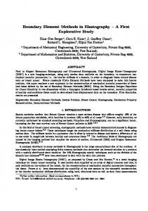
Figure 1. Numerical and exact evaluation of the convolution

U (t) H(t). 10

To check the procedure, the convolution between the fundamental solution of the displacep ment (r = ri ri with ri = xi yi )

Uij (x; y; t ) = ( 1 t 3rirj ij H t r H t r + 4% r2 r3 r c1 c2 " # ) rirj 1 t r 1 t r + ij t r (14) r3 c21 c1 c22 c2 c2 rc22 and the unit step function H (t) are calculated. Figure 1 shows the numerical and exact evaluation of the convolution integral U10 (t) H (t). Obviously, the agreement of the analytical and numerical solution is good, with the exception of the neighbourhood of the jumps. There, an overshooting is observed depending on the choice of the multistep method and the time step size t. The parameters in this test are chosen as suggested above with = 10 10. The used multistep method is a backward differential formula of second order. 3. BE Formulation For consistency, the boundary integral equation for elastodynamics in time domain is recalled. The field equations of a homogeneous elastic domain (Young’s Modulus E , density % and Poisson’s ratio ) are given by

c22 )ui;ij + c22 uj;ii + b%j = uj with displacements uj and wave speeds c21 = %(1 E (21 )(1 )+ ) ; c22 = %2(1E+ ) : (c21

(15)

(16)

In the above equations, ( );i denotes the derivative with respect to the spatial coordinate xi , and u j is the acceleration. On the boundary = u [ t of the domain , the boundary conditions

ti(x; t) = ij nj = pi(x; t) x 2 t;

ui(x; t) = qi(x; t) x 2

u

(17)

mec2042.tex; 26/08/1997; 12:27; v.7; p.4


183

are given. ij is the stress tensor and nj the outward normal on the boundary . For a complete initial boundary value problem also the initial conditions ui (x; 0) and u_ i (x; 0); x 2 , have to be prescribed. Here, they are assumed to be zero

ui(x; 0) = 0;

u_ i (x; 0) = 0

x 2 :

(18)

Assuming also vanishing volume forces, the dynamic extension of Betti’s reciprocal work theorem leads to the integral equation (see [2])

cij (y)uj (y; t) =

Z

x

[Uij (x; y; t) tj (x; t) Tij (x; y; t) uj (x; t)] d x ;

(19)

where Uij and Tij are the time-dependent fundamental solutions of the displacements and tractions, respectively. The integral free term cij (y) is the same as in elastostatics [14], e.g., cij (y) = ij =2 for a smooth boundary. As shown by Bonnet [3], the first integral in Equation (19) is weakly and the second strongly singular. Therefore, the second integral can only be defined in the sense of a Cauchy Principal Value. For the numerical solution of the boundary integral Equation (19) in an arbitrary domain , a discretization must be introduced. Therefore, the boundary is divided in E iso-parametric elements e where F polynomial shape functions Nef (x) for the spatial variable are defined. This procedure yields

E X E X F F X X ef f uj (x; t) = Ne (x)uj (t); tj (x; t) = Nef (x)tefj (t); e=1 f =1

(20)

e=1 f =1 ef with the time dependent nodal values uef j (t) and tj (t). Inserting these ‘ansatz’ functions in

Equation (19) leads to

cij (y)uj (y; t) =

E X F Z X e=1 f =1

I

e

e

Uij (x; y; t)Nef (x) d e tefj (t)

Tij (x; y; t)Nef (x)d e uefj (t)

:

(21)

If the time t is discretized in N equal time steps t, the convolution between the fundamental ef solutions Uij or Tij and the nodal values tef j (t) or uj (t), respectively, is approximated by the Convolution Quadrature formula (12). This results in the new boundary element formulation in time domain

cij (y)uj (y; nt) =

E X F X n X ^ y; t)tef f!nef k (U; j (kt)

e=1 f =1 k=0 ^ y; t)uef !nef k (T; j (kt)g

(22)

for n = 0; 1; : : : ; N , with the weights

^ y; t) = !nef (U;

r n LX1 Z U^ x; y; (r`) N f (x) d n; e ` e L `=0 e t

for the displacements (`

(23)

= ei` L ) and a similar expression for the weights of the tractions. 2

mec2042.tex; 26/08/1997; 12:27; v.7; p.5

184


Figure 2. Discretization, loading and boundary conditions of the bar.

Figure 3. Longitudinal displacement at point P versus time for different values of

t.

Note that the calculation of the integration weights (23) is only based on the Laplace transformed fundamental solution. Therefore, for the spatial integration in Equation (23), the techniques well known from the elastodynamic frequency domain formulation are used. Finally, Equation (22) is solved with the collocation method and a direct equation solver. 4. Numerical Example

N ; = 0; % = 1 kg ) As a first application, a bar (geometry: 3 m 1 m 1 m, material: E = 1 m 2 m3 is considered (see Figure 2). The bar is taken to be fixed on one end, and is loaded with a unit step function in time on the other free end. The remaining surfaces are traction free. The bar is discretized with 56 triangles, and linear shape functions p are used. The parameter r and L are chosen as suggested in Section 2: L = N and rN = , with the error bound = 10 10 . Smaller values of , e.g., below = 10 30 , lead to completely unstable results. The spatial integration is done with standard Gauß quadrature formulas. The weakly singular integrals in Equation (22) are regularized with a coordinate transformation and the strongly singular integrals with the method suggested by [5]. Results for the longitudinal displacement at the point P versus time are plotted for different time step sizes in Figure 3. There, a backward differential formula of second order is applied for the underlying multistep method. These results are compared with the 1-d solution [4], which is denoted with ‘exact’. Obviously, there exists a critical value of the time step size, below

mec2042.tex; 26/08/1997; 12:27; v.7; p.6


185

Figure 4. Comparison of different multistep methods.

which the results are unstable (t < 0:15). This is in accordance with the investigations for the boundary integral equation of the wave equation by [9]. For larger time step sizes (t = 0:9), a kind of phase shifting is observed because the time step size is too large to approximate the peaks correctly. Since the method suggested by Antes [2] shows an unstable behaviour using small time steps and numerical damping for large time steps, the time step size has there be restricted to the interval [0.7, 1.0]. In comparison with this formulation, here, a smaller lower critical value and no numerical damping is observed. However, this behaviour depends heavily on the underlying multistep method. Therefore, finally the influence of the underlying multistep method is studied in Figure 4. There, the results with a backward differentiation formula of the first order (BDF 1) and those of the second order (BDF 2) are compared. An optimal choice of the time step size t is used in both calculations. The results of the BDF 2 are closer to the 1-d solution than the results of BDF 1, but with the BDF 1 procedure much smaller time step sizes are possible.

5. Conclusions The present paper describes a boundary element formulation directly in time domain where only the fundamental solutions in Laplace domain are used. This formulation is based on the ‘Operational Quadrature Methods’ developed by Lubich [7]. Applying these quadrature formulas to the convolution integral in the boundary integral equation, a numerical integration formula is obtained where the weights depend only on the Laplace transformed fundamental solutions. With these formulas, a new time domain boundary element formulation is derived. A numerical example shows that a critical time step size exists, below which the method becomes unstable. This critical value depends on the underlying multistep method. Compared with the direct time domain based formulation suggested by [2], the critical time step size is much smaller. Furthermore, all advantages of the Laplace domain boundary element formulation can be used. Therefore, this method seems to be suitable also in the case of the hypersingular traction boundary integral equation, and for all cases where the time-dependent fundamental solution is not known, e.g., in viscoelasticity or poroelasto dynamics.

mec2042.tex; 26/08/1997; 12:27; v.7; p.7

186


References 1. 2. 3. 4. 5. 6. 7. 8. 9. 10. 11. 12. 13. 14. 15.

Ahmad, S. and Manolis, G.D., ‘Dynamic analysis of 3-d structures by a transformed boundary element method’, Computational Mechanics, 2 (1987) 185–196. Antes, H., Anwendungen der Methode der Randelemente in der Elastodynamik und der Fluiddynamik, Mathematische Methoden in der Technik 9, B. G. Teubner, Stuttgart, 1988. Bonnet, M., ‘Regular boundary integral equations for three-dimensional finite or infinite bodies with and without curved cracks in elastodynamics’, in Brebbia, C.A., Zamani, N.G., (Eds.), Boundary Element Techniques: Applications in Engineering, Southampton, Computational Mechanics Publications, 1989. Graff, K. F., Wave Motion in Elastic Solids, Oxford University Press, 1975. Guiggiani, M. and Gigante, A., ‘A general algorithm for multidimensional cauchy principal value integrals in the boundary element method’, ASME Journal of Applied Mechanics, 57 (1990) 906–915. Jäger, M., Entwicklung eines effizienten Randelementverfahrens für bewegte Schallquellen, Braunschweiger Schriften zur Mechanik 17-1994, Technische Universität Braunschweig, 1994. Lubich, C., ‘Convolution quadrature and discretized operational calculus. I.’, Numerische Mathematik, 52 (1988) 129–145. Lubich, C., ‘Convolution quadrature and discretized operational calculus. II.’, Numerische Mathematik, 52 (1988) 413–425. Lubich, Ch., ‘On the multistep time dicretization of linear initial-boundary value problems and their boundary integral equations’, Numerische Mathematik, 67 (1994) 365–389. Lubich, Ch. and Schneider, R., ‘Time discretization of parabolic boundary integral equations’, Numerische Mathematik, 63 (1992) 455–481. Mansur, W. J., A Time-Stepping technique to solve wave propagation problems using the boundary Element Method, PhD thesis, University of Southampton, 1983. Schanz, M., Eine Randelementformulierung im Zeitbereich mit verallgemeinerten viskoelastischen Stoffgesetzen, Bericht aus dem Institut A für Mechanik Heft 1, Universität Stuttgart, 1994. Schanz, M., Gaul, L. and Antes, H., ‘Numerical damping and instability of a 3-d BEM time-stepping algorithm’, Extended Abstracts of IABEM 93, Braunschweig, 1993. Steinfeld, B., Numerische Berechnung dreidimensionaler Kontaktprobleme Bauwerk-Boden mittels zeitabhängiger Randintegralgleichungen der Elastodynamik, Technisch wissenschaftliche Mitteilungen Nr. 93-1, Ruhr-Universität Bochum, 1993. Wiebe, Th. and Antes, H., ‘A time domain integral formulation of dynamic poroelasticity’, Acta Mechanica, 90 (1991) 125–137.

mec2042.tex; 26/08/1997; 12:27; v.7; p.8