InfoMod: A visual and computational approach to Gauss' binary ...

arXiv:1704.00902v1 [math.NT] 4 Apr 2017

InfoMod: A visual and computational approach to Gauss’ binary quadratic forms Ayberk Zeytin∗, Hakan Ayral∗, A. Muhammed Uluda˘g∗ April 5, 2017 Abstract InfoMod is a new software and application devoted to the modular group, PSL2 (Z). It has algorithms that deals with the classical correspondences among continued fractions, geodesics on the modular surface and binary quadratic forms. In addition the software implements the recently discovered representation of Gauss’ indefinite binary quadratic forms and their classes in terms of certain infinite planar graphs (dessins) called c¸arks. InfoMod illustrates various aspects of these forms, i.e. Gauss’ reduction algorithm, the representation problem of forms, ambiguous and reciprocal forms. It can be used as an educational tool, and might be used to explore some new facts about these objects.

1

Introduction

InfoMod is an innovative software which aims to visualize the deep arithmetic questions encircled by finitely generated infinite index subgroups of the modular group, which is by definition the the group consisting of 2 × 2 integral matrices of determinant 1, denoted by PSL2 (Z). These lead to the study of algebraic number theory of real quadratic number fields. Its intended use is instructive as well as research-level visual explorations of the modular group, binary quadratic forms, their geodesics, form classes, class groups and some algorithms such as Gauss’ reduction algorithm. One of the main problems of algebraic number theory is to understand factorization in the ring of integers of number field. The class group and its size, called the class number, are the prime indicators of how unique factorization in a ring of integer is. There are several important questions and conjectures about class groups and class numbers. One needs to recourse to algorithms for explicit computations of these groups. Since these problems resisted centuries of attacks, these are also important from the computational perspective and present many challenges. 1 Galatasaray

University, C ¸ iragan Cad. No 36 Be¸siktas¸s 34349 Istanbul, Turkey ¨ ITAK ˙ This work is supported by the TUB grant 113R017 and the GSU grant 15.504.002.

1

The simplest case of quadratic number fields, can be understood in terms of the binary quadratic forms of Gauss. Here the main difficulty is in the real quadratic case, which corresponds to indefinite binary quadratic forms. These forms can be represented as the fixed points of the elements of the modular group, and this group is the main hero of our paper. The modular group is isomorphic to the free product Z/2Z ∗ Z/3Z. As such its elements can be represented as the set of half-edges of an infinite rooted bipartite tree FT with a planar structure, called the Farey tree. In order to visualize the elements of FT , we broaden the branches of FT until they touch each other. The resulting mantra-like model of PSL2 (Z) with cells representing its elements, fills the entire plane and is called the sunburst. It allows one to simultaneously represent up to approx. 1000 elements of the modular group on a computer screen with a standard resolution. By moving the centre of this sunburst (operation which is implemented in InfoMod), it is possible to represent another 1000-element portion of the modular group. By clicking over a cell, it is possible to obtain a detailed information on the group element represented by this cell. In particular, it is possible to see the corresponding binary quadratic form as well as its discriminant. Now we alter our perspective slightly to get another representation of forms. Suppose that the element M ∈ PSL2 (Z) represents a reduced real binary quadratic form fM . As a matter of fact, every element different from identity in the subgroup hM i also represents the same reduced form. The group hM i acts on the tree F in a natural way, and the quotient graph FT /hM i also represents fM . Given an edge of the quotient graph, it is possible to recover the form. These graphs are called ¸carks. They look same as FT except that they have exactly one circuit inside, called the spine. InfoMod makes it possible to pass, from the cell of M , to its ¸cark. Many notions related to forms acquires a new formulation in terms of these graphs. For example, equivalent forms have isomorphic ¸carks. The reduction algorithm of Gauss simply moves the edge characterizing the form towards the spine of the ¸cark. This new formulation already served the first named author to give a solution of the representation problem of forms and improve on the Gauss reduction algorithm, [20]. InfoMod makes it possible to observe how these algorithms are carried out on the graph. Paper is organized as follows: In the next section we overview the theoretical background outlined in the above lines. More details can be found in [18]. The third section is devoted to the software implementation of InfoMod, where we present a code library which help represent and do computations on binary quadratic forms, including reductions and enumeration of other forms which share a cycle with a reduced form. Later we present an interactive visualization application to explore the mentioned sunburst and ¸carks visually. We plan to build into InfoMod some new features pertaining to the outer automorphism of the group PGL(2, Z) in the future.

2

2

Preliminaries

This section is devoted to recalling the basic facts around the modular group, binary quadratic forms, reduction theory and c¸arks. There are many beautiful texts on the subject among which we must note the first historically systematic treatment by Gauss, [8]. We refer to [2, 3] for a modern treatment of the topics related to binary quadratic forms.

2.1

Modular group, binary quadratic forms and geodesics

The modular group, PSL2 (Z), acts on the upperhalf plane  H = {z ∈ C : Im(z) > p q 0} via M¨ obius transformations, i.e. for W = ∈ PSL2 (Z) and z ∈ H, r s pz+q we have W · z := rz+s . This action leaves the Poincar´e metric on H invariant. Hence the geodesics of this metric, i.e. lines that are vertical to the real line and half circles whose centers are on the real line, are mapped onto geodesics by PSL2 (Z). An integral binary quadratic form (or BQF for short) is a homogeneous polynomial of degree two in two variables with integer coefficients. A BQF f(x, y) =  ax2 + bxy + cy 2 , is usually denoted by (a, b, c) or its matrix form a b/2 . We call f primitive if the greatest common divisor of a, b and c b/2 c is 1.   p q An element W = ∈ PSL2 (Z) has two fixed points, which are, by r s definition, roots of the quadratic equation rz 2 + (s
− p)z − q = 0. To W we associate the BQF fW := 1δ rx2 + (s − p)xy − qy 2 ; where δ is the greatest common divisor of r, s − p and q, so that fW is by definition primitive. The discriminant of a BQF f = (a, b, c) is defined as ∆(f ) = b2 − 4ac. A BQF is called degenerate if ∆(f ) is a perfect square, positive definite if ∆(f ) < 0 and a > 0, negative definite if ∆(f ) < 0 and a < 0. Finally, a BQF is called indefinite if ∆(f ) > 0. We may classify elements on PSL2 (Z) according to their traces. Namely, W is called elliptic, parabolic and hyperbolic if |Tr(W )| < 2, |Tr(W )| = 2 and |Tr(W ) > 2, respectively. In other words, parabolic elements have a unique real fixed point. Elliptic elements have two fixed points one in the upper half plane and the other in the lower half plane. Hyperbolic elements have two distinct real fixed points. The geodesic in H joining the two fixed points of a hyperbolic element W p ∈ PSL2 (Z)1 which is merely a half circle of center 1 (p − s)/2r and radius 2r Tr(W )2 − 4 is called the geodesic associated to W and denoted by γW . Observe that the classification of elements of PSL2 (Z) and BQFs are quite parallel. Namely, parabolic elements give rise to degenerate BQFs, elliptic elements give rise to definite BQFs and hyperbolic elements give rise to indefinite BQFs. 1 One may define attracting and repelling fixed points of W by looking at its action along this geodesic. This distinction is unnecessary for our purposes.

3

2.2

Reduction Theory of BQFs

The modular group acts on the set F of non-degenerate binary quadratic forms by  change  of variables. More precisely, given f = (a, b, c) and an element Mo = p q we define Mo · f to be the BQF associated to the symmetric matrix r s Mot Mf Mo ; where Mot stands for the transpose of Mo . In particular, we say that two forms f = (a, b, c) and f 0 = (a0 , b0 , c0 ) are equivalent if there is an Mo ∈ PSL2 (Z) so that Mo · f = f 0 . This action leaves the discriminant ∆ invariant, that is ∆(f ) = ∆(f 0 ) if f and f 0 are equivalent, and the equivalence class of a form f is denoted by [f ]. Therefore PSL2 (Z) acts on the set of nondegenerate BQFs of the same discriminant, say a square-free integer ∆, denoted by F(∆). In the search for a canonical representative of each p class, in [8], Gauss have defined a form f = (a, b, c) to be reduced whenever ∆(f ) − 2 |a| < b < p ∆(f ). It turns out that whenever f is definite (positive of negative) then there is a unique reduced BQF in its class, [f ]. If f is indefinite, then there are at least two reduced forms in [f ]. Gauss have also given an algorithm which takes any non-degenerate BQF as an input and produces an equivalent reduced BQF, described in [8]. One must note that there are other inequivalent notions of being reduced. For instance, Lagrange defines a BQF, say f = (a, b, c), to be reduced when |b| ≤ a ≤ c and b ≥ 0 if either a = c or |b| = a. Just as in the case of Gauss, every PSL2 (Z)-class of a positive definite BQF contains a unique Lagrange reduced form which can be found by the an algorithm that takes any non-degenerate BQF as input and produces an equivalent Lagrange reduced BQF, see the proof of [5, Theorem 2.8]. According to Zagier, p p p an indefinite p BQF is called reduced if both ∆(f ) < b < ∆(f ) + 2a and ∆(f ) < b < ∆(f ) + 2c are satisfied by f = (a, b, c). We refer to [19, § 13] for further details.

2.3

Ideal classes in quadratic number fields

A field K is called a number field whenever it is a finite extension of Q. The dimension of K as a vector space over Q is called the degree of the extension and denoted by [K : Q]. K is called quadratic quadratic whenever [K : Q] = 2. In this case, √ one can always find a square-free integer d with the property that K = Q( d). If d > 0, then we say that the extension is real and if d < 0 then the extension The map · : K −→ K sending an element √ is called imaginary. √ α = a + b d to α := a − b d is the only non-trivial automorphism of K which, together with identity, √ form the Galois group of K. An element α ∈ Q( d) is called an algebraic integer if it is a root of a monic polynomial pα (x) ∈ Z[x]. It is not so hard to see that the set of algebraic integers √ in Q( d), which will be denoted by Od , depends on the square-free integer d in √ 1+ d the following manner: if d is congruent to 1 modulo 4 then Od = Z+ 2 Z, and √ Od = Z + dZ otherwise. In particular, Od is a Dedekind ring. The property of Od being a unique factorization domain (UFD) is equivalent to Od being

4

a principal ideal domain(PID). And for any given ideal, a, of Od there are at most 2 elements α and β of Od so that the ideal generated by α and β, denoted hα, βi, is equal to a. This means fractional ideals of K, that is two dimensional Z-modules, a, of K for which there is an element ka ∈ Z so that ka · a is an ideal of Od , can also be generated by at most 2 elements. Given a fractional √ ideal a = hα, βi, we say that the pair (α, β) is oriented if (αβ − βα)/ d > 0. The set of oriented fractional ideals is an abelian group under multiplication, denoted by I + (K). The subset of principal fractional ideals, that is subsets of the forms αOd ⊂ K where α ∈ K, is a subgroup of I + (K) denoted by P (K), and the quotient H + (K) = I + (K)/P (K) is called the narrow ideal class group of K. The ideal class group of K, denoted H(K), is defined as the quotient I(K)/P (K); where I(K) is the multiplicative group of fractional ideals of K. The group H(K) is naturally a subgroup of H + (K). H(K) is of index 2 if Od admits an element of norm −1 and H(K) and H + (K) are isomorphic if there are no elements of norm −1 in Od .

2.4

C ¸ arks and ideal classes

√ The orbit√of the geodesic γ in the upper half plane joining −1, marked with ◦, to e2π −1/3 , marked with •, is a bipartite ribbon graph2 √ in H, where the vertices decompose naturally into two sets V = {orbits of −1} and V• = ◦ √ {orbits of e2π −1/3 }. The orientation is induced from the orientation of H. This graph is called the (bipartite) Farey tree and denoted by FT , see Figure 1. Vertices of type ◦ are always of valency (or order or degree) 2 and vertices of type • are always of valency 3.

Figure 1: The Farey tree. Given any element W ∈ PSL2 (Z), by restricting the action of PSL2 (Z) on H to an action on FT we can consider the quotient of FT by the subgroup generated by W . The quotient is a bipartite ribbon graph which we refer to as a ¸cark. The classification of elements of PSL2 (Z) reflects itself in its ¸cark, see Figure 2. 2 A bipartite graph is a graph whose vertices can be decomposed into two disjoint sets so that no two edge belonging to the same set are joined by an edge. A ribbon graph is a graph together with a cyclic ordering of edges emanating from each vertex.

5

Figure 2: Elliptic, parabolic and hyperbolic ¸carks, respectively. When W is elliptic of order 2 or 3 we obtain a rooted tree. If W is parabolic then the corresponding ¸cark has a unique cycle, named spine, which is assumed to be oriented counter-clock-wise and finitely many rooted trees attached to this cycle each of which is a rooted tree attached to vertices of type • of the spine. Such components are called Farey components of the c¸ark. They all point outwards. When W is hyperbolic, once again the graph has a unique cycle, named spine, having finitely many vertices. To each vertex of type • there is a Farey component attached. In this case, Farey components must point both inwards and outwards. As a result of the construction the cosets γ ·hW i ∈ PSL2 (Z)/hW i correspond in a one to one fashion to edges of the ¸cark FT /hW i. So we conclude that there is a one to one correspondence between the set of edges of the ¸cark corresponding to the form fW and element of the equivalence class [f ], see [18, § 2] for details.

3 3.1

Software Design Components

InfoMod consists of a shared library coded in C for computationaly heavy functions, some convenience wrapper classes for Matlab and Python to facilitate interfacing the library, and a visualization application written in ActionScript version 3. The native code shared library implements the computation of the two methods of reduction (¸cark and Gauss), enumeration of quadratic forms residing on a spine and computation of the signature of a spine. On the other hand wrap-

6

per classes to access the library from Matlab and Python environments provide an easy way to invoke library functions, while providing an Object Oriented representation for the involved quadratic forms. Source code for Matlab and Python libraries are available online https://github.com/hayral/infomod. Many functions which aren’t computationaly demanding, such as evaluating a form at a point, obtaining the matrix representation of the form, or querying the spinality, primitivity and reducedness, are implemented in the wrapper classes, as the overhead of function invocation from dynamic library outweights the benefits for those cases.

Figure 3: BinaryQuadraticForm class in Matlab and Python wrapping lowlevel reduction library and providing some convenience functions. (parameter and return types seen on figure are for UML diagramming purposes, actual implementation types differ according to Matlab/Python environment )

3.2

Visualization of the modular group and Sunburst

While Matlab and Python libraries are designed to be used as part of other computational code, the interactive visualization application of InfoMod is designed as an exploration tool to provide insight. It uses the same code base as the libraries, but ported to ActionScript programming language; as we planned to deploy this application to web and mobile, invoking our native code shared library or relying on Matlab/Python was not an option. Before elaborating on the visualization aspect of the software, let us define the underlying mathematical structure that visualization is designed to explore.   0 −1 Modular group is generated by two torsion elements S = and 1 0

7



 1 −1 of orders 2 and 3, respectively. There are no relations among 1 0 S and L hence we have the isomorphism PSL2 (Z) ∼ = Z/2Z ∗ Z/3Z. So every element in PSL2 (Z) can be written as a word in S, L and L2 . Without loss of generality, we assume that the length of words, denoted by `(W ), are of minimal length3 . Given two words W and W 0 in PSL2 (Z), by W ∩ W 0 we denote the word which is equal to the common initial part of the words W and W 0 . For instance, for W = (LS)2 (L2 S)3 LSL and W 0 = (LS)2 (L2 S)3 L2 SLSL2 we have W ∩ W 0 = (LS)2 (L2 S)3 . Let us now construct the slit disk, which we denote by D. We start with a standard disk, split into three equal area pieces by lines from the center of the disk. The so obtained three cells are labeled as I, L and L2 . To the circumference of this disk we glue an annulus which is also divided in 3 pieces by prolonging the lines that were used to divide the initial disk. This time, the 3 new cells are identified with S, LS and L2 S, respectively. The next step is to attach two annuli each of which is divided evenly into 6 pieces via first prolonging the existing lines and then adding 3 more lines so that the cell labeled S is neighbors with the cells SL and SL2 , and these are in turn neighbors with SLS and SL2 S in the second annulus. Similarly, the cell labeled LS is neighbors with the cells LSL and LSL2 , and these are in turn neighbors with LSLS and LSL2 S in the second annulus and finally the cell labeled L2 S is neighbors with the cells L2 SL and L2 SL2 , and these are in turn neighbors with L2 SLS and L2 SL2 S in the second annulus. Inductively, we obtain a disk, to which we will refer as the slit disk, where each cell is labeled with a word in S, L and L2 see Figure 4. As a result of the construction given above we have a one to one correspondence between elements of PSL2 (Z) and cells in D. If the a cell in D is labeled as W and ending with L or L2 then there are 4 cells surrounding it: three of them are labeled with W L, W L2 and W S. Remark that `(W ∩ W 0 ) ≥ `(W ) − 1 where W 0 is one of W L, W L2 or W L2 . The fourth neighbor, say W 00 , of W satisfies `(W ∩ W 00 ) ≤ `(W ) − 2 with `(W ) = `(W 00 ). Similarly, if W is a word ending with S, then there are 5 cells surrounding this cell. Three of them, which satisfies `(W ∩ W 0 ) ≥ `(W ) − 1, are labeled with W L, W L2 and W S. The remaining two words W 00 and W 000 satisfy `(W ) = `(W 00 ) = `(W 000 ) and `(W ∩W 00 ) < `(W )−2 and `(W ∩W 000 ) < `(W )−2. L=

3 The length of a word is defined to be the number of letters (L, L2 and S) appearing in the word.

8

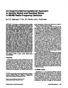
Figure 4: Main display of InfoMod The main visualization of the application is the above described slit disc (sunburst) type diagram. When the user moves the mouse pointer over one of the cells on D, a blue line indicates the path to the center of the disc as it passes by the centers of the parent cells. Due to the exponential growth of the number of child nodes on a binary tree, this sunburst type visualization can only depict eight levels of depth for common mobile device and desktop screen resolutions. Once a cell representing an element of PSL2 (Z) is left clicked, a radial menu appears with options. Apart from the elements in the menu related to the visualization of the corresponding binary quadratic form along with its neighbors the button “Move to Center” is used to interact with elements of the modular group which are at depth nine or further. Namely, on click by conjugation, the chosen element becomes the center of the displayed D and all the other elements are translated accordingly. In this fashion, one may travel arbitrarily far from the actual center.

9

Figure 5: Radial menu on web application and main screen on mobile application Challenges implementing the web and mobile visualization app ActionScript isn’t designed with scientific computing or high performance computing as primary concern, but it has all the features of a modern managed object oriented language [6], and provides access to hardware accelerated graphics capabilities of the underlying operating system. Flash runtime is generally deployed in the form of a browser plugin (Flash Player), but standalone applications can be deployed as independent executables without requiring being embedded in a browser. ActionScript and the Flash Runtime has no direct access to mathematical computing libraries; therefore one of the challenges was the necessity to implement all mathematical structures and computation codes from scratch; including a class to represent a binary quadratic form, a class to represent an element from the modular group, and minimal linear algebra to operate on the matrix representation of elements of modular group4 . Another challenge was the code being run by a JIT compiling VM with automatic garbage collection which is the Flash Runtime. Even though we didn’t need C/C++ like native code speed, having numerous visual objects (up to the order of 212 ) visible on the screen with many destroyed and some newly created at each user interaction cause a heavy burden on the garbage collector; therefore we employed some object pooling and caching methods to maintain interactive speeds and minimize stutter caused by garbage collector. Another challenge was to port the same application to mobile platforms, namely Android and iOS. AIR compiler provides platform independence to some degree, but user experience is not the same due to differences on hardware features. One of the 4 Standard ActionScript libraries do provide a native 3 × 3 matrix class, but in our case we needed some extra functions like trace,transpose and multiplication with specific constants (i.e. generators of modular group and some of their compositions) which reduces to simple swap and sign change of values when optimized.

10

two main manifestations of this are the resolution and aspect ratio differences of different mobile devices requiring the size and placement of visual objects to be flexible and independent of screen size (including fonts and text rendering which is not as fast and flexible on mobile platforms); and the other being the relatively limited resources in terms of computing power and memory.

3.3

Visualization of the ¸carks and geodesics

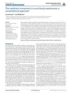
Let us now fix a hyperbolic element W ∈ PSL2 (Z). The c¸ark visualization consists of edges forming the spine (which are called semi-reduced ) and the rooted Farey trees attached to it. The correspondence between edges of FT /hW i and forms f that are equivalent to fW can be investigated by hovering the mouse cursor over, thus highlighting the edge green and updating the top left corner green label with the corresponding forms expression. The form corresponding to W is indicated as a red edge, and has a label for its expression on top left.

Figure 6: Visualizations of c¸ark for form (-14,2,1). (left) As rendered by visualization application, and some branches expanded through interaction (right) As rendered by plot cark() method of Matlab wrapper class Every non-reduced form in the equivalence class (i.e. edges not on the spine) can be clicked on to expand the child edges, and the whole graph re-scales and positions itself to fit on available screen space; yet as the trees are infinite deeper child edges get smaller angular ranges to position themselves. Every quadratic form on the spine of the ¸cark also corresponds to a geodesic in upper half-plane. Once an edge is selected on the c¸ark visualization, the geodesic of the form corresponding to selected edge can be plotted, both in H or in the unit disk, D = {z ∈ C : |z| < 1}.

11

Figure 7: Visualization of the geodesics (left) Upper half plane model (right) Disc model Flips There is a close relationship between mapping class groups of surfaces of genus g with n punctures and the groupoid whose objects are bipartite ribbon graphs of genus g with n punctures and morphisms are flips (or Whitehead moves or HI moves), see Figure 8. Indeed, flips do not change the invariants g and n and act transitively on the set of ribbon graphs of fixed g and n. Then, as a result of a generalization of Dehn-Nielsen-Baer theorem, [7, Theorem 4.8], we obtain the required injection. InfoMod can make explicit computations using flips in the case of annulus.

Figure 8: (left) Flip action on ribbon graphs (right) Visualization of intervals exchanged on the boundary of the disk for a specific flip

4

Representation problem

Representation problem deals with the existence and values of integer solutions, that makes a given binary quadratic form equal to a chosen integer. For the positive definite forms if integer solutions exist, they are finitely many; on the other hand for indefinite case if an integer solution exists, then there is a family of countably infinite pairs of integers. Each solution pair (x, y) can be obtained by multiplying a non-trivial solution with an automorphism of the form of appropriate order. 12

It must be mentioned that there is a non-exact algorithm presented on the web-page “https://www.alpertron.com.ar/quad.java”. In addition, in [14] Lagrange has put forward a method to solve similar equations which run in exponential time, which are then further optimized in [15]. Some related algorithms have been investigated in [13]. Pell equation is another class of such equations whose theory is well developed, [10]. In [9] equations of the form aX 2 −bY 2 = N are discussed. Algorithms concerning the case N = −1 (sometimes referred to as non-Pellian equation), have been discussed by Lagarias in [12]. In [12] Lagarias proposes a modification to classical reduction method, through which he established a worst case time complexity of O(nµ(n)) with µ(n) being the time complexity of the chosen n-bit multiplication algorithm, yielding O(n3 ) in case regular multiplication is employed. In [1] Buchmann improves the complexity analysis of Lagarias to O(n2 ) without changing the algorithm, using the observation that if for a form f neither f, ρ(f ) or ρ2 (f ) 5 is reduced then the absolute value of the first coefficient (a) must be at least twice the absolute value of the last coefficient (c). Eventhough a faster reduction algorithm of O(log(n)µ(n)) time complexity is presented earlier by Schnhage [16], the asymptotic acceleration surpasses the other algorithms only when the number of binary digits of the coefficients of the form to be reduced is in the order of 104 or greater. The representation problem is closely related to class group computations in quadratic number fields. For instance, in [17], Shanks developed a new method for the computation of class numbers of quadratic number fields, which further resulted in a new factorization of large integers. The thesis of Jacobson, [11], discusses such algorithms in detail. Similar results for general number fields are presented in [4]. Here, we present an algorithm to solve the representation problem given a binary quadratic form and an integer to solve for. The algorithm relies on two things: first to find another form which is part of a face with label equal to given integer if such a face exists (or to show that such a face doesn’t exist), and second to compute the path leading from this form found to the form given. Equipped with reduction and graph topology of c¸arks, the computation of integer solutions proceeds as follows: First the software performs the reduction while recording the path down to the spine of its c¸ark as a sequence of PSL2 (Z) generators (algorithm 1,line 2), then it travels along the spine and this time it records the forms belonging to spine as a sequence (l.4). Depending on the sign of the chosen integer to solve the quadratic form for, software generates all non-spinal neighbours of recorded spinal forms, but records only those with coefficients having same sign as the chosen integer (l.8-17). This list of non-spinal neighbours of the same sign with desired integer, serves as the root nodes of a simultaneous breadth-first search along the graph of the spine (l. 18-36). This breadth-first search travels away from the spine (inwards or outwards depending on the sign). Even though every form yields two new forms once expanded 5 with

 ρ being the reduction operator, defined as f U (f ) and U (f ) =

13

0 1

 −1 s(f )

Algorithm 1 Solver for Representation Problem Require: fstart is form object, N is an integer 1: function SolveForm(fstart ,N ) 2: path1 ← CarkReducePath(fstart ) . path from fstart to spine 3: entryP oint1 ← path1 ( len(path1 ) ) . last form on path1 (it’s on spine) 4: spineF orms ← RevolveAroundSpine(entryP oint) . all forms on spine 5: f ormsT  oSearch  ← ∅  1 −1 0 −1 6: L← ,S ← . PSL2 (Z) generators 1 0 1 0 7: e1 ← (1, 0), e2 ← (0, 1) . e1 , e2 : standard oriented basis of Z2 8: for each f in spineF orms do . neighbours of spine 9: f1 ← f · L . PSL2 (Z) group action 10: f2 ← f · L2 11: if (f1 (e1 ) × f1 (e2 ) > 0) ∧ (f1 (e1 ) × N > 0) then 12: f ormsT oSearch = f ormsT oSearch ∪ {f1 } 13: end if 14: if (f2 (e1 ) × f2 (e2 ) > 0) ∧ (f2 (e1 ) × N > 0) then 15: f ormsT oSearch = f ormsT oSearch ∪ {f2 } 16: end if 17: end for 18: temp ← ∅ 19: while f ormsT oSearch 6= ∅ do . breadth-first search 20: for each f ∈ f ormsT oSearch do 21: if (f (e1 ) = N ) ∨ (f (e2 ) = N ) then 22: ff ound ← f . ff ound : first form on the face with label N 23: break . leave the while loop 24: else 25: f1 ← f · S · L . PSL2 (Z) group action 26: f2 ← f · S · L2 27: if (abs(f1 (e1 )) < abs(N )) ∧ (abs(f1 (e2 )) < abs(N )) then 28: temp = temp ∪ {f1 } 29: end if 30: if (abs(f2 (e1 )) < abs(N )) ∧ (abs(f2 (e2 )) < abs(N )) then 31: temp = temp ∪ {f2 } 32: end if 33: end if 34: end for 35: f ormsT oSearch ← temp, temp ← ∅ . swap the lists 36: end while 37: if targetF orm = ∅ then 38: return ∅ . no integer solution 39: else 40: path2 ← CarkReducePath(ff ound ) . path from ff ound to spine 41: entryP oint2 ← path2 ( len(path2 ) ) . last form on path2 (it’s on spine) 42: path3 ← PathOnSpine(entryP oint2 , entryP oint1 ) . path on spine between entry points 43: path4 ← path2 + path3 + ReversePath(path1 ) . path from ff ound to fstart 44: M ← PathToMatrix(path4 ) 45: if fstart (e1 · M ) = N then 46: return e1 · M 47: else 48: return e2 · M 49: end if 50: end if 51: end function

14

on the direction of increasing distance, the number of accumulated forms does not increase exponentially; the reason for this boils down to the coefficients of neighbouring forms growing or decreasing (depending on the travel being directed towards or away from the spine) at a non-linear speed when multiple forms are traversed. At each iteration of breadth-first search software compares the absolute value of the coefficients of the newly expanded forms with the absolute value of the integer being searched, and discards the form if the first or last coefficient of the form is greater than this in absolute value (l.27-32). If all the forms on breadth-fist search list gets discarded, the loop terminates (l.19) and algorithm doesn’t return an integer pair, indicating that there are no integer solutions (l.37-38). If the search finds a form adjacent to a face with chosen label, it breaks from the loop after marking the found form (l.21-23), and the path from the found form and its entry point to spine is calculated (l.40-41). At this point as we have paths from both starting and found form to the spine; to build a continuous path from found form to starting form, we only need the path that connects the entry points of those paths to the spine. Once the complete paths missing part on the spine is calculated (l.42), they can be combined to build the path leading from found form to starting form (l.43). The rest is nothing more than converting this path which actually is a sequnce of generators on PSL2 (Z) to a matrix (l.44), and then to decide which of the two orthogonal basis solves the form when multiplied with the path in matrix form (l.45-49). For the algorithm listing of functions referenced in Algorithm.1 see Appendix, for the listing of ¸cark reduction algorithm see [20].

5

Conclusions

In this paper we present the software package InfoMod for representing and operating on binary quadratic forms. It consists of a library identically implemented in Matlab and Python6 , which can compute reduction of binary quadratic forms and solve the representation problem. It also contains an interactive visualization application available for web 7 and mobile 8 platforms, which allows to observe the intricate patterns of forms’ properties plotted according to their natural topology, and practically compute the reductions/representation problem solutions without writing code to invoke the libraries.

References [1] Ingrid Biehl and Johannes Buchmann. An analysis of the reduction algorithms for binary quadratic forms. In Voronoi’s Impact on Modern Science, pages 71–98, 1997. 6 source 7 8

code available at https://github.com/hayral/infomod http://math.gsu.edu.tr/azeytin/infomod/node/3 https://play.google.com/store/apps/details?id=air.com.hkn.infomod

15

[2] Johannes Buchmann and Ulrich Vollmer. Binary quadratic forms:An algorithmic approach, volume 20 of Algorithms and Computation in Mathematics. Springer, Berlin, 2007. [3] Duncan A. Buell. Binary quadratic forms. Classical theory and modern computations. New York, NY etc.: Springer-Verlag, 1989. [4] Henri Cohen, Francisco Diaz y Diaz, and Michel Olivier. Subexponential algorithms for class group and unit computations. J. Symb. Comput., 24(34):433–441, 1997. [5] David A. Cox. Primes of the form x2 +ny 2 . Pure and Applied Mathematics (Hoboken). John Wiley & Sons, Inc., Hoboken, NJ, second edition, 2013. Fermat, class field theory, and complex multiplication. [6] Stewart Crawford and Elizabeth Boese. Actionscript: a gentle introduction to programming. Journal of Computing Sciences in Colleges, 21(3):156– 168, 2006. [7] Benson Farb and Dan Margalit. A primer on mapping class groups. Princeton, NJ: Princeton University Press, 2011. [8] Carl Friedrich Gauss. Disquisitiones arithmeticae, volume 157. Yale University Press, 1966. [9] M. J. Jacobson, Jr. and H. C. Williams. Modular arithmetic on elements of small norm in quadratic fields. Des. Codes Cryptogr., 27(1-2):93–110, 2002. Special issue in honour of Ronald C. Mullin, Part II. [10] Michael J. Jacobson, Jr. and Hugh C. Williams. Solving the Pell equation. CMS Books in Mathematics/Ouvrages de Math´ematiques de la SMC. Springer, New York, 2009. [11] M.J. Jacobson Jr. Subexponential Class Group Computation in Quadratic Orders. PhD thesis, Technische Universit¨at Darmstadt, 1999. [12] J.C. Lagarias. On the computational complexity of determining the solvability or unsolvability of the equation X 2 − DY 2 = −1. Trans. Am. Math. Soc., 260:485–508, 1980. [13] J.C. Lagarias. Worst-case complexity bounds for algorithms in the theory of integral quadratic forms. J. Algorithms, 1:142–186, 1980. ¨ [14] J. L. Lagrange. Uber die L¨osung der unbestimmten Probleme zweiten Grades (1768). Aus dem Franz¨osischen u ¨bersetzt und herausgegeben von E. Netto. Leipzig: Wilhelm Engelmann. 131 S. 8◦ (Ostwalds Klassiker Nr. 146) (1904)., 1904.

16

[15] R.E. Sawilla, A.K. Silvester, and H.C. Williams. A new look at an old equation. In Algorithmic number theory. 8th international symposium, ANTSVIII Banff, Canada, May 17–22, 2008 Proceedings, pages 37–59. Berlin: Springer, 2008. [16] Arnold Sch¨ onhage. Fast reduction and composition of binary quadratic forms. In Proceedings of the 1991 international symposium on Symbolic and algebraic computation, pages 128–133. ACM, 1991. [17] Daniel Shanks. Class number, a theory of factorization, and genera. 1969 Number Theory Institute, Proc. Sympos. Pure Math. 20, 415-440 (1971)., 1971. [18] A. M. Uluda˘ g, A. Zeytin, and M. Durmu¸s. Binary quadratic forms as dessins. 2016. to appear in J. Th´eor. Nombres Bordeaux. [19] Don B. Zagier. Zetafunktionen und quadratische K¨ orper. Eine Einf¨ uhrung in die h¨ ohere Zahlentheorie. , 1981. [20] A. Zeytin. On reduction theory of binary quadratic forms. Publ. Math. Debrecen, 89:203–221, 2016.

APPENDIX In this section you can find the algorithm listings for the functions invoked by Algorithm 1: Representation Problem Solver. Algorithm 2 Generate All Spinal Forms Require: fspinal is a form on the spine 1: function RevolveAroundSpine(fspinal ) 2: e1 ←(1, 0), e2← (0, 1)  1 −1 0 −1 3: L← ,S ← 1 0 1 0 4: list ← ∅ 5: fnext ← fspinal 6: repeat 7: fnext ← fnext · SL 8: if fnext (e1 ) × fnext (e2 ) > 0 then 9: fnext ← fnext · L 10: end if 11: list ← list ∪ {fnext } 12: until fnext = fspinal 13: return list 14: end function

17

. e1 , e2 : standard oriented basis of Z2 . PSL2 (Z) generators

. PSL2 (Z) group action . multiply again to obtain L2

. repeat until we are back to starting form

Algorithm 3 Path Between Two Forms on Spine as a Word Require: ff rom and fto are forms on spine 1: function PathOnSpine(ff rom , fto ) 2: e1 ←(1, 0), e2← (0, 1)  1 −1 0 −1 3: L← ,S ← 1 0 1 0 4: path ← ε 5: fnext ← ff rom 6: repeat 7: fnext ← fnext · L 8: path ← path + ”L” 9: if fnext (e1 ) × fnext (e2 ) > 0 then 10: fnext ← fnext · L 11: path ← path + ”L” 12: end if 13: if fnext = fto then 14: break 15: end if 16: fnext ← fnext · S 17: path ← path + ”S” 18: until fnext = fto 19: return path 20: end function

. e1 , e2 : standard oriented basis of Z2 . PSL2 (Z) generators . empty string

. PSL2 (Z) group action . + : string concatenation . multiply again to obtain L2

. leave the loop early

. repeat until we arrive at fto

Algorithm 4 Convert a sequence of PSL2 (Z) generators represented as symbols from alphabet {S, L} to a 2 × 2 matrix Require: path is a sequence of symbols from alphabet {S, L} 1: functionPathToMatrix(path)      1 −1 0 −1 1 0 2: L← ,S ← ,M ← . L, S : PSL2 (Z) generators, M : 1 0 1 0 0 1 identity 3: for i ← 1.. Len(path) do 4: if path[i] = ”L” then 5: M ←M ·L 6: else 7: M ←M ·S 8: end if 9: end for 10: return M 11: end function

18