Investigating Parameters for Unsupervised Clustering of Speech

1

Investigating Parameters for Unsupervised Clustering of Speech Segments using TIMIT Lerato Lerato and Thomas Niesler Department of Electrical and Electronic Engineering University of Stellenbosch, South Africa {llerato, trn}@sun.ac.za

Abstract—We investigate the application of agglomerative clustering to short segments of speech signals. The successful direct clustering of such sub-word speech segments has direct application in the automatic derivation of pronunciation variants for use in automatic speech recognition (ASR) systems. We consider several configurations of hierarchical agglomerative clustering in order to determine the best configuration for the speech clustering task. Similarity between segments is computed by dynamic time warping (DTW), within which the application of Euclidean and city-block distance measures were evaluated. The effect of path length normalisation of the DTW score is considered, and finally the application of three different betweencluster distance measures is compared. Experiments are carried out on a subset of the phone segments present in the TIMIT database. We find that the city-block distance in conjunction with a normalised DTW score and the Ward cluster linkage method lead to best results.

I. I NTRODUCTION The objective of this paper is to investigate the parameters that influence the unsupervised clustering of short segments of speech data. Clustering spans many fields of pattern recognition, such as image processing, speech processing and document recognition. We focus on a speech processing application in which short segments of audio taken from a corpus of connected speech must automatically be grouped into different clusters in an effort to group similar sounds. In order to allow controlled experimentation and the evaluation of clustering results, the segments we consider are phone units taken from the TIMIT speech corpus. The unsupervised clustering of sub-word speech sounds has several applications in speech processing. One of these is the automatic generation of pronunciations for use in an automatic speech recognition (ASR) system. This application was considered in [1], where the authors bootstrap a system using grapheme-based subword models. Later work in which this restriction was removed indicated that careful attention to the clustering of audio segments would be required [2]. In this paper, we address this issue. Other applications of the type of clustering that we consider include automatic keyword discovery [3] in which frequently recurring words or phrases are detected in untranscribed audio. Mareuil et al [4] and Imperl et al [5] clustered speech segments from multiple languages for applications in multilingual speech recognition and language identification respectively. Mak and Barnard [6] cluster speech segments using agglomerative hierarchical clustering (AHC) in an approach that is similar to ours. They however use Gaussian

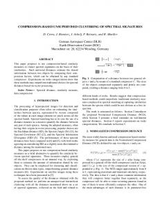
probability density functions and the Bhattacharyya distance to find the inter-cluster similarity. In contrast to the work covered in [2], we focus exclusively on the clustering problem and experiment with several configurations in order to determine how the parameters affect the performance of the algorithm. Neel [7] performs cluster analysis in various ways on TIMIT speech data. In this work however the number of clusters was fixed. We attempt unsupervised clustering in which the data are clustered purely on the basis of the feature representation. II. AGGLOMERATIVE HIERARCHICAL CLUSTERING Cluster analysis is the process of discovering the natural groupings of a set of patterns, points or objects [8], [9], [10], [11]. The analysis itself is based on the hypothesis that similarity between related points in the data set should be high while similarity between different points should be low. The points are then grouped according to this similarity. Agglomerative hierarchical clustering (AHC) is one approach to performing the grouping task. AHC is a bottom-up method that merges pairs of clusters according to a certain similarity measure. Initially each data point (speech segment) forms a singleton cluster. At this stage the number of clusters is equal to the number of speech segments. Subsequently clusters are merged in a pairwise fashion until a single cluster remains. This procedure generates a tree-like hierarchical grouping known as a dendrogram, as illustrated in Figure 1. In order to determine the similarity between two clusters, the similarity between individual members of the clusters must also be computed. These members are in our case segments of speech, and their similarity will be computed using dynamic time warping (DTW), which will be described in Section II-A. Furthermore, once the similarity between individual cluster members is known, the similarity between the clusters themselves can be computed in a variety of ways. Some of these linkage methods will be described in Section II-B. A. Dynamic time warping Dynamic time warping (DTW) is an algorithm that calculates the similarity between two sequences of generally unequal length. DTW was once the basis of template-based isolated-word speech recognition, but has been superseded by statistical techniques such as hidden Markov models (HMMs) [12], [13]. For our application, in which we would like

2.0

U and V are two clusters whose similarity must be measured. • K and L are the number of elements in U and V respectively. • When cluster U contains segment ci , we denote this by ci ∈ U . • d(ci , cj ) is the distance between two segments, as calculated by DTW. The average-link uses the average distance computed between all possible pairs of observations drawn from U and V . The criterion joins clusters with small variances and is less influenced by outliers than many other methods. It can mathematically be presented as: •

Inter−Cluster Similarity (Distance)

T3

T2

1.5

T1 0

ah

aa

ah

ix

ix

Cluster 1

iy

Cluster 2

w

uh

cluster 3

ah

ae

Cluster 4

Figure 1. An example of agglomerative hierarchical clustering (AHC) and the associated dendrogram.

to assess the similarity between two specific but otherwise arbitrary segments of speech, it is well-suited. Let the two speech segments in question be S1 (α) and S2 (ω), where α = 1, 2, . . ., A and ω = 1, 2, . . ., Ω. S1 = {X1 , X2 . . ., XA }, S2 = {Y1 , Y2 . . ., YΩ } and Xα or Yω are the T-dimensional feature vectors. Now consider a Ω×A local distance matrix, D, whose entries are the distances between all possible pairs of feature vectors from the two segments. The distance measures can be chosen to suit the application, and we will consider the Euclidean and the city-block distances in our evaluation. The Euclidean distance is given by: v u T uX d(Xα , Yω ) = t (xαi − yωi )2 (1) i=1

T X

|xαi − yωi |

X X 1 d(ci , cj ) K ×L

(3)

ci ∈U cj ∈V

The complete-link criterion considers the points in each cluster that are furthest apart. This can make it vulnerable to outliers as such anomalous points will often be the most distant. However it has the advantage of preferring compact clusters. It is calculated as: Simcomp (U, V ) =

max

ci ∈U,cj ∈V

d(ci , cj )

(4)

The Ward-link method considers the increase in the total intra-cluster sum-of-squares that results when two clusters are merged. This intra-cluster sum is defined as the sum of squares of the distances between all members of the cluster and its centroid. This method tends to join clusters with a small number of observations. It is mathematically presented as: 2

Simward =

kcU − cV k (1/K + 1/L)

(5)

2

while the city-block entry is expressed mathematically as: d(Xα , Yω ) =

Simave (U, V ) =

where kcU − cV k is the distance between the centroids, cU and cV , of clusters U and V respectively. (2)

i=1

From the matrix D, the best alignment between the sequences S1 (α) and S2 (ω) can be computed recursively by the principle of dynamic programming [13]. The score associated with this best alignment can then be taken as a measure of similarity between the two sequences. By dividing this score by the total length of the alignment path, a measure of the average per-frame similarity can be obtained. Both normalised and unnormalised versions of the DTW score will be considered in our experimental evaluation. B. Linkage methods Dynamic time warping allows the similarity between two individual speech segments to be evaluated. However, during clustering, the similarity between two clusters of segments must also be computed. There are several strategies to compute this inter-cluster similarity, and we have chosen three of these linkage methods for experimental evaluation: averagelink, complete-link and Ward-link [10], [11]. We will use the following notation for the description of the linkage methods:

III. C LUSTER EVALUATION In general, the clustering process will make errors, for example by placing two dissimilar segments in the same cluster, or by assigning similar segments to different clusters. Ideally, however, each cluster contains segments from only one phone, and all the segments of a particular phone belong to the same cluster. In order to to evaluate the success of the clustering process, we require measures that will indicate the extent to which these competing goals are achieved. Several methods have been proposed to accomplish this [14] and of these we have chosen two for our experimental evaluation. Let us consider our data to consist of N segments that belong to J different classes. Ideally1 the number of clusters K, also referred to as the cardinality, should equal the number of classes. Now assume the following notation: • G = {G1 , G2 , ..., GK } where G is the set of clusters and Gk is cluster k that contains speech segments. 1 This has the disadvantage of considering alternative groupings of acoustically similar clusters as errorful. We leave the analysis of this effect to future work, in which ASR evaluations are incorporated.

• •

C = {C1 , C2 , ..., CJ } where C is the set of classes and Cj is a set of phones with the same class. maxj |Gk ∩ Cj | represents the number of occurrences of the most frequent phone in cluster Gk .

A. Normalised mutual information The normalised mutual information (NMI) is based on the mutual information between classes and clusters [9],[14]. The mutual information is denoted by I(G, C) and is given by: I(G, C) =

X

X

P (Gk ∩ Cj ) log

Gk ∈G Cj ∈C

P (Gk ∩ Cj ) (6) P (Gk )P (Cj )

where P (Gk ), P (Cj ) and P (Gk ∩ Cj ) are the probabilities of a speech segment occurring in cluster Gk , in class Cj and in both cluster Gk and class Cj , respectively. The mutual information measure, I(G, C), does not penalise cardinalities. To make it sensitive to the varying number of clusters, it can be normalised by a factor based on the entropy of both clusters and classes. This normalising factor is given by: 1/2[H(G)+H(C)], where H(.) denotes the entropy. H(G) measures cluster cohesiveness [15] and is given by: X H(G) = − P (Gk ) log P (Gk ) (7)

Recall is given by: Rec =

TP TP + FN

(10)


where F N + T N = N2 − (T P + F P ),
PJ F N = i V2i − T P , Vi = |Ci ∩ Gj | and |Ci ∩ Gj | is the number of segments of one category in cluster j. The recall expression is the ratio of segments from the same class in the particular cluster to the total number of all segments that belong to the same class in all clusters. The F-measure is quantified as: F =

2 × P rc × Rec P rc + Rec

(11)

which can be further refined by introducing a mechanism that allows more weight to be assigned to recall or to precision. Let β be a constant and rewrite the F-measure as: Fβ =

(β 2 + 1) × P rc × Rec β 2 × P rc + Rec

(12)

We select β > 1 to give more weight to recall . When β = 1 Equation 12 simplifies to Equation 11.

Gk ∈G

H(C) is a measure of class cohesiveness and is calculated similarly. Normalising I(G, C) in this way makes it respond to cardinality, because entropy tends to increase with the number of clusters. The normalised mutual information criterion is therefore given by: I(G, C) (8) N M I(G, C) = 1 /2[H(G) + H(C)] The NMI is always a number between 0 and 1 where 1 denotes purely clustered data. B. The F-measure The F-measure is based on recall and precision for each cluster with respect to each class in the data set [16], [10]. The precision and recall quantities are based on: (1) a true positive decision (TP) where two similar segments are assigned to the same cluster, (2) a true negative decision (TN) in which two dissimilar segments are assigned to two different clusters. The sum of TP and TN are known as the correct decisions. In addition, a false positive (FP) error occurs when two dissimilar segments are assigned to the same cluster. A false negative (FN) error, on the other hand, occurs when two similar segments are placed into different clusters. Precision, P rc, is given by: TP (9) TP + FP

PK PK where T P + F P = i |G2i | , T P = i Q2i + 1 and Qi = maxi |Gi ∩Cj |. Equation 9 is the ratio of segments from the same class in the particular cluster to the total number of segments in that cluster. P rc =

IV. DATA PREPARATION Our experimental evaluation is based on speech data taken from the TIMIT speech corpus [17]. The speech is parameterised as a series of feature vectors composed of Mel frequency cepstral coefficient (MFCCs). MFCC’s are chosen on the basis of their robustness and frequent usage in well performing speech processing systems. In particular, cepstral mean normalisation can be applied to minimise speaker and channel effects. Due to the large number of inter-segment similarities that must be calculated during clustering, we have based our experiments on a subset of the TIMIT data. A total of 100 speakers were chosen from the seven dialects present in the corpus. Speaker selection was random, but an even distribution across the dialect regions and an equal male/female balance within each region were ensured. For these 100 speakers, the five phonetically compact SX sentences were considered, bringing the total number of utterances in our dataset set to 500. From each utterance, all occurrences of the phones listed in Table I were extracted for experimentation. The table shows that two sets of data were chosen for experimentation: a short set (set 1) and a long set (set 2 ), and that the short set is a subset of the long set. The reason for including two sets of data was to allow contrastive experimentation when investigating the effect of path length normalisation on clustering performance. In particular, the short set was chosen in initial experiments but was found to be rather homogeneous, consisting exclusively of vowels and of segments with fairly similar lengths. The long set, on the other hand, is more diverse since it includes semivowels, and a greater variety of segment lengths, as illustrated in Figure 2.

Phone set Set 1 (short set) Set 2 (long set)

Segments aa, ae, ah, eh, ih, iy, uh aa, ae, ah, eh, ih, iy, uh, er, ey, ix, aw, axr, l, oy, r, y

Table I TIMIT DATA USED FOR EXPERIMENTATION .

Figure 3. Clustering performance in terms of NMI and F-measure for the city-block and Euclidean DTW distances for data set 1.

B. Normalised path length in DTW

Figure 2.

Average durations of the segments in sets 1 and 2.

V. E XPERIMENTAL SETUP The dynamic time warping distance measures that were considered (Euclidean and city-block) as described in Section II-A were implemented in C++. The linkage methods and hierarchical clustering process detailed in Section II were implemented using the Octave statistical toolbox. Various configurations of the clustering process were applied to the datasets described in Table I with the specific aim of answering the following questions: 1) Does the Euclidean or the city-block distance measure yield better clustering when implemented within the DTW similarity measure? 2) Should the DTW distance be normalised with the path length or not? 3) Which linkage method gives best clustering results: average, complete or Ward? In each set of experiments, the clustering threshold was varied in order to establish the effect of the number of clusters on performance. VI. E XPERIMENTAL RESULTS A. City-block vs Euclidean distance in DTW First we investigate the effect on clustering performance of varying the method used to compute the the distance between individual feature vectors as part of the DTW alignment. The NMI and the F-measure cluster evaluation metrics are used to assess the quality of every set of clustering results. Figure 3 shows these results for the smaller dataset (set 1). The Ward linkage method was employed throughout as this was found to lead to better results than the other linkage methods, as will be demonstrated later. Figure 3 shows that optimal performance is achieved for between approximately 15 and 40 clusters, and that the cityblock distance generally outperforms the Euclidean distance in this range.

We have already observed in Figure 2 that the phone segments vary in length. The DTW procedure results in the best alignment between two speech segments of arbitrary length. Since the DTW score increases monotonically along the alignment path, it is in principle possible that the alignment of a long and a much shorter segment lead to a better score than the alignment of two longer segments, even when the former are acoustically dissimilar and the latter similar. In order to account for this, the alignment score can be normalised by its length, leading to a per-frame rather than an overall score. Figure 4 shows the effect of this normalisation on the NMI and the F-measure for city-block-based DTW on the smaller dataset (set 1), while Figure 5 shows the same experiment for the larger dataset (set 2).

Figure 4. Comparison of normalised and unnormalised city-block based DTW for data set 1.

For the smaller dataset (set 1), path normalisation leads to deteriorated performance, while the reverse is true for the larger dataset (set 2). We ascribe this difference to the relative homogeneity of set 1. Since the phone lengths and also the sounds are fairly similar in this set (all vowels), the scenario in which a very short and a very long segment that are acoustically quite different lead to a better overall alignment score is rare. Since the length of the segment itself includes discriminatory value, its effect on the alignment scores can be beneficial, and its removal by normalisation detrimental. However, when the lengths of the segments, as well as the sounds themselves, are more diverse (set 2 contains both

Figure 7.

Evaluation of linkage methods for data set 2.

Figure 5. Comparison of normalised and unnormalised city-block based DTW for data set 2.

vowels and semivowels) the benefits of normalisation begin to dominate. C. Evaluation of the linkage methods Using the city block distance in conjunction with the unnormalised DTW score for the shorter dataset (set 1), as well as the city block distance in conjunction with the normalised DTW score for the longer dataset (set 2), the effect of varying the linkage method used to determine inter-cluster similarity could be studied. The performance for the respective cases in terms of the F-measure are shown in Figures 6 and 7.

Figure 6.

VII. D ISCUSSION AND CONCLUSIONS We have presented a comparative evaluation of several configurations of agglomerative hierarchical clustering applied to the grouping of subword speech sounds. Due to the high computational cost of the experiments, a subset of the TIMIT data was used. Our experiments showed that the best clusters were obtained when calculating the DTW score using the city block distance and normalising it with respect to the alignment path length. Furthermore, the Ward inter-cluster distance let to better clusters than the average and complete linkage methods. Although the number of clusters leading to best performance was found to exceed the actual number of classes in the data by a factor of between 2 and 3, this may be due to contextual effects. As experience in automatic speech recognition has shown, co-articulation may cause the same phone to differ acoustically from other instances due to differing left and/or right contexts. Similar variability may be introduced by differences in speaker dialect or gender. These factors could also limit the achievable accuracy of the clustering process itself. In future work, this aspect will be more carefully investigated. The appreciable differences in the results obtained for the smaller and the larger datasets also indicate that experiments on the full set of phones are requited in order to obtain definitive answers to our research questions. Hence the optimisation and parallelisation of the clustering algorithms will also form part of our ongoing work.

Evaluation of linkage methods for data set 1.

R EFERENCES We observe that, for the smaller dataset (set 1), use of the Ward linkage method leads to best performance when the number of clusters is small. The peaks in performance for the average-link and complete-link methods occur when the number of clusters is larger, and are lower. For the longer dataset (set 2), a similar picture emerges. D. Number of clusters From Table I it is evident that the ’true’ number of clusters in the data is 7 and 16 for set 1 and set 2 respectively. However, the peaks in Figures 6 and 7 correspond to approximately 15 and 40 clusters respectively. It appears therefore that the overall quality of the clusters is better when it is allowed to exceed the ’true’ number of clusters by a factor of between 2 and 3.

[1] B. R. R. Singh and R. Stern, “Automatic generation of subword units for speech recognition systems,” IEEE Transactions on Speech and Audio Processing, vol. 10, no. 2, pp. 89–99, 2002. [2] G. Goussard and T. Niesler, “Automatic discovery of subword units and pronunciations for automatic speech recognition using TIMIT,” in Proc. PRASA, (Stellenbosch, South Africa), 2010. [3] A. Park and J. Glass, “Towards unsupervised pattern discovery in speech,” in Proc. ASRU, (San Juan, Puerto Rico), 2005. [4] C. C.-A. P.B. de Mareuil and M. Adda-Decker, “Multi-lingual automatic phoneme clustering,” in Proc. ICPhS, (San Francisco), 1999. [5] B. H. B. Imperl, Z. Kacic and A. Zgank, “Clustering of triphones using phoneme similarity estimation for the definition of a multilingual set of triphones,” Speech Communication, vol. 39, no. 4, pp. 353–366, 2003. [6] B. Mak and E. Barnard, “Phone clustering using the Bhattacharyya distance,” in Proc. of ICSLP, (Philadelphia, USA), 1996. [7] J. Neel, “Cluster analysis methods for speech recognition,” Master’s thesis, KTH Royal Institute of Technology, Stockholm, 2002. [8] C. Fraley and A. E. Raftery, “How many clusters? Which clustering method? Answers via model-based cluster analysis,” The Computer Journal, vol. 41, pp. 578–588, 1998.

[9] J. A. E. Amigo, J. Gonzalo and F. Verdejo, “A comparison of extrinsic clustering evaluation metrics based on formal constraints,” Information Retrieval, vol. 12, no. 4, pp. 461–486, 2009. [10] C. D. Manning and P. Raghavan, Introduction to Information Retrieval. Cambridge University Press, 2008. [11] A. Jain, “Data clustering: 50 years beyond K-means,” Pattern Recognition Letters, vol. 31, no. 8, pp. 651–666, 2010. [12] L. R. C. Myers and A. Rosenberg, “Performance tradeoffs in dynamic time warping algorithms for isolated word recognition,” IEEE Transactions on Acoustics, Speech, and Signal Processing, vol. 28, no. 6, pp. 623–635, 1980. [13] F. J. Owens, Signal Processing of Speech. Macmillan Press, 1993. [14] J. E. N. X.Vinh and J. Bailey, “Information theoretic measures for clusterings comparison: Variants, properties, normalisation and correction for chance,” Journal of Machine Learning Research, vol. 11, pp. 2837– 2854, 2010. [15] M. Sileshi and B. Gamback, “Evaluating clustering algorithms: Cluster quality and feature selection in content-based image clustering,” in WRI World Congress on Computer Science and Information Engineering, (New York, USA), 2009. [16] B. Larsen and C. Aone, “Fast and effective text mining using linear-time document clustering,” in Proc. ACM SIGKDD, (New York, USA), 1999. [17] A. K.Halberstadt and J. Glass, “Heterogeneous acoustic measurements for phonetic classification,” in Proc. Eurospeech, (Rhodes, Greece), 1997.