Joint Bandwidth-Aware Relay Placement and Routing in

2011 IEEE 17th International Conference on Parallel and Distributed Systems

Joint Bandwidth-Aware Relay Placement and Routing in Heterogeneous Wireless Networks Yuanteng Pei and Matt W. Mutka Department of Computer Science and Engineering Michigan State University Email: {peiyuant,mutka}@cse.msu.edu Abstract—The relay placement problem has been studied extensively in wireless networks. Existing work typically focuses on connectivity to prolong the network time or to achieve faulttolerance. In contrast, we tackle the problem with the goal of achieving bandwidth sufficiency when real-time multimedia streams need to be sent to the sink. We consider the critical condition of heterogeneous link capacity and transmission range. Besides, we consider the relay placement and routing jointly because routing decides the path on which a stream traverses; and the bandwidth sufficiency depends on both supply (the link capacity) and demand (which streams use the link given the routing paths). We formulate the problem as a new variant of the Steiner tree problem called the heterogeneous bandwidth Steiner routing problem. Extensive simulations show that our scheme reduces the number of relays by an average of 44% compared to the widely used minimum spanning tree based approximation algorithm for relay placement. We also found that considering heterogeneous range and rate is beneficial in relay placement. Compared to the uniform range and rate placement algorithm, our scheme reduces the number of relays by 25%-39%. Besides, our scheme notably improves the movement efficiency when applied to a real-time multi-robot exploration strategy. Index Terms—Relay placement, Steiner tree, bandwidth, quality of service, heterogeneous range and rate.

I. I NTRODUCTION Recently, the problem of relay placement in wireless networks has drawn considerable attention [1–7]. In wireless sensor networks, many efforts have been made to placing a minimum number of relay nodes to connect sensor nodes with a data-collection sink [6]. With different connectivity requirements, relays are placed to prolong the network time with reduced energy consumption or to achieve fault-tolerance with multiple vertex-disjoint paths to the sink [4]. In this paper, in contrast, we tackle the relay placement problem with the goal of achieving bandwidth sufficiency when real-time multimedia streams need to be sent to the sink. We consider the relay placement and routing jointly because routing decides the path on which a stream traverses; and the bandwidth sufficiency depends on both supply (the link capacity) and demand (which streams use the link given the routing paths). With proliferation of portable devices such as inexpensive HD camcorders, iPhone and iPad like WiFienabled video-chatting phones and tablets, efficient and reliable communication for bandwidth consuming and real-time This research was supported in part by NSF grants No. OCI-0753362 and CNS-0721441.

1521-9097/11 $26.00 © 2011 IEEE DOI 10.1109/ICPADS.2011.76

420

multimedia content in multi-hop wireless networks becomes increasingly interesting. With larger scale network deployment and increased distance from stream sending nodes to the sink, we are motivated to study the bandwidth aware relay placement and routing problem. It is important to place relays at proper positions and route the streams on proper paths so that not only nodes are connected with the sink, but also the quality of service (QoS) requirement is satisfied. Bandwidth requirement is one of the most important QoS requirements. Many types of real-time streaming data demand a stream floor rate as a minimum rate to render the stream workable [5]. For example, a typical DVD-quality video stream requires about 5 Mbps of throughput [8]. It is crucial for a link to provide adequate bandwidth for each flow to meet the floor rate requirement. As multimedia streams demand high bandwidth, it is also important to consider the tradeoff between link capacity and transmission range. There is a fundamental tradeoff between data rate and range as higher modulation rates increase the link capacity (throughput) but decrease the range at which the transmission can be successfully decoded as signal power and channel capacity decrease with distance. Hence, the problem we investigate in this paper is the relay placement and routing for bandwidth sufficiency (R2 BS) with heterogeneous range and rate, which can be described as follows: Given a set of stream sending nodes (SN) and a base station (BS), how to place a minimum number of relay nodes (RN) in a set of candidate positions and choose the routing paths from each SN to BS, such that (1) all SN are connected with the BS with the help of relays; (2) the aggregated consumed throughput by the streams is under the link capacity, considering heterogeneous range and rate in transmission. R2 BS may be classified as a single-tiered and constrained relay placement according to [1]. It is single-tiered in that SN also forward packets. It is constrained because there are forbidden areas where relays cannot be placed. A. Key Contributions • To the best of our knowledge, this work is the first of its kind to jointly consider relay placement and routing to achieve bandwidth sufficiency for multimedia real-time stream aggregation with the heterogeneous range and rate. • To solve R2 BS, we formulate the problem as a new variant of the Steiner tree problem called the heterogeneous bandwidth Steiner routing (HBSR). We prove the

problem NP-hard and present an efficient heuristic with 44% reduced relay number compared to the widely used minimum spanning tree based approximation algorithm for relay placement. We also show the upper bound of the algorithm’s approximation ratio in the Appendix. • We also found that considering heterogeneous range and rate is beneficial in relay placement. Compared to the uniform range and rate bandwidth-aware placement algorithm, our scheme reduces the number of relays by 25%-39%. • We propose the “expected relay count” to quantify the flow aggregation’s impact on relay reduction number. With expected relay count, we evaluate different aggregation cases and select the ones with maximum reduction, resulting in significant reduced number of relays. The rest of the paper proceeds as follows. Section II presents the related work. Section III introduces the system model. In Section IV, we formulate the problem and discuss the challenges. Section V presents the main solution of relay placement and routing. Section VI gives the channel assignment. Performance evaluation is in Section VII. Section VIII concludes the paper and discusses the future work. II. R ELATED W ORK Relay placement has been extensively studied [1–7]. However, there is little previous work on bandwidth-aware relay placement with the heterogeneous range and rate. Misra et al. [1] present a rigorous relay placement framework, but with a different goal of achieving connectivity and survivability. A traffic aware relay placement is given in [2]. However, it has a different goal of reducing energy consumption rather than satisfying bandwidth sufficiency. In [5], a bandwidth aware relay placement is modeled as the Steiner tree problem with flow constraint to support multi-robot exploration. However, it assumes a uniform range and rate. Besides, a bandwidth aware cooperative relay placement is given in [7]. However, it does not aim to minimize the number of relays, nor considers more than two hop relaying or the heterogenous range and rate. III. S YSTEM M ODEL A. Environment Model We apply a 2D occupancy map with grid cells to represent the environment as a rectangular region R = X × Y . A subset of cells are marked as “obstacles” to be excluded from the candidate positions for the relays. B. Network Model We consider a static wireless network, or a mobile wireless network where nodes are static when streams are in transmission. The network has 3 types of entities: (1) stream sending nodes (SN), (2) stream relay nodes (RN), and (3) the base station (BS). Each SN has a uniform flow sending rate rs for its streams. We relax rs to be non-uniform in the Appendix. A link with a sender u and a receiver v is denoted by a directed edge e(u, v) ∈ E in the graph G(V = {SN, RN, BS}, E). The edge length is the physical distance between u and v . Given its edge length, a link e’s bandwidth Be is the maximum allowed link bandwidth mapped to the distance no smaller than 421

its edge length. e’s link utilization ratio Ue is e’s carried flow rate divided by its bandwidth. A routing path, or path(V)=(v0 , v1 ,...,vn ), gives an ordered vector of positions. Due to the complex impact of interference on link bandwidth, a multi-channel dual-radio with local TDMA scheduling model is adopted to eliminate interference. Note that the effectiveness and validity of the model has been demonstrated by previous testbeds [9–12]. In future work, we will consider the complex interference impact under CSMA/CA. • We adopt a multi-channel dual-radio network model to eliminate interference. The channel assignment scheme is presented in Section VI. Our model uses the 802.11a band because of its (1) high bandwidth, (2) 24+ non-overlapping channels for assignment: original 12 channels and another 12 channels approved in 5.47 to 5.725 GHz Band [13]. • Each node is equipped with two radios with one for transmitting (sending) data while the other for receiving data. A testbed of such multi-channel and dual-radio wireless network is given in [9]. • When multiple nodes send streams to one receiving node, the channel contention is eliminated by the time division multiple access (TDMA) based scheduling, where the bandwidth is dynamically allocated to the senders. Contention based 802.11 CSMA/CA reduces the achievable bandwidth and also makes bandwidth estimation difficult. A testbed with similar local TDMA scheduling is presented in [10]. • Similar to the 15-radio testbed in [11], the BS has adequate radios to support streams aggregated from SN. • We adopt a coarse-grained piecewise mapping function between distance and link bandwidth based on the modulation rate, because a precise mapping is often inaccurate in practice due to multi-path fading and attenuation variation. The BS is able to collect the current SN positions and the obstacle distribution in the environment, which enables our centralized solution to R2 BS. Similar to previous centralized relay placement schemes [1–5,7], such an approach facilitates graph theoretic modeling. It also avoids the local data exchange and local suboptimal results in a distributed manner. Besides, it fits the multi-robot search and rescue applications of our problem in mobile networks for video aggregation: the BS will remotely control robots and collect position and obstacle information anyway [14]. C. Mapping of Range and Rate We present a coarse-grained piecewise mapping function between distance and link bandwidth (capacity) based on the modulation rate, given that (1) the TDMA scheduling eliminates interference between multiple senders to the same receiver; (2) the multi-channel and dual-radio framework eliminates the interference between different links. A simple measurement in the targeted placement environment can tell the minimum link bandwidth and the maximum range for each modulation rate. The link bandwidth and the range should sustain at least 85% (a safety ratio) of the total measurement time. In a more dynamic environment, this ratio

is set higher to be more conservative. Due to limited space we leave the analysis on its optimal value in future work. We adopt the measured data in Table I from a real testbed measurement conducted by Atheros researchers in [12] with Atheros 802.11a in an office environment. Because the data describes the averaged performance, we also conservatively adjusted the safe ranges as 85% of the original ones. Different settings and hardware require remeasurement, which only affects the data in Table I but not the proposed algorithm. Hence, given a link e(u, v) with sender u and receiver v , the function ω(B) = R maps link bandwidth from range while ω −1 (R) = B gives the inverse mapping. Additionally, B and R denote the link bandwidth (capacity) vector and range vector in the table respectively. D. Discussions The above measurement should be conducted in the target environment; In this paper, the obstacles are the ground level ones mainly serving as the forbidden areas for relay placement, therefore having little impact on the mapping so that the mapping is effective in the relay placement. In future work, we would like to cope with the impact of different obstacles to this mapping with two proposed solutions. The first one is based on a recent work [15] which uses pure measurement of subcarrier channel state information (CSI) to predict effectively achievable link capacity with testbeds. Here, we can measure the difference of CSI with and without a typical obstacle, to adjust the mapping with the obstacle’s impact. A similar idea of modeling obstacle effect to predict signal attenuation is presented in [16]. The second proposed solution is to adjust the relay positions after placement if the measured link capacity is deviated from the mapping. This solution is more appropriate when relays are mobile devices. When mobile relays move towards the computed initial relay positions, they can keep sending measurement packets as they move and collect CSI to maintain a database for link capacity with positions along the paths. Relays can update the target positions to adjust for radio irregularity and other dynamics. IV. P ROBLEM FORMULATION Given the system model, we model R2 BS by a new variant of the Steiner tree problem called heterogeneous bandwidth Steiner routing problem (HBSR) with minimum Steiner points. HBSR can be described as follows. Given • a region RG with an obstacle-cell subset; Modulation rm (Mbps) 6 12 18 24 36 48 54

Rate,

Minimum Link Bandwidth (Capacity), B(Mbps) 5 6 10 17 18 23 25

Safe Transmission Range, R(ft) 191 148 115 75 72 24 20

TABLE I M ODULATION RATE VS . LINK BANDWIDTH ( CAPACITY ) VS . TRANSMISSION RANGE IN 802.11 A [12].

• a finite set of n terminal points including one base terminal (BS) and n − 1 sending terminals (SN) with a uniform flow sending rate rs to the BS; • mappings of allowed flow sizes (link bandwidth) inversely

proportionate to edge lengths; • bandwidth constraint: the sum of link utilization ratios of

all incoming edges at each SN or RN is less than one; • placement constraint: no relay is placed on obstacles; to find a directed Steiner tree T (VT = {SN ∪ RN ∪ BS}, ET ) that uses Steiner points (RN) to connect all sending terminals

to the BS with a valid routing path from each SN to the BS, such that the number of Steiner points in T is minimized. Mathematically, HBSR is (1) Minimize |RN|, S.T. ∃ path(V ), V = (i, v1 , ..., vn , BS), ∀i ∈ SN, vi ∈ N, (2) dist(vj , vj+1 ) ≤ max{Ri }, ∀vj ∈ V, j ≤ n, −1

Be = ω (min{Ri }), Ri ≥ dist(e),  Ue = rs (f )/Be , ∀ flow f on e,

(3) (4) (5)

f



Ue ≤ 1, ∀v ∗ ∈ N, ∀e ∈ ET ∧ v = v ∗ ,

(6)

e(u,v)

position(i) = obstacle, ∀i ∈ RN, ∀Ri ∈ R,

∀e ∈ ET ,

(7) (8)

Where N = SN ∪ RN. Equations (2) and (3) show the a valid routing path from each SN to the BS with relays under the communication range. Equations (4)-(6) give the bandwidth constraint. Equation (7) provides constraints so that the relays cannot be placed at the obstacle cells. A. Challenges We first prove that the HBSR problem is NP-hard (refer to the Appendix). Another challenge is to solve the problem that the heterogeneous range and rate adds to the relay placement’s complexity and substantially increases the solution space for possible relay positions. We need to determine whether we should place relays on SN’s direct paths to the BS or select some other positions to let SN share relays with aggregated flows. With uniform range and rate, the relay placement in [5] greedily aggregates flows at the earliest possible time, enabling multiple senders to share relays to reduce the relay number. Such a method is no longer feasible due to the following two reasons. First, with only one radio for incoming traffic, flow aggregation can cause disconnections by reduced transmission ranges resulting from the increased link capacity requirement. Second, the flow aggregation’s effect on the number of relays becomes complex: Aggregated flows demand more bandwidth, which reduces the effective transmission range and leads to a denser relay placement that compromises its benefit. Hence, flow aggregation does not necessarily reduce the relay number and it is important to evaluate its impact. V. R ELAY P LACEMENT AND ROUTING A. General Procedure We present an efficient polynomial-time heuristic that places relays layer by layer such as the breadth-first search (BFS)

422

from SN to iteratively approach the BS. First, we obtain the first layer nodes from SN with the flow aggregations expected to reduce the number of relays (refer to Section V-C). Second, with the first layer nodes as the current layer, we call Alg. 2 for placing the new layer nodes to approach the BS (refer to Section V-D). Similar to BFS, we only place the single-hop relays for all current layer nodes to be the next layer, rather than placing multiple relays for a single node. The new layer nodes not in range of the BS will become the next round current layer. We continue the loop of: (1) calling Alg. 2 to generate the next layer; and (2) using the new layer to replace the current layer. The loop breaks when the current layer becomes empty. In addition, routing paths are generated when the flows are aggregated or forwarded to the next layer.

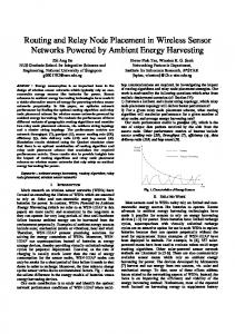
be the expected reduced number of relays per leaf by a star aggregation. Namely, to compute (α − β)/|L(i)| in Si : • α: Expected number of relays used when relays are placed on individual path to the BS without aggregation: sum of the star leaves expected relay count. • β : Expected number of relays used when relays are placed on the aggregation path: potential “denser” placement due to increased carried flow size. An aggregation on star S is beneficial when it is expected to reduce the relay number (δ(S) > 0). A precise description of δ computation is given in the following sections. Besides, an illustration of the star and δ is given in Fig. 1. Star Center

B. Evaluating Flow Aggregation’s Impact on Relay Number

Aggr. Relay

Basic Idea: Rather than greedily aggregating flows, we now evaluate whether aggregation is expected to reduce relay number under the bandwidth constraints. We conduct aggregation only when the aggregation is expected to reduce the relay number. We first give the following three definitions. Definition 5.1: The bandwidth-sufficient (communication) range to support k flows R(k) is the maximum range mapping to the (minimum) link bandwidth more than k · rs :

Aggr. Path

R(k) = ω(min{Bi }),

∀Bi ∈ B ∧ Bi ≥ k · rs

d(v, BS)  R(k)

-∑

-1)/|L(i)| Star S(i,L(i))

Non-Aggr. Relay Non-aggr. Path

Fig. 1. Star and the reduction index illustration. In δ(S), the underlined “-1” will be applied when the center is an extra relay we need to place: in placing the new layer node. It will not be applied when the center is an existing node: in aggregation in SN. Terms SN, SN RN, RN rs Be Ue R(k) R, B, ω

(9)

(10)

BS

BS

Note that Eq. 4 and Eq. 9 are not in a loop of computing range and rate. Eq. 4 is used to compute the expected bandwidth when an edge length is known. Eq. 9 is used to compute the expected edge length when its carried flow rate is known. Definition 5.2: We propose a metric called expected relay count (denoted by X ). X(v, k) predicts the relay number from v to BS when carrying k number of flows. In an obstacle free or sparse region, an approximate prediction is: X(v, k) =

δ(S)=(∑

Star Leaf

X(v, k) S(i, L(i)) δ(S) Ssn ,Sc ,S

Definitions Sending terminals (stream sending nodes). Steiner points (relay nodes). A uniform single flow sending rate at each SN. Achievable bandwidth based on distance of link e. e’s link utilization ratio: its carried flow rate divided by its bandwidth. Bandwidth-sufficient range for k number of flows. link bandwidth, communication range vectors and their mapping function from Table I. Expected relay count for v with k flows. A star with center i and leaves L(i). Leaves are the stream senders and the center is the stream receiver. (Relay) reduction index by a star S. The star vector in SN, the candidate star vector, the final compatible star vector for channel assignment.

TABLE II N OTATIONS .

C. Flow Aggregation in Sending Terminals SN

We can obtain a more accurate X(v, k) by using A∗ search to find the shortest obstacle-aware path and use its length to replace d(v, BS). Definition 5.3: We define a star (denoted by Si (i, Li )), or a star subgraph structure, to serve as the unit for flow aggregation. A star graph Si (i, Li ) is a complete bipartite graph K1,|Li | , or a tree with one center vertex i and the remaining vertices to be the leaves Li . We define that the star leaves are the stream senders and the star center is the stream receiver or the aggregation destination in the star. Star Si = (i, Li ) has |Li | number of leaves sending flow to center i, the aggregation point. Recall in the system model that TDMA scheduling eliminates the interference inside a star when leaves share a channel in transmission. We say two stars Si and Sj are compatible, iff they have distinct leaves and centers. The channel assignment scheme ensures no interference between stars. Definition 5.4: Given the star subgraphs and expected relay count, we propose the reduction index (denoted by δ(S)) to 423

Algorithm 1: Selecting leaves for a node i with maximum reduction index. 1 Input: Node i. Output: Leaves L(i) with reduction index δ(S(i, L(i)). 2 Form an i’s candidate leaf set by node j in current layer satisfying: (1)

farther from BS than i. (2) j is in the bandwidth-sufficient range of i. 3 Compute bandwidth Be for each link whose sender is in the candidate

leaf set and the receiver is i using Eq. 4. 4 Sort the candidate leaf set by distance to i in ascending order. 5 Add each node j ∈ i’s candidate leaf set to a bandwidth-allowed leaf

set BL(i) in order, until the sum of eji ’s link utilization ratio is greater than 1: Eq. 6 is violated. Each time when a new node is added: update reduction index by computing δ(S(i, BL(i))) as in Eq. 11. 6 i’s leaves Li is set as the BLi when it has the maximum reduction index.

Main Procedures • For each i ∈ SN not in 1-hop bandwidth-sufficient range of the BS, we form a star with center i, select its leaves and compute the reduction index δ by calling Alg. 1 to evaluate how much “benefit” we can obtain if using i as the

aggregation point to aggregate flows with different leaves. • Given all the possible star candidates, we have a loop of

selecting the star with the maximum reduction index and

SN RN

0

6

Bandwidth Allowed Leaf:

0 4

2

1

3

1

10

8 9 2 1

11

8 13

Current Layer

5

New Layer

BS

5

Obstacle

7

n

p

3

4

2Mbps

m

2

11 9

8Mbps

Leaf:

4

14 BS

SN RN

Obstacle

12

0

Candidate Leaf:

13

15

14

12

10

6

3

BS

(a) Relay placement example: flow aggregation (b) Leaf selection. (c) Select new layer position as star (d) Relay placement example: new layer relay in SN. center for aggregation. placement. Fig. 2. Illustration of relay node placement. (Uniform sending rate rs =3Mbps)

conduct aggregation until the reduction index of the star is negative. (With non-negative reduction index, aggregation never increases the number of relays). • The remaining nodes not from the selected stars, along with selected star centers, serve as the first layer node. They will be the input of Alg. 2 for the next step. All selected stars are inserted into a star vector in SN, or Ssn . • For each selected star with center i, we also transfer the flows from leaves to i and insert i to the routing path (relay path) for each leaf. In Alg 1, the reduction index δ(S(i, BLi )) is computed by: 

δ(S(i,BLi ))=

j∈BLi ∪i X(j,1)−X(i,|BLi |+1) |BLi |

(11)

Example of Leaf Selection: We illustrate reduction index computation with Fig. 2(b). For n1 , its candidate leaf set has 5 nodes: {n4 , n0 , n2 , n3 , n5 }, which are farther from the BS than n1 is. By greedily selecting nodes from the candidate set in ascending order to the BS, only three nodes are allowed before the capacity is full. Besides, we discover that δ reaches its maximum as 0.5 when only the first two leaves are used. Therefore, Ln1 ’s final leaf set has two nodes: n2 and n4 . Example of Aggregation: We illustrate the flow aggregation in SN in Fig. 2(a). Each node computes leaves and the reduction index δ . The node with maximum δ node n5 is chosen (δn5 = 2) to be aggregated with flow from n3 . With n5 and n3 eliminated, δ is recomputed for the rest nodes. Node n4 with maximum δn4 = 1 is selected as the destination for flows from n0 and n2 . The aggregation terminates as the rest of nodes n1 and n6 have maximum δ < 0.

by calling Alg. 3, we need to select a subset of stars with the maximum sum of star’s reduction index to form a final star vector S. A new layer relay will be placed in the center at each star in S. The stars in S must be compatible because they cannot share leaves or centers since a flow can only be aggregated to one destination under the bandwidth constraints. The problem is modeled as the NP-hard [17] maximum weighted set packing problem, which is defined as follows: Given a finite set and a list of subset, find the disjoint subsets with maximum sum of weight. In our problem, the finite set is the set of all the leaves of stars in Sc . Each star is a subset including its two leaves, and the star’s reduction index is the weight of the subset. Algorithm 2: New layer relay placement with flow aggregation. 1 Input: Current layer nodes. Output: New layer nodes; routing paths. 2 Form a candidate star vector Sc by a hypothetical placement of center

3

4

5 6

vertex k as destination for each pair of nodes in current layer. Call Alg. 3 times (k is the number of nodes in current layer). Use each node 2 pair to be Alg. 3’s input. Select a final star vector S with the maximum sum of reduction index from Sc : Iterate through Sc ’s powerset, filter out the incompatible subsets, and obtain the compatible subset with maximum of the sum of reduction index. Denote the resulting star vector S. New layer is set by the following two types of nodes: (1) Centers in S; (2) New nodes placed for non-aggregated flows for rest of the current layer nodes at bandwidth-sufficient range on the obstacle-aware paths to the BS by A* search. Flows and routing paths are updated similar to the procedure in Section V-C. Links with non-aggregated flows (a star with 1 center and 1 leaf) are also inserted into S. Besides, Ssn is appended to S.

Algorithm 3: Choose new layer node position for aggregation. 1 Input: Leaf positions m, n. Output: A candidate star S with center

D. New Layer Relay Placement with Flow Aggregation

position p and reduction index δ(S(p, L(p))) , where L(p) = {m, n}.

Overview: Given the first layer node as the current layer, the next layer nodes are placed to approach the BS. A new layer node is placed at the aggregation point to approach the BS if the flow aggregation is expected to reduce relays. Otherwise it is placed to be closer to the BS by its bandwidth-sufficient range, on the direct path from the current layer node to the BS. The major steps are in Alg. 2. Alg. 2 calls Alg. 3 to compute the next layer candidate relay positions. They are the potential aggregation destinations given the current node pairs. Select Compatible Stars with Maximum Sum of Reduction Index: In Alg. 2, given the candidate star vector Sc computed 424

2 Obtain range vectors Rm ⊆ R, Rn ⊆ R constrained by their bandwidth

requirement for the carried flow sizes. 3 Compute Bandwidth Be for links with length equal to each range

R ∈ Rm ∪ Rn by Eq. 4.

4 Test each pair < i, j > ∀i ∈ Rm , j ∈ Rn . When (1) total flows do not

exceed the shared bandwidth: Eq. 6 is not violated; and (2) valid overlapping area exists for range disks m and n: The closest position p to the BS in the overlapping area is saved as a candidate star center for this pair. 5 Final center p is the closest position to the BS among all candidate centers. Form S(p, Lp ) with leaves Lp = {m, n}. 6 Compute reduction index by Eq. 12. Add S(p, Lp ) to the candidate star vector Sc if δ(S(p, Lp )) > 0 (Not beneficial stars cannot be candidates: aggregation never increases the number of relays).

Due to the NP-hard nature of this problem, we compute the powerset to try all possible cases to obtain the optimal result when the input size is less than a threshold k: |Sc | ≤ k. (The powerset of a set is the set of all its subsets.) If |Sc | > k, we iteratively greedily select stars with the maximum reduction index to form S . In the simulation process, we set k = 12 and find that all our test cases have |Sc | < k and the results are computed efficiently. Choose the New Layer Node Position for Aggregation: In Alg 3, the reduction index δ(S(i, Li )) is computed by: 

δ(S(i,Li ))=

j∈Li X(j,|fj |)−1−X(i, |Li |



j∈Li |fj |)

(12)

where fj is the flow size carried by j . Note that the flexible position of the star center is the main difference compared to the aggregation in SN. The star center p is generally the closest position to the BS in the overlapping area of range disks of i, j . Note that it is possible all range combinations fail to provide bandwidth adequacy after aggregation. In addition, the formed star S is added to Sc only when beneficial: δ(S) > 0. Example of Choosing New Layer Node Position for Aggregation: Fig. 2(c) illustrates Alg. 3. Given a pair of current layer nodes m, n with fm =8Mbps, fn =2Mbps, the range sets Rm , Rn are known. Each pair of ranges for m, n are tested until we find the final position p. Note that p is not placed in m’s out-most disk because the maximum ranges m n = 115ft, Rmax = 191ft cannot be used together: for Rmax They exceed the bandwidth with sum of link utilization ratio  U = 8/10 + 2/5 = 1.2 > 1.0. Example of Aggregation: Fig. 2(d) illustrates placing new layer relays with flow aggregation. While n0 and n4 are too far apart to be aggregated, n7 and n8 are in range to aggregate each of its flow 3Mbps to n9 with 6Mbps. In addition, n1 ’s 6Mbps flow, including that from n2 , is aggregated with n3 ’s 3Mbps flow to n6 . Example of Relay Density Variance: Both Fig.2(a) 2(d) show relay density variation among paths with different flow sizes. In Fig. 2(d), more relays are placed on path from n6 than that from n9 to the BS. Likewise, relays are placed more sparsely for a single flow in path from n6 to the BS compared with other paths in Fig. 2(a). To sum up, flows are aggregated when they are expected to reduce relay number in placement. VI. C HANNEL A SSIGNMENT Algorithm 4: Channel assignment. 1 Input: Star vector S. Output: A channel assigned for each S ∈ S. 2 Construct star reduced graph (SRG) Gsrg (V, E) from S. 3 Construct link contention graph (LCG)

Glcg (V, E) ← Gsrg (L(V ), L(E)).

4 Compute channel distances for each e and update E in Glcg . 5 Vertices Vtmp ← V in Glcg . 6 while Vtmp is not empty do 7 8

i∗ ← argmaxi∈Vtmp j∈Vtmp ∧∃eij weighteij . Assign least unused channel ID to Si∗ . Remove i∗ from Vtmp .

Although relays are placed with selected flow aggregation and varying distances according to different flow sizes, bandwidth adequacy cannot be satisfied without proper channel assignment to eliminate the inter-star interference. We model

the channel assignment problem as the NP-hard bandwidth coloring problem [18] for a minimum total number of channels. Here, a channel represents the color. Bandwidth coloring problem generalizes the classical vertex coloring problem with the edge weight constraints on color distances of adjacent vertices. Such modeling enables us to tackle the problem of out-of-band (OOB) emission (or the adjacent channel interference with power leakage when radios are placed very close (less than 1m) [11]). To overcome this problem, we double the channel distance for the two radios at the same node, which is modeled by the doubled weight. A greedy algorithm is designed to choose the vertex with the maximum sum of adjacent edge weights (Detailed procedures are in Alg. 4). VII. P ERFORMANCE E VALUATION Summary • To evaluate the quality of the proposed method (for simplicity, we call our method HBSR), we compare HBSR to the widely used minimum spanning tree based approximation for relay placement. • To evaluate the benefit of considering heterogeneous range and rate, we compare HBSR to the uniform range and rate based relay placement. • In addition, we also apply HBSR to a coordinated mobility model where fewer relays can enable more robots to conduct search and thus increase the mobility efficiency. The mobility model is a multi-robot area exploration strategy with video aggregation [5]. We use a C++ simulation program with the Open and Garden environments as in Fig. 3(d), where obstacles are denoted by black cells. Both environments are represented by 150 × 150 grid cells with cell edge length of 6ft. Due to the exponential nature of HBSR, and the highly complex linear programming formulation for heterogeneous ranges and rates, we did not directly compare the results with the optimal or its lower bound. Instead we provided the upper bound of the approximation ratio to the optimal. We will carry out the direct comparison to optimal in future work. A. Comparing to Min. Spanning Tree based Relay Placement First, we compare the required relay number to a heterogeneous range and data placement scheme satisfying the bandwidth requirement. It is built upon a widely used approximation algorithm called the Steinerized Minimum Spanning Tree [19] (for simplicity we call this scheme S-MST) for relay placement. We choose S-MST for comparison because there is no existing algorithm exactly match our problem statement, but many solutions to the Steiner tree problem variants are based on the minimum spanning tree [1,3,6,19]. In S-MST, relay are added on the longer than R edges in MST to connect all terminals according to different flow sizes (R is the bandwidth-sufficient range). S-MST has a severe weakness of overflow that our scheme does not have: When all flows are aggregated to one SN and transmitted to BS via a single edge on the MST, flows may exceed the maximum link capacity (e.g. 25Mbps in Table I). Because of overflow and our interest to observe situations where bandwidth’s impact

425

25 20 15 10 5

25

30

HBSR S−MST Number of Relays

30

HBSR S−MST Number of Relays

Number of Relays

30

20 15 10 5

0 9 10 11 12 Num. of Sending Terminals (rs=2Mbps)

25

HBSR S−MST

20 15 10

0 5 6 7 8 Num. of Sending Terminals (rs=3Mbps)

5 0 3 4 5 6 Num. of Sending Terminals (rs=4Mbps)

(a) S-MST fails when |SN| >12. (b) S-MST fails when |SN| >8. (c) S-MST fails when |SN| >6. (d) Open and Garden environment. Fig. 3. (a)-(c): Compare relay number to bandwidth aware S-MST: Varied flow sending rate rs of 2-4Mbps. (d): Obstructive environments.

15

10

30 25

75

HBSR UR2−6Mbps UR2−12Mbps UR2−18Mbps

20 15 10

5

4

6 8 10 Number of Sending Terminals

12

5 360 450 540 630 720 Distance from SNs to BS (feet)

70 65 60

75 HBSR UR2−6Mbps UR2−12Mbps UR2−18Mbps

55 50 45 40 35 30 12

14 16 Total Number of Robots

18

Number of Iterations

20

Number of Relays

Number of Relays

HBSR UR2−6Mbps UR2−12Mbps UR2−18Mbps

Number of Iterations

35

25

70 65 60

HBSR UR2−6Mbps UR2−12Mbps UR2−18Mbps

55 50 45 40 35 30 12

14 16 Total Number of Robots

18

(a) Varying |SN|: 4-12. (b) Varied distance. |SN|=10. (c) Garden environment. (d) Open environment. Fig. 4. (a)-(b): Compare relay number to uniform range and rate relay placement (UR2 ): varied |SN| and distance to BS. (c)-(d): Compare exploration efficiency to UR2 based exploration by total number of iterations.

is non-trivial, we test on relay number with a fixed range of distance to the BS and use the highest four numbers of SN below overflow with varying sending rate rs from 2-4Mbps. All relay number tests in Section VII-A,VII-B are run 200 times to obtain the average in the Garden environment. We found that our algorithm is efficient and no instance runs more than one second. The 95% confidence interval is shown by the error bars. We use the polar coordinate (R, θ) to represent SN positions with the BS at (0, 0◦ ). R is random uniformly distributed in [R0 − β, R0 + β ]. When comparing with S-MST, we set R0 =480ft and β =240ft, and θ is uniformly distributed in [0◦ , 90◦ ]. Fig. 3 shows HBSR reduces the number of relays by 53.1%, 41.0%, and 38.6% on average. For the situations with the highest two SN numbers before overflow, the relay number reduction is more notable, which is 60.4% on average. B. Comparing to Uniform Range and Rate Relay Placement Second, we compare the number of relays to the uniform range and rate (UR2 ) scheme in [5] with two test sets: (1) Varying size of 4-12 SN with fixed range of distance to the BS (R0 =480ft and β =240ft). (2) Fixed size of 10 SN with varying ranges of distance to the BS (R0 ∈ {360, 480, 600, 720} (ft)); rs is set as 3Mbps hereafter. As shown in Fig. 4(a) 4(b), our scheme reduces the number of relays on average by 25.4%-39.0% and 25.5%-36.3% respectively in the two test sets compared to UR2 schemes with range corresponding to 618Mbps modulation data rates. (UR2 with rates above 18Mbps are not compared as they need notably more relays.) These results demonstrate the benefit of considering heterogeneous range and rate in relay placement because of its flexibility in adapting to different bandwidth and range requirements. C. Evaluating HBSR’s Impact on Mobility Efficiency We also apply HBSR to a coordinated multi-robot exploration strategy with video aggregation [5]. Relay placement is a critical component in its iterative mobility model. In each 426

round, a portion of the robots will be the relays and the remaining will be the “frontier” robots to explore the area. Less relays can enable more frontier robots to conduct search and thus increase the mobility efficiency. We compare the exploration-efficiency difference when using (1) HBSR vs. (2) UR2 to be the relay placement component. The S-MST is not evaluated here due to its overflow problem. We measured the number of iterations for exploration from a clustered start to 95% of explored area. Each robot has a sensing range of 48ft. Fig. 4(c) 4(d) demonstrate that the decrease in movement iteration number is on average 18.9%32.1% and 20.1-34.3% compared to UR2 6-18Mbps for the garden and open environments respectively given the total robot number of 12,14,16,18. Note that the improvement is also influenced by this specific exploration model in [5]. In future work, it is desirable to devise a heterogeneous mobile robot exploration model to fully exploit HBSR’s benefit. The figures also show that a single range and rate choice has the least number of movement iterations for a certain total robot number; however, exploration with this range and rate may not have the least iterations for other total robot numbers. This fact also demonstrates that a single transmission range based placement lacks the flexibility to adapt to different node densities and the total bandwidth demands. VIII. C ONCLUSION AND F UTURE W ORK Instead of aiming at prolonging the network time, we consider the relay placement and routing jointly to achieve bandwidth sufficiency for real-time multimedia aggregation. Heterogeneous link capacity and transmission range is considered because multimedia streams demand high bandwidth and affect the transmission range that supports the streams. We formulate the problem as a new variant of the Steiner tree problem called the heterogeneous bandwidth Steiner routing problem (HBSR). We show HBSR’s NP-hardness and the upper bound of our solution’s approximation ratio. Our solution

to HBSR places relay nodes iteratively and aggregates flows when the aggregation is predicted to reduce the number of relays, reducing relay number by an average of 44% compared to the widely used minimum spanning tree based algorithm. We also found that considering heterogeneous range and rate is beneficial in relay placement and significantly reduces the number of relays compared to the uniform range and rate placement. A single range and rate lack the flexibility to adapt to different stream demands of rates and ranges. Besides the applications in static sensor or camera networks, the proposed relay placement can also be applied in designing more efficient and QoS-aware mobility strategy in coordinated mobile robot networks. Such mobile robot network will be an ideal platform for tasks of remote sensing and control (e.g., the search and teleoperation tasks in 2011 Japan earthquake and nuclear crisis) where the video aggregation is essential. Future work may include: (1) real experiments with the video aggregation testbed, (2) improving the algorithm with a tighter approximation ratio or directly comparing to the optimal result, (3) considering CSMA/CA with more complex interference impact and the probability based range and rate, and (4) considering fault tolerance and survivability. R EFERENCES [1] S. Misra, S. D. Hong, G. Xue, and J. Tang, “Constrained relay node placement in wireless sensor networks: Formulation and approximations,” Networking, IEEE/ACM Transactions on, vol. 18, no. 2, 2010. [2] F. Wang, D. Wang, and J. Liu, “Traffic-aware relay node deployment for data collection in wireless sensor networks,” in IEEE SECON 2009. [3] X. Cheng, D. Du, L. Wang, and B. Xu, “Relay sensor placement in wireless sensor networks,” Wireless Networks, vol. 14, no. 3, 2008. [4] X. Han, X. Cao, E. Lloyd, and C.-C. Shen, “Fault-tolerant relay node placement in heterogeneous wireless sensor networks,” in IEEE INFOCOM 2007. [5] Y. Pei, M. Mutka, and N. Xi, “Coordinated multi-robot real-time exploration with connectivity and bandwidth awareness,” in ICRA 2010. [6] F. Wang and J. Liu, “Networked wireless sensor data collection: Issues, challenges, and approaches,” Comm. Surveys Tutorials, IEEE, 2010. [7] B. Lin, P.-H. Ho, L.-L. Xie, X. Shen, and J. Tapolcai, “Optimal relay station placement in broadband wireless access networks,” Mobile Computing, IEEE Trans. on, vol. 9, no. 2, feb. 2010. [8] “Key performance benefits of 802.11n,” www.cisco.com. [9] R. Draves, J. Padhye, and B. Zill, “Routing in multi-radio, multi-hop wireless mesh networks,” in MobiCom 2004. [10] P. Huang, C. Wang, L. Xiao, and H. Chen, “RC-MAC: A receiver-centric medium access control protocol for wireless sensor networks,” in IEEE IWQoS 2010. [11] S. Kakumanu and R. Sivakumar, “Glia: a practical solution for effective high datarate wifi-arrays,” in MobiCom 2009. [12] J. C. Chen, “Measured performance of 5-GHz 802.11a wireless LAN systems, 2001, available online, Atheros Inc.” [13] “FCC 15.407 as of august 8, 2008 - hallikainen.com, available online,” http://sujan.hallikainen.org/FCC/FccRules/2008/15/407/. [14] Y. Pei, M. Mutka, and N. Xi, “Connectivity and bandwidth aware real-time exploration in mobile robot networks,” in Wiley Wireless Communications and Mobile Computing, WCM (in press). [15] D. Halperin, W. Hu, A. Sheth, and D. Wetherall, “Predictable 802.11 packet delivery from wireless channel measurements,” in SIGCOMM 2010. [16] P. Barsocchi, S. Lenzi, S. Chessa, and G. Giunta, “Virtual calibration for rssi-based indoor localization with ieee 802.15.4,” in IEEE ICC 2009. [17] P. Crescenzi and V. Kann, “A compendium of NP optimization problems,” p. 52, 1998. [18] E. Malaguti and P. Toth, “A survey on vertex coloring problems,” in International Transactions in Operational Research, 2010. [19] D. Du and X. Hu, Steiner Tree Problems In Computer Communication Networks. World Scientific Publishing Co., 2008, pp. 177–193.

A PPENDIX Theorem 1. The HBSR problem is NP-hard. Proof: We prove the theory by contradiction. Suppose we have a polynomial solution to this problem, by relaxing the constraint by giving an infinite link capacity and a single transmission range, the problem becomes the Steiner minimum tree Problem with minimum number of Steiner points (SMT-MSP) [3], which will then be polynomially-solvable by our solution. This contradicts the fact that SMT-MSP is NP-hard [3], and this completes the proof. Theorem 2. Our solution to HBSR is extensible to deal with non-uniform flow sending rates rs from SN. Proof: In the current solution, the flow aggregation in SN assumes each flow sending rate is uniform, while the new layer node placement already assumes different flow sizes after possible aggregations in SN. The major changes to support non-uniform sending rates rs are as follows. (1) Change from the number of carried flows to the sum of all flow rates on a link in Eq. 11 and 12. (2) The expected relay count needs to be updated with a new bandwidth sufficient range in Eq. 9 mapping to the minimum link bandwidth  more than rs rather than k · rs . (3) The sorting in step 3 in Alg. 1 is now based on the ascending order of link utilization ratio rather than the distance to BS. These changes enable the reduction index computation with heterogeneous sending rates and this completes the proof. Upper Bound of Approximation Ratio: We derive the upper bound of the approximation ratio of our solution to HBSR. First we define some notations. R gives the transmission range corresponding to a single flow rate rs from each SN. Furthermore, Bm represents the maximum link bandwidth Bm = maxBi ∈B {Bi }, i.e., Bm = 25Mbps according to Table I. A maximum degree in a graph G is: Δ(G) = max{degG (v)|v ∈ V (G)}. We denote n, ns , nd , and nopt are the respective relay number obtained by: (1) algorithm for HBSR; (2) S-MST: the Steinerized minimum spanning tree [19] with a uniform range R not considering the flow constraint; (3) DT: direct tree, or the simple aggregation tree (star graph with center BS) where all flows from SN are directly relayed to BS without aggregation; and (4) Topt : An optimal Steiner tree with flow constraint and heterogeneous ranges that requires minimum number of relays. All four schemes except (2) satisfy our problem statement. Besides, we use MST to denote the minimum spanning tree for SN and BS. Note that DT and MST are two very simple tree structures easily obtained when given the input of SN and BS. We define κ = nd /ns =  e∈E(DT ) e/R/ e∈E(M ST ) e/R, where κ is the ratio of relays size for DT over that of MST with uniform range R. Thus, κ is relevant to SN and can be directly obtained from the input of HBSR. Theorem 3. The approximation ratio of our relay placement algorithm is no greater than κ · (1 + Bm /rs ). In an environment where obstacle distribution does not affect the triangular inequality, the ratio is no greater than κ · min{5, 1 + Bm /rs }. Proof: With an optimal tree Topt , we duplicate each edge and build an Eulerian tour such that every Steiner point appears at most Δ(Topt ) times in the tour while every terminal point appears exactly once. Removing one (or more) edge in the tour will give a spanning tree T  where Steiner points have degree at most two. Its Steiner point size n(T  ) is no more than Δ(Topt ) times in Topt . Because ns is from S-MST: a minimum spanning tree with relays on uniform non-shortened edges for single flows. Clearly, we have: ns ≤ n(T  ) ≤ Δ(Topt ) · nopt

(13)

With κ = nd /ns and the fact that flow aggregation guarantees n ≤ nd , we have: (14) n ≤ nd ≤ κ · Δ(Topt ) · nopt n/nopt ≤ κ · Δ(Topt ) (15) Lemma 1. Every Steiner tree that satisfies the flow constraint must have its maximum degree Δ(T ) ≤ 1 + Bm /rs . Proof: For a vertex, its incoming degree is the same as the number of incoming flows for aggregation, which is constrained by the maximum link bandwidth Bm . As we allow only one outgoing link, the total degree is at most Δ(T ) ≤ 1 + Bm /rs . Lemma 2. There exists a shortest optimal Steiner tree Topt whose maximum degree is less than or equal to five, i.e., Δ(Topt ) ≤ 5, in an obstacle-free area or obstructive area where triangular inequality holds [19]. From Lemma 1 and 2, Δ(Topt ) = min{5, 1 + Bm /rs } in obstacle free area or obstructive area where triangular inequality holds. Otherwise: Δ(Topt ) = 1 + Bm /rs . Replacing Δ(Topt ) concludes the proof.

427