Knowledge Discovery in Multiple Spatial Databases - Springer Link

Neural Comput & Applic (2002)10:339–350 Ownership and Copyright  2002 Springer-Verlag London Limited

Knowledge Discovery in Multiple Spatial Databases Aleksandar Lazarevic and Zoran Obradovic Center for Information Science and Technology, College of Science and Technology, Temple University, Philadelphia, PA, USA

In this paper, a new approach for centralised and distributed learning from spatial heterogeneous databases is proposed. The centralised algorithm consists of a spatial clustering followed by local regression aimed at learning relationships between driving attributes and the target variable inside each region identified through clustering. For distributed learning, similar regions in multiple databases are first discovered by applying a spatial clustering algorithm independently on all sites, and then identifying corresponding clusters on participating sites. Local regression models are built on identified clusters and transferred among the sites for combining the models responsible for identified regions. Extensive experiments on spatial data sets with missing and irrelevant attributes, and with different levels of noise, resulted in a higher prediction accuracy of both centralised and distributed methods, as compared to using global models. In addition, experiments performed indicate that both methods are computationally more efficient than the global approach, due to the smaller data sets used for learning. Furthermore, the accuracy of the distributed method was comparable to the centralised approach, thus providing a viable alternative to moving all data to a central location. Keywords: Distributed learning; Heterogeneous data sets; Local regression; Multiple spatial databases; Spatial clustering

Correspondence and offprint requests to: A. Lazarevic, Center for Information Science and Technology, Temple University, Room 303, Wachman Hall (038–24), 1805 N. Broad St., Philadelphia, PA 19122, USA.

1. Introduction Advances in spatial databases have allowed for the collection of huge amounts of data in various Geographic Information Systems (GIS) applications, ranging from remote sensing and satellite telemetry systems, to computer cartography and environmental planning. Many large-scale spatial data analysis problems involve an investigation of relationships among attributes in heterogeneous data sets, where rules identified among the observed attributes in certain regions do not apply elsewhere. Therefore, instead of applying global recommendation models across: entire spatial data sets, models are varied to better match site-specific needs, thus improving prediction capabilities [1]. An approach for analysing heterogeneous spatial databases in both centralised and distributed environments is proposed in this study. In the centralised approach, spatial regions having similar characteristics are first identified using a clustering algorithm. The local regression models are built on each of these spatial regions, describing the relationship between the spatial data characteristics and the target attribute, and then applied to the corresponding regions [2]. However, spatial data are often inherently distributed at multiple sites, and are difficult to aggregate into a single database for a variety of practical constraints, including dispersed data over many different geographic locations, security services and reasons of competition. In such a distributed environment, where data are dispersed, our proposed centralised approach of building local regressors [2] cannot be directly applied, since an efficient implementation of the data clustering step assumes the data are centralised to a single site. Therefore, a new approach for distributed learning based on

340

locally adapted models is also proposed. Given a number of distributed, spatially dispersed data sets, we first define more homogenous spatial regions in each data set using a distributed clustering algorithm. Distributed clustering involves applying a spatial clustering algorithm independently on all sites, and then identifying the corresponding clusters on participating sites. The next step is to build local regression models on identified clusters, to transfer models among the sites, and to combine the corresponding ones in order to improve the prediction accuracy on discovered clusters. The proposed methods, applied to three synthetic heterogeneous spatial data sets, indicate that both centralised and distributed methods are more accurate and more efficient than the global prediction method, and they are robust to a small amount of noise in the data. Furthermore, the distributed method was almost as accurate as when all data is localised at a central machine.

2. Related Work In contemporary data mining, there are very few algorithms available for clustering data naturally dispersed at multiple sites. The main purpose of existing distributed and parallel clustering algorithms is to speed up the clustering process by partitioning the entire data set into multiple processors. When the data is distributed over a very fast network with a limited bandwidth, and when the computer hosts are tightly coupled, several researchers have used a parallel approach to address this problem. This is particularly useful when the data sets are large and data analysis is computationally intensive. Recently, a parallel k-means clustering algorithm on distributed memory multiprocessors was proposed [3]. This algorithm is based on the message passing model of parallel computing, and it also exploits inherent data parallelism in the k-means algorithm. A simple, but effective, parallel strategy is to partition available n data points into P equal size blocks, and to assign the blocks to each of P processors. Each processor maintains a local copy of centroids for all k clusters, which have to be discovered. In a related study, Rasmussen and Willet [4] discussed parallel implementation of the single link (SLINK) clustering method on a Single Instructions Multiple Data (SIMD) array processor. Olson [5] described several parallel implementations of hierarchical clustering algorithms on an n-node CRCW PRAM, while Pfitzner et al. [6] presented a parallel clustering algorithm for finding halos

A. Lazarevic and Z. Obradovic

(luminous radiances) in N-body cosmology simulations. Unlike the algorithms described above, the parallel clustering algorithm PDBSCAN [7] is primarily designed for clustering spatial data. Based on the DBSCAN algorithm [8], PDBSCAN uses the ‘shared-nothing’ architecture, which has the advantage that it can be scaled up to hundreds of computers. Experimental results show that PDBSCAN scales up very well, and has excellent speed up and size-up behaviour. However, all of these parallel algorithms assume that the cost of communication between processors is negligible compared to the cost of actual computing and data processing, and that the time of utilising each processor is a critical factor of the cost and performance analysis. Nowadays, processing sites could be distributed over wide geographic areas, possibly across several countries or even continents. As a consequence, the cost of actual computation is now comparable to, and perhaps over-shadowed by, the cost of site-to-site communication and data transfer. The majority of the work for learning in a distributed environment, however, considers only two possibilities: moving all data into a centralised location for further processing, or leaving all data in place and producing local predictive models, which are later moved and combined via one of the standard methods [9]. With the emergence of new high-cost networks and huge amounts of collected data, the former approach may be too expensive and insecure, while the latter is too inaccurate. Recently, several distributed data mining systems, without data transfer among sites, have been proposed. The JAM system [10] is a distributed, scalable and portable agent-based data mining software package that provides a set of learning programs which compute models from data stored locally at multiple sites, and a set of methods for combining multiple computed models (meta-learning). A knowledge probing approach [11] addresses distributed data mining problems from homogeneous data sites, where the supervised learning process is organised into two learning phases. In the first phase, a set of base classifiers is learned in parallel from distributed data sets and in the second, the metalearning is applied to combine the base classifiers. Unlike the previous two systems, Collective Data Mining (CDM) [12] deals with data mining from distributed sites with a different set of relevant attributes (heterogeneous sites). CDM points out that any function can be expressed in a distributed fashion using a set of appropriate and orthonormal basis functions, thus leading to developing a general

Knowledge Discovery in Multiple Spatial Databases

framework for distributed data mining which guarantees the aggregation of local data models into a global model using minimal data communication. None of the distributed learning methods surveyed, however, provide analysis of data containing a mixture of distributions or spatial data analysis. Although there have been a number of spatial data mining research activities recently, most are primarily designed for learning in a centralised environment. GeoMiner [13] is such a system, representing a spatial extension of the relational data mining system DBMiner [14]. GeoMiner uses the Spatial and Nonspatial Data (SAND) architecture for modelling spatial databases, and includes the spatial data cube construction module, a spatial On-Line Analytical Processing (OLAP) module, and spatial data mining modules. Recently, a few proposed algorithms for clustering spatial data have been shown to be promising when dealing with spatial databases. In addition to the already mentioned DBSCAN algorithm, CLARANS [15] is based on randomised search, and is partially motivated by the k-medoid clustering algorithm, CLARA [16], which is very robust to outliers and handles very large data sets quite efficiently. Another example is the density-based clustering approach called Wave Cluster [17], that is based on wavelet transformation. The spatial data is considered as multidimensional signals on which the signal processing techniques (wavelet transforms) are applied in order to convert spatial data into the frequency domain.

3. Centralised Clustering-Regression Approach Given the training and test parts of a spatial data set, the first step in the proposed approach is to identify more homogeneous spatial regions in the training and test data. Partitioning spatial data into regions having similar attribute values is likely to result in regions of a similar target value. To eliminate irrelevant and highly correlated attributes, performance feedback feature selection [18] was used. The feature selection involved inter-class and probabilistic selection criteria using Euclidean and Mahalanobis distance, respectively [19]. In addition to sequential backward and forward search techniques applied with both criteria, the branch and bound search was also used with Mahalanobis distance. To test feature stability, feature selection was applied to different data subsets, and the most stable features were selected. In contrast to feature selection, where a decision

341

is target-based, variance-based dimensionality reduction through feature extraction is also considered. Here, linear Principal Components Analysis [19] and nonlinear dimensionality reduction using four-layer feedforward Neural Networks (NN) [20] were employed. The targets used to train these NNs were the input vectors themselves, so the network is attempting to map each input vector onto itself. We can view this NN as two successive functional mappings. The first mapping, defined by the first two layers, projects the original d-dimensional data into an r-dimensional sub-space (r ⬍ d), defined by the activations of the units in the second hidden layer with r neurons. Similarly, the last two layers of the NN define an inverse functional mapping from the r-dimensional sub-space back into the original d-dimensional space. Using features derived through feature selection and extraction procedures, the spatial clustering algorithm DBSCAN [8] was employed to partition the spatial data set into ‘similar’ regions. The DBSCAN algorithm relies on a density-based notion of clusters, and was designed to discover clusters of an arbitrary shape. The key idea of a densitybased cluster is that, for each point of a cluster, its Eps-neighbourhood for a given Eps ⬎ 0 has to contain at least a minimum number of points (MinPts) (i.e. the density in the Eps-neighbourhood of points has to exceed some threshold), since the typical density of points inside clusters is considerably higher than the outside of clusters. The clustering algorithm was applied to merged training and testing spatial data sets without using the target attribute value. These data sets need not be adjacent since the x and y coordinates were ignored in the clustering process. As a result of a spatial clustering, a number of partitions (clusters), generally spread in both training and test data sets (Fig. 1), were obtained. Assume that partitions Pi are split into the regions Ci for the training data set and regions Ti for the test data set. Finally, two-layer feedforward Neural Network (NN) regression models, with the Levenberg– Marquardt [21] learning algorithm, were trained on each spatial part Ci, and were applied to the corresponding parts Ti in the test spatial data set.

4. Distributed Clustering-Regression Approach Our distributed approach represents a combination of distributed clustering and locally adapted regression models. Following the basic idea of centralised clustering (Section 3), and given a number of spatial

342

A. Lazarevic and Z. Obradovic

4.1. Learning at a Single Site Although the proposed method can be applied to an: arbitrary number of spatial data sets, for simplicity, assume first that we predict on the data set D2 by using local models built on the set D1. Each of k clusters C1j, j ⫽ 1, . . . k, identified at D1 (k ⫽ 5 in Fig. 2) is used to construct a corresponding local regression model Mj. To apply models Mj to unseen data set D2, we need to match discovered clusters on D1 and D2. In the following subsections, two methods for matching clusters are investigated. Fig. 1. A spatial cluster P1, shown in (x, y) space, is split into a training cluster C1 and a corresponding test cluster T1.

dispersed data sets, the DBSCAN clustering algorithm is used to partition each spatial data set independently into ‘similar’ regions. As a result, a number of partitions (clusters) on each spatial data set are obtained. Assuming similar data distributions of the observed data sets, the number of clusters on each data set is usually the same (Fig. 2). If this is not the case, by choosing the appropriate clustering parameters (Eps and MinPts), the discovery of an identical number of clusters on each data set can be easily enforced. The next step is to match the clusters among the distributed sites, i.e. to determine which cluster from one data set is the most similar to which cluster in another spatial data set. This is followed by building local regression models on identified clusters at sites with known target attribute values. Finally, the learned models are transferred to the remaining sites, where they are integrated and applied to estimate unknown target values in the appropriate clusters.

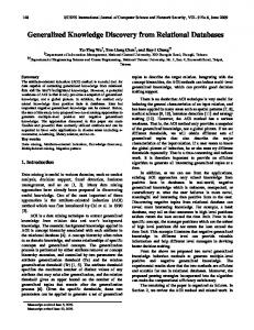
4.1.1. A Cluster Representation with a Convex Hull. To apply local models trained on subsets of D1 to an unseen data set D2, we construct a convex hull for each cluster on D1, and transfer all convex hulls to a site containing unseen data set D2 (Fig. 2). Using the convex hulls of the clusters from D1 (shown as H1,j in Fig. 2), we identify the correspondence between the clusters from two spatial data sets. This is determined by identifying the best matches between the clusters C1,j (from the set D1) and the clusters C2,j (from the set D2). For example, the convex hull H1,3 in Fig. 2 covers both the clusters C2,3 and C2,4, but it covers C2,4 in a much larger fraction than C2,3. Therefore, it can be concluded that the cluster C1,3 matones the cluster C2,4, and hence the local regression model M3 designed on cluster C1,3 is applied to cluster C2,4. There are also situations, however, where exact matching cannot be determined, since there are significant overlapping regions between the clusters from different data sets (e.g. the convex hull H1,1 covers both the clusters C2,2 and C2,3 in Fig. 2, so there in an overlapping region O1). To improve the prediction, averaging the local regression models built on neighbouring clusters is used on overlapping

Fig. 2. (a) Clusters in the feature space for the spatial data set D1; (b) clusters in the feature space for the spatial data set D2 and convex hulls (H1,i) from D1 (a) transferred to D2.

Knowledge Discovery in Multiple Spatial Databases

regions. For example, the prediction for the region O1 at Fig. 2 is made using the simple averaging of local prediction models learned on the clusters C1,1 and C1. In this way, we hope to achieve better prediction accuracy than local predictors built on entire clusters. An alternative method of representing the clusters, popular in the database community, is to construct a Minimal Bounding Rectangle (MBR) for each cluster, but this method results in large overlapping of neighbouring clusters. 4.1.2. A Cluster Representation with a Neural Network Classifier. In another method for determining the correspondence between regions (clusters) and constructed models, we treat each cluster as a separate group or class, and train a classifier on these groups. Here, a multilayer (2-layered) feedforward Neural Network (NN) classification model is used, with the number of output nodes equal to the number of classes (five as the number of clusters in the example from Fig. 2), where the predicted class is from the output with the largest response. The responses from the output nodes give us the possibility to compute probabilities of each data point belonging to a corresponding localised model. Therefore, this approach can be viewed as a mixture of experts with the NN classifier as a gating network [22], that can weight localised models according to computed probabilities. However, to simplify this approach in a distributed environment, we apply the NN classifier on an unseen spatial data set, associate predicted classes with the local models built on identified clusters, and then employ the models on determined classes. There is also a possibility of matching already discovered clusters on unseen spatial data set D2 with regions (classes) found by the NN classifier. For example, cluster C2,2 on data set D2 can contain several regions (classes) found by the NN classifier built on D1 (dashed lines in Fig. 3). For simplicity assume there are only two such identified classes

Fig. 3. Classes (regions) identified on data set D2 by a classification program built on data set D1.

343

(‘class1’ and ‘class5’ in Fig. 3) on cluster C2,2. These classes correspond respectively to clusters C1,1 and C1,5 from data set D1. By computing the percentage of ‘class1’ and ‘class5’ data points inside the cluster C2,2, we determine that a region (class) with greater ‘coverage percentage’ (‘class 1’ in Fig. 3) matches cluster C2,2 on data set D2. In addition, if the full correspondence between clusters and classes is not possible (the ‘coverage percentage’ by one region (class) is not significantly larger than the ‘coverage percentage’ by another class), we use simple average models built on both corresponding clusters at site D1. For example, when predicting on overlapping region O1 (Fig. 3) models built in clusters C1,1 and C1,5 are averaged. 4.2. Learning from Multiple Data Sites When data from multiple, physically distributed sites are available for modelling, the prediction can be further improved by integrating learned models from those sites. Without loss of generality, assume there are three dispersed data sites, where the prediction is made on the third data set (D3) using the local prediction models from the first two data sets D1 and D2. 4.2.1. Convex Hull Cluster Matching. To simplify the presentation, we discuss the algorithm only for the matching clusters C1,1, C2,2 and C3,2 from the data sets D1, D2 and D3, respectively (Fig. 4). The intersection of convex hulls H1,1, H2,2 and cluster C3,2 (region C in Fig. 4) represents the portion of the cluster C3,2, where clusters from all three fields are matching. Therefore, the prediction on this region is made by averaging the models built on the clusters C1,1 and C2,2, whose contours are represented in Fig. 4 by convex hulls H1,1 and H2,2, respectively. Making the predictions on the overlapping portions Ol, l ⫽ 1,2,3, is similar to learning at

Fig. 4. Transferring the convex hulls H1,1 and H2,2 from the sites D1 and D2 to a third site D3.

344

a single site. For example, the prediction on the overlapping portion O1 is made by averaging of the models learned on the clusters C1,1, C2,2 and C2,3, since the portion O1 corresponds to the part of the cluster determined by the convex hull H2,3, as well as belongs to the cluster C3,2 matched with the clusters given with the convex hulls H1,1 and H2,2. On the other hand, the prediction on the region O3 is performed combining the regressors built on the following clusters: C1,1, C1,4, C2,2 and C2,5. 4.2.2. A Cluster Representation with Multiple Classifiers. Using the same basic concept as in the twosite scenario, we independently employ classifiers to learn discovered clusters on each distributed site (sites D1 and D2) and to apply them to unseen data set D3. As a result, a number of class labels, equal to the number of data sites, are assigned to each data point on set D3. Each class label represents a cluster assignment for a particular data point predicted by a classifier from a specific data site. To make a prediction on such data points, a simple approach is to use non-weighted or weighted averaging of local models constructed on corresponding clusters from all data sites. Similar to the learning from a single site, an alternative method considers matching discovered clusters with regions (classes) identified by NN classifier, where averaging of local models is applied on potential overlapping regions.

5. Experimental Results Our experiments were performed on synthetic data set generated using our spatial data simulator [23] corresponding to five homogeneous data distributions, such that the distributions of generated data resembled the distributions of real life spatial data. The attributes (f4, f5) were simulated to form five clusters in their attribute space (f4, f5) using the feature agglomeration technique [23]. Instead of using one model for generating the target attribute on the entire data set, a different data generation process using different relevant attributes was applied for each cluster. Finally, the degree of relevance was also different for each cluster (distribution). The data sets had 6561 patterns with five relevant (f1–f5) and five irrelevant attributes (f6–f10). The histograms of a five attributes for all five distributions are shown in Fig. 5(a), while the target value level of the synthetic data set is shown in Fig. 5(b).

A. Lazarevic and Z. Obradovic

5.1. Modelling Centralised Heterogeneous Data A typical way to test the generalisation capabilities of regression models is to split the data into a training and a test set at random. However, for spatial domain such an approach is likely to result in overly-optimistic estimates of prediction error [2]. Therefore, the test field was spatially separated from the training field so that both fields were of approximately equal area, as shown in Fig. 1. We clustered the training and test patterns as an entire spatial data set using two relevant clustering attributes (f4, f5), and also using attributes obtained through the feature selection and feature extraction procedures. By setting the parameters of the DBSCAN algorithm, the clustering was applied so that the number of clusters discovered was always relatively small (5 to 10). For local regression models, we trained two-layer feedforward neural networks with 5, 10 and 15 hidden neurons. We chose the Levenberg–Marquardt [21] learning algorithm, and repeated the experiments starting from five random initialisations of network parameters. For each of these models, the prediction accuracy was measured using the coefficient of determination R2 ⫽ 1 ⫺ MSE/␴2, where ␴ is the standard deviation of the target attribute. The R2 value is a measure of the explained variability of the target variable, where 1 corresponds to a perfect prediction, and 0 to a mean predictor. In the most appropriate case, clustering is performed using only two relevant attributes (f4, f5) and regression models are built using all five relevant attributes (f1–f5). When clustering is performed using the attributes obtained through feature selection or feature extraction procedures, local regression models were built using identified attributes or all five relevant attributes (f1–f5), since our earlier experiments on these data sets showed that the influence of irrelevant attributes to modelling is insignificant. The prediction accuracies averaged over 15 experiments for different numbers of hidden neurons (5–15) are given in the Table 1. It is evident from Table 1 that the method of building local specific regression models (local regression approach) outperformed the global model trained on the entire training set and also the mixture of experts model (R2 ⫾ std ⫽ 0.83 ⫾ 0.03). Due to the overlapping cluster model assignment [23] and highly nonlinear models used in data generation, the R2 value achieved was not equal to 1. Results in Table 1 also suggest that the lack of relevant attributes either in spatial clustering or in the modelling process has a harmful effect on the global prediction

Knowledge Discovery in Multiple Spatial Databases

345

Fig. 5. (a) The histograms of all five relevant attributes for all five clusters; (b) the target value of the synthetic data set.

Table 1. R2 values for global and local regression approach when using different sets of attributes. Methods → Specified attributes ↓

All 5 attributes (f1–f5) 2 clustering attributes (f4, f5) 2 FS attributes (f1, f2) 3 FS attributes (f1, f2, f5) 4 FS attributes (f1, f2, f4, f5) 2 PCA attributes 3 PCA attributes

Global method with specified attributes (R2 ± std)

0.73 ⴞ 0.04 0.23 ⫾ 0.05 0.21 ⫾ 0.04 0.27 ⫾ 0.03 0.71 ⫾ 0.03 0.02 ⫾ 0.05 0.08 ⫾ 0.05

accuracy. When constructing global models with feature selection, the model is more accurate when using the more relevant attributes. Analogously, when building global models with attributes obtained through feature extraction, the prediction accuracy increases when the number of projections increases. When using attributes obtained through PCA for both spatial clustering and learning local regression models, it is evident that the proposed method suffers from the existence of irrelevant attributes, since the prediction accuracy was worse than applying a global model built with all attributes. When comparing the distributions obtained by applying spatial clustering with two relevant clustering attributes (f4, f5) (Fig. 2) to clusters identified using four most relevant attributes (Fig. 6(a)) or using three attributes obtained through PCA (Fig. 6(b)), it is apparent that the clusters discovered in the latter cases are disrupted by the existence of irrelevant clustering attributes. Clusters identified

Local regression approach where clustering is applied using specified attributes and modelling is performed with all attributes (R2 ± std)

with specified attributes (R2 ⫾ std)

0.78 ⫾ 0.03 0.87 ⴞ 0.02 0.76 ⫾ 0.03 0.75 ⫾ 0.03 0.80 ⴞ 0.04 0.71 ⫾ 0.05 0.72 ⫾ 0.04

0.78 ⫾ 0.03 0.37 ⫾ 0.03 0.22 ⫾ 0.02 0.25 ⫾ 0.03 0.72 ⫾ 0.03 0.18 ⫾ 0.01 0.31 ⫾ 0.03

shown in Fig. 6 have a fairly large overlap, and do not characterise the existing homogeneous distributions well. The influence of noise on prediction accuracy was tested using two noisy attributes responsible for clustering and five relevant but noisy attributes used for modelling. We experimented with different noise levels, and with different numbers and types of noisy attributes (attributes used for clustering and modelling, or for modelling only). The 5%, 10% and 15% of Gaussian additive noise in clustering and modelling attributes were considered for the total number of noisy attributes ranging from 1 to 5 (Fig. 7). Figure 7 shows that when a small amount of noise is present in the attributes (5%, 10%), even if some of them are clustering attributes, the method is fairly robust. For a small amount of noise, we can also observe a slight improvement in prediction accuracy due to the fact that small noise allows neural net-

346

A. Lazarevic and Z. Obradovic

Fig. 6. (a) Contours of the clusters identified using four most relevant attributes obtained through Feature selection; (b) contours of the clusters identified using three attributes obtained through PCA.

Fig. 7. The influence of different noise levels on the prediction accuracy. We added none, 1, 2 and 3 noisy modelling attributes to the 1 or 2 noisy clustering attribute, making it so that the total number of noisy attributes is ranging from 1 to 5. We have experimented with 5%, 10% and 15% of noise level per attribute. The prediction accuracies (R2 values) were averaged over 15 experiments.

works to avoid local minima [24], and to find a global minimum with greater probability. It can be observed that, in addition to neural networks, the DBSCAN algorithm is also robust to small noise. However, by increasing the noise level (15%), the prediction accuracy starts to decrease significantly. The case when one of two attributes responsible for clustering is missing can be treated as an extreme case of noisy attributes considered above. In each experiment we exchanged one of the relevant clustering attributes for the most relevant one obtained through the feature selection process, and performed spatial clustering. As a result, one large cluster (60– 70% of the entire spatial data set) and few relatively smaller clusters were identified. For comparison to the global approach, local regression models were still constructed using all relevant attributes, including missing clustering attributes. Therefore, we examined only the influence of the missing attributes on the process of finding more homogeneous regions (clusters). Although the clustering approach still outperformed

the global approach (Table 2), the difference was insignificant compared to the clustering approach with all attributes. This can be explained by the fact that clustering resulted in a poor quality of clusters (one large and few relatively small clusters). When clustering attributes (f4, f5) were available, but access to other relevant attributes was incomplete, the method of local regression models still outperformed the global prediction models, but the Table 2. Comparing the global- and clustering-based approaches when clusters are applied with incomplete information. Method Global approach

R2 ⫾ std 0.73 ⫾ 0.04

Clustering approach first clustering attribute 0.77 ⫾ 0.07 when missing (f4) second clustering 0.78 ⫾ 0.07 attribute (f5)

Knowledge Discovery in Multiple Spatial Databases

347

Table 3. The accuracy of prediction models when some relevant modeling attributes are not available. Regression Method

Data Set 1

Data Set 2

Data Set 4

Available attributes for modelling Global R2 ⫾ std Local R2 ⫾ std

f1, f2, f4, f5 0.48 ⫾ 0.10 0.63 ⫾ 0.03

f1, f3, f4, f5 0.48 ⫾ 0.05 0.64 ⫾ 0.05

f2, f3, f4, f5 f1, f4, f5 0.48 ⫾ 0.07 0.54 ⫾ 0.03 0.65 ⫾ 0.04 0.75 ⫾ 0.02

generalisation capabilities of both methods considerably dropped as compared to when all attributes were available (Table 3). 5.2. Modelling Distributed Heterogeneous Data To test our distributed algorithm, three spatial data sets were generated [23] analogous to the previous spatial data set. Each set represented a mixture of five homogeneous data distributions with five relevant attributes and 6561 patterns. We measured the prediction accuracy on an unseen spatial data set when local models were built using data from one or two data sets located at different sites. A spatial clustering algorithm was applied using two clustering attributes, while local regression models were constructed using all five relevant attributes. Table 4 shows the accuracies for distributed learning from a single site and from two sites when local models were averaged over 15 trainings of neural networks. The prediction accuracy for all proposed methods of local regression models significantly outperformed the global models (line 1), as well as the matching cluster method using MBRs (line 3). By combining the models on overlapping regions (lines 5, 7), the prediction capability was further improved, and

Data Set 5

Data Set 3 f1, f2, f3, f4, f5 0.75 ⫾ 0.12 0.91 ⫾ 0.06

significantly outperformed the mixture of experts model (line 2). This indicated that, indeed, confidence in the prediction of the overlapping parts could be increased by averaging appropriate local predictors. When an overlapping region represented 10% or more of an entire cluster size, the experiments showed that it is worthwhile to combine local regressors in order to improve the total prediction accuracy. When models from two dispersed synthetic data sets were combined to make predictions on the third spatial data set, the prediction accuracy was slightly improved over the models from a single site (Table 4). It is also important to observe that the proposed distributed methods, when applied to synthetic data, successfully approached the upper bound of a centralised model, where all spatial data sets were merged together at a single site. We also repeated the experiments with different noise levels in attributes, and with different numbers and types of noisy attributes (Fig. 8) in a distributed environment. Similar to the experiments with noise in the centralised scenario, Fig. 8 shows that this approach was robust to small noise, but when the noise level was increased (15%), the prediction capabilities started to decay substantially.

Table 4. The prediction accuracy on data set D3 using models built on data set D1 or data sets D1 and D2. R2 ⫾ std

Method

Combine models from

1 Global model 2 Mixture of experts models 3 Matching clusters using Minimal Bounding Rectangles Matching clusters 4 Simple using convex hulls 5 Averaging for overlapping regions Classification based 6 Simple cluster learning 7 Matching ‘classes’ to clusters ⫹ averaging for overlapping regions 8 Centralised clustering (upper bound)

a single site

two sites

0.75 ⴞ 0.02 0.84 ⫾ 0.03 0.78 ⫾ 0.03 0.87 ⫾ 0.02 0.90 ⴞ 0.02 0.87 ⫾ 0.02 0.90 ⴞ 0.03

0.77 ⴞ 0.02 0.86 ⫾ 0.02 0.86 ⫾ 0.02 0.89 ⫾ 0.02 0.92 ⴞ 0.01 0.90 ⫾ 0.02 0.92 ⴞ 0.02

0.90 ⫾ 0.02

0.92 ⫾ 0.01

348

A. Lazarevic and Z. Obradovic

Fig. 8. The influence of different noise levels on the prediction accuracy in distributed learning from a single site. None, 1, 2 and 3 noisy modelling attributes were used in addition to 1 or 2 noisy cluster-defining attributes, making it so that the total number of noisy at ributes ranged from 0 to 5. We have experimented with 5%, 10% and 15% of noise level. Matching clusters using convex hulls were used.

5.3. Time Complexity of the Proposed Methods Both centralised and distributed clustering approaches require less computational time for making a prediction than the method of building global models, since the local regressors are trained on smaller data sets than the global ones, and the time needed for clustering is negligible compared to the time needed for training global neural network models (Fig. 9(a)). However, to estimate the complete performance of the distributed approach, the extra processing time (for constructing convex hulls or classifiers used for cluster representation) and communication overhead must be taken into account. In the ‘matching clusters’ approach, the time complexity for computing a convex hull of n points is ␪(n log n). In classification-based cluster learning, however, the time required for training a neural network for classification of clusters depends upon the number of training examples and the number of

hidden neurons, but it also depends upon the learned data distribution, which is not always predictable. In general, this time is linear in the number of training examples, but it is not apparent whether some of the suggested approaches are computationally superior. In addition, for a fixed (small) number of iterations needed for training a neural network model, classification-based cluster learning can be computationally less expensive, but not sufficiently accurate. Therefore, to determine the computational time needed for computing convex hulls and for training neural network classifiers for different numbers of data points, we measured the actual run time averaged over 50 experiments. Experimental results show that the approach of computing convex hulls requires much less computational time than the method of building neural network classifier (Fig. 9(b)). Communication overhead in our distributed approach includes data and information transfer among distributed sites. For the ‘matching cluster’ approach, the amount of data transferred among the

Fig. 9. (a) 쐌쐌쐌쐌쐌: the computational time needed for the global and centralised clustering approaches on the spatial data sets with 6561 data examples; · · · · ·: time needed for training five local regression modes on five discovered clusters with 793, 884, 1008, 1775 and 2101 data examples: —: time needed for training Neural Networks (NN) depending on the training set size; – – –: clustering time depending on the data set size; (b) the computational time for computing convex hulls and NN classifiers.

Knowledge Discovery in Multiple Spatial Databases

data sites depends upon the shapes of the clusters discovered, and cannot be predicted in advance. However, in our experiments the number of points needed to represent a convex hull was small (10– 30 data points), and the total data transfer (including convex hulls for all identified clusters) was 5– 15 KB. For classification-based cluster learning, it is clear that the transferred information is only a neural network model whose size depends upon the number of hidden layers and the number of hidden neurons at each hidden layer, and in practice is relatively small. For example, our implementation of a two-layered feed-forward neural network with five input and five hidden nodes required about 27 KB. Therefore, the data amount needed to be transferred is relatively small in both approaches, but due to much less time being needed to construct convex hulls, it is clear that this approach has a better total computational performance than the classification-based method, while achieving the same or even slightly better total prediction accuracy.

6. Conclusions A new method for knowledge discovery in centralised and distributed spatial databases is proposed. It consists of a sequence of non-spatial and spatial clustering steps, followed by local regression. The new approach was successfully applied to three synthetic heterogenous spatial data sets. Experimental results indicate that both the centralised and distributed methods can result in better prediction compared to using a single global model. We observed no significant difference in the prediction accuracy achieved on the unseen spatial data sets, when comparing the proposed distributed clustering-regression to a centralised method with all data available at the single data site, and when the data distributions at distributed sites were similar. However, when the data distributions at multiple sites were not alike, it is possible that the distributed approach may not be as accurate as the centralised one, since it is more convenient for distributed environments with comparable data distributions. The communication overhead among the multiple data sites in the distributed approach is fairly, small in general. In all distributed methods, local regression models constructed on the clusters identified were migrated to the site where prediction is made. All this information, which needs to be transferred, contains insignificant amounts of data, since models do not require a lot of space for their description.

349

In practice, distributed data mining very often involves; security issues when, for a variety of competitive or legal reasons, data cannot be transferred among multiple sites. In such situations, the first method of matching clusters by moving convex hulls is not quite adequate, although a very small percentage (usually less than 1%) of the data needs to be transferred. Therefore, when distributed sites want to keep their data private, the classificationbased cluster learning approach is more appropriate, since only the constructed models are transferred among the sites, but it is also slightly less efficient. Furthermore, all the suggested algorithms are very robust to small amounts of noise in the input attributes. In addition, when some of the appropriate clustering attributes are missing, the prediction accuracy becomes only slightly better than the single global model. Therefore, when this is the case, some supervised techniques of finding homogeneous regions will be more suitable. Although the experiments performed provide evidence that the proposed approaches are suitable for distributed learning in spatial databases, further work is needed to optimise them in larger distributed systems, since the methods of combining models become more complex as the number of distributed sites increases. Acknowledgements. The authors are grateful to Xiaowei Xu for his valuable comments, and for providing the software for the DBSCAN clustering algorithm, to Dragoljub Pokrajac for providing generated data, to Celeste Brown for her useful comments, and to Jerald Feinstein for his constructive guidelines.

References 1. Hergert G, Pan W, Huggins D, Grove J, Peck T. Adequacy of current fertiliser recommendation for sitespecific management. In: Pierce F (ed), The State of Site-Specific Management for Agriculture, American Society for Agronomy, Crop Science Society of America, Soil Science Society of America, 1997; 283–300 2. Lazarevic A, Xu X, Fiez T, Obradovic Z. Clusteringregression-ordering steps for knowledge discovery in spatial databases. IEEE/INNS International Conference on Neural Networks, Washington, DC, 1999; 345, Session 8.1B 3. Dhillon IS, Modha DS. A data clustering algorithm or distributed memory multiprocessors. Workshop on Large-scale Parallel Knowledge Discovery in Databases, 1999 4. Rasmussen EM, Willet P. Efficiency of hierarchical agglomerative clustering using the ICL distributed array processor. J Documentation 1989; 45(1): 1–24 5. Olson CF. Parallel algorithms for hierarchical clustering. Parallel Computing 1995; 21(8): 1313–1325

350

6. Pfitzner DW, Salmon JK, Sterling T. Halo World: Tool: for parallel cluster finding in astrophysical Nbody simulations. Data Mining and Knowledge Discovery. 1998; 2(2): 419–438 7. Xu X, Jager J, Kriegel H-P. A fast parallel clustering algorithm for large spatial databases. Data Mining and Knowledge Discovery 1999; 3(3): 263–290 8. Sander J, Ester M, Kriegel H-P, Xu X. Densitybased clustering in spatial databases: the algorithm GDBSCAN and its applications. Data Mining and Knowledge Discovery 1998; 2(2): 169–194 9. Grossman R, Turinsky A. A framework for finding distributed data mining strategies that are intermediate between centralised strategies and in-place strategies. KDD Workshop on Distributed Data Mining, 2000 10. Stolfo SJ, Prodromidis AL, Tselepis S, Lee W, Fan D, Chan PK. JAM: Java Agents for Metalearning over distributed databases. Proceedings Third International Conference on Knowledge Discovery and Data Mining 1997; 74–81 11. Guo Y, Sutiwaraphun J. Probing knowledge in distribute data mining. Proceedings Third Pacific-Asia Conference in Knowledge Discovery and Data Mining, Beijing, China. Lecture Notes in Computer Science 1999; 1574: 443–452 12. Kargupta H, Park B, Hershberger D, Johnson E. Collective data mining: a new perspective toward distributed data mining. Advances in Distributed and parallel Knowledge Discovery, AAAI Press, 1999 13. Han J, Koperski K, Stefanovic N, GeoMiner: A system prototype for spatial data mining. Proceedings International Conference on Management of Data 1997; 553–556 14. Han J, Fu Y, Wang W, et al. DBMiner: A system

A. Lazarevic and Z. Obradovic

15.

16. 17.

18. 19. 20. 21. 22. 23. 24.

for mining knowledge in large relational databases. Proceedings Second International Conference on Knowledge Discovery and Data Mining 1996; 250– 255 Ng R, Han J. Efficient and effective clustering methods or spatial data mining. Proceedings of the 20th International Conference on Very Large Databases 1994; 144–155 Kaufman L, Rousseeuw PJ. Finding Groups in Data: An Introduction to Cluster Analysis. Wiley, 1990 Sheikholeslami G, Chatterjee S, Zhang A. WaveCluster: A multi-resolution clustering approach for very large spatial databases. Proceedings 24th International Conference on Very Large Databases, New York, NY 1998; 428–439 Liu L, Motoda H. Feature Selection for Knowledge Discovery and Data Mining. Kluwer Academic, Boston, 1998 Fukunaga K. Introduction to Statistical pattern recognition. Academic Press, San Diego, 1990 Bishop C. Neural Networks for Pattern Recognition. Oxford University Press, 1995 Hagan M, Menhaj MB. Training feedforward networks with the Marquardt algorithm. IEEE Trans Neural Networks 1994; 5: 989–993 Jordan MI, Jacobs RA. Hierarchical mixture of experts and the EM algorithm. Neural Computation 1994; 6(2): 181–214 Pokrajac D, Fiez T, Obradovic Z. A spatial data simulator for agriculture knowledge discovery applications. In review Holmstro¨ m L, Koistinen P. Using additive noise in back–propagation training. IEEE Trans Neural Networks 1992; 3(1): 24–38